Quantitative Analysis of Near-Infrared Spectroscopy Using the BEST-1DConvNet Model

Abstract

In the quest for enhanced precision in near-infrared spectroscopy (NIRS), in this study, the application of a novel BEST-1DConvNet model for quantitative analysis is investigated against conventional support vector machine (SVM) approaches with preprocessing such as multiplicative scatter correction (MSC) and standard normal variate (SNV). We assessed the performance of these methods on NIRS datasets of diesel, gasoline, and milk using a Fourier Transform Near-Infrared (FT-NIR) spectrometer having a wavelength range of 900–1700 nm for diesel and gasoline and 4000–10,000 nm for milk, ensuring comprehensive spectral capture. The BEST-1DConvNet’s effectiveness in chemometric predictions was quantitatively gauged by improvements in the coefficient of determination (R²) and reductions in the root mean square error (RMSE). The BEST-1DConvNet model achieved significant performance enhancements compared to the MSC + SNV + 1D + SVM model. Notably, the R² value for diesel increased by approximately 48.85% despite a marginal RMSE decrease of 0.92%. R² increased by 11.30% with a 3.32% RMSE reduction for gasoline, and it increased by 8.71%, accompanied by a 3.51% RMSE decrease for milk. In conclusion, the BEST-1DConvNet model demonstrates superior predictive accuracy and reliability in NIRS data analysis, marking a substantial leap forward in spectral analysis technology. This advancement could potentially streamline their integration into various industrial applications and highlight the role of convolutional neural networks in future chemometric methodologies.

1. Introduction

Advancements in chemometrics and instrumental measurement techniques have increasingly highlighted the application of near-infrared (NIR) spectroscopy analysis in scientific research and industrial applications because of its nondestructive, rapid, and precise nature. Its widespread application spans various sectors, including food science [1], environmental chemistry [2], daily chemical industry [3], traditional Chinese medicine [4], polymer materials [5], petroleum, and biochemistry [6].

The primary objective of NIR spectroscopic analysis is to establish quantitative analytical models that describe the relationship between NIR spectra and target components [7]. NIR spectroscopy (NIRS)—a nondestructive, swift, and accurate analytical technique—has made significant strides in recent decades, presenting a broad spectrum of future applications.

Traditional NIR spectroscopy analysis methods include principal component analysis (PCA), principal component regression (PCR), partial least squares (PLS), partial least squares regression (PLSR), and support vector machine regression (SVR). PCA, introduced in the 1930s, is a traditional spectral preprocessing method that transforms basic vectors to reduce data dimensionality. Aguiar et al. [8] effectively differentiated soil samples from various regions of Brazil using PCA and demonstrated the value of NIRS in rapid soil analysis. However, PCA is limited in its ability to directly consider the relationship between independent and dependent variables. In the 1960s, Herman Wold introduced PCR, which transforms the original independent variables into a new set of principal components for model construction, effectively addressing the shortcomings of traditional PCA. Stacey et al. [9] employed PCR and Fourier-transform infrared spectroscopy to measure the properties of respirable quartz, kaolinite, and coal in various mineral samples from different countries. Nonetheless, PCR considers only the variance of the explanatory variables without factoring in their relationships with the response variables.

In the 1970s, the introduction of PLS shifted the focus to not only the relationships between predictive variables but also their correlation with response variables. Wang et al. [10] combined three distinct PLS algorithms with NIRS for rapid quantification of polyphenols in dark tea. However, in practical applications, PLS is limited to linear relationships, potentially failing to capture the complex nonlinear relationships present in the data. The 1990s saw the emergence of support vector machine (SVM)—a method extensively used in NIRS estimations [11]—to address the inability of PLS to conduct nonlinear regression analyses. By employing kernel tricks to map data to a higher-dimensional space, SVM can linearly separate nonlinear problems, thereby managing complex nonlinear relationships that are challenging for PLS. Ding et al. [11] proposed a machine learning approach combining NIRS and comprehensive learning particle swarm optimization to enhance tea-quality grade classification, demonstrating the effectiveness of the proposed algorithm in boosting SVM prediction accuracy. However, the sensitivity of SVMs to hyperparameter selection necessitates cross-validation and entails high computational complexity.

Recently, artificial neural networks, particularly convolutional neural networks (CNNs), have been extensively applied across various domains. Their advantage lies in eliminating the need for a manual network structure or kernel function design and avoiding the computational intensity of cross-validation. Given the complexity and structural characteristics of one-dimensional spectral data, the CNN approach is suitable for NIRS. Jernelv et al. [12] investigated CNN’s performance of a CNN in spectral data classification and regression analysis and compared it with other chemometric methods such as SVM and PLSR. Their findings revealed CNN’s superiority of CNNs over traditional methods in unprocessed classification tasks. However, both CNN and traditional methods benefit from appropriate preprocessing and feature selection. Wang et al. [13] demonstrated the application of deep convolutional neural networks in NIRS data analysis, effectively distinguishing different tobacco cultivation regions. This research not only confirmed CNN’s robust capability in extracting complex spectral features but also highlighted its crucial role in big data mining and analysis. However, these successful applications are underpinned by a key challenge: the performance of a CNN relies heavily on the setting of its parameters, particularly the configuration of the network layers. In practical applications, optimizing these parameters, especially the network depth, to enhance learning efficiency and analysis accuracy remains an unresolved issue. Moreover, CNN models are prone to overfitting, especially with limited sample sizes. Deep networks also require significant computational resources, including high-performance GPUs and substantial memory, which may limit their application in resource-constrained environments. As “black box” models, the internal decision-making processes of CNNs are often difficult to interpret, which could be a drawback in applications requiring model transparency. Additionally, CNN models may need to be adjusted and trained for different datasets, reducing their generality and flexibility.

In the realm of CNN performance optimization, parameter setting, especially the network layer configuration, is of paramount importance. These parameters, including the number of layers, number of neurons per layer, choice of activation functions, learning rate, and batch size, profoundly influence learning methods and network efficiency [14]. Different parameter configurations can lead to significant variations in learning effectiveness and efficiency, thereby affecting the final analysis results. Manual adjustment of these parameters is not only time-consuming but also prone to suboptimal network performance. In this context, Mishra et al. [15] explored the utilization of deep learning models to improve traditional PLSR methods by employing Bayesian hyperparameter tuning for some parameter adjustments. Additionally, Benmouna et al. [16] focused on using CNNs to estimate the ripeness of Fuji apples and compared them with three alternative methods: artificial neural networks (ANN), SVMs, and k-nearest neighbors (KNN), underscoring the significance of parameter adjustment in CNNs and their superior performance compared to other methods. This raises a critical question: in the absence of sufficient automation tools, how can one effectively optimize CNN parameter configurations, particularly network layers and convolutional neuron numbers, to enhance the network learning efficiency and accuracy of the analysis results?

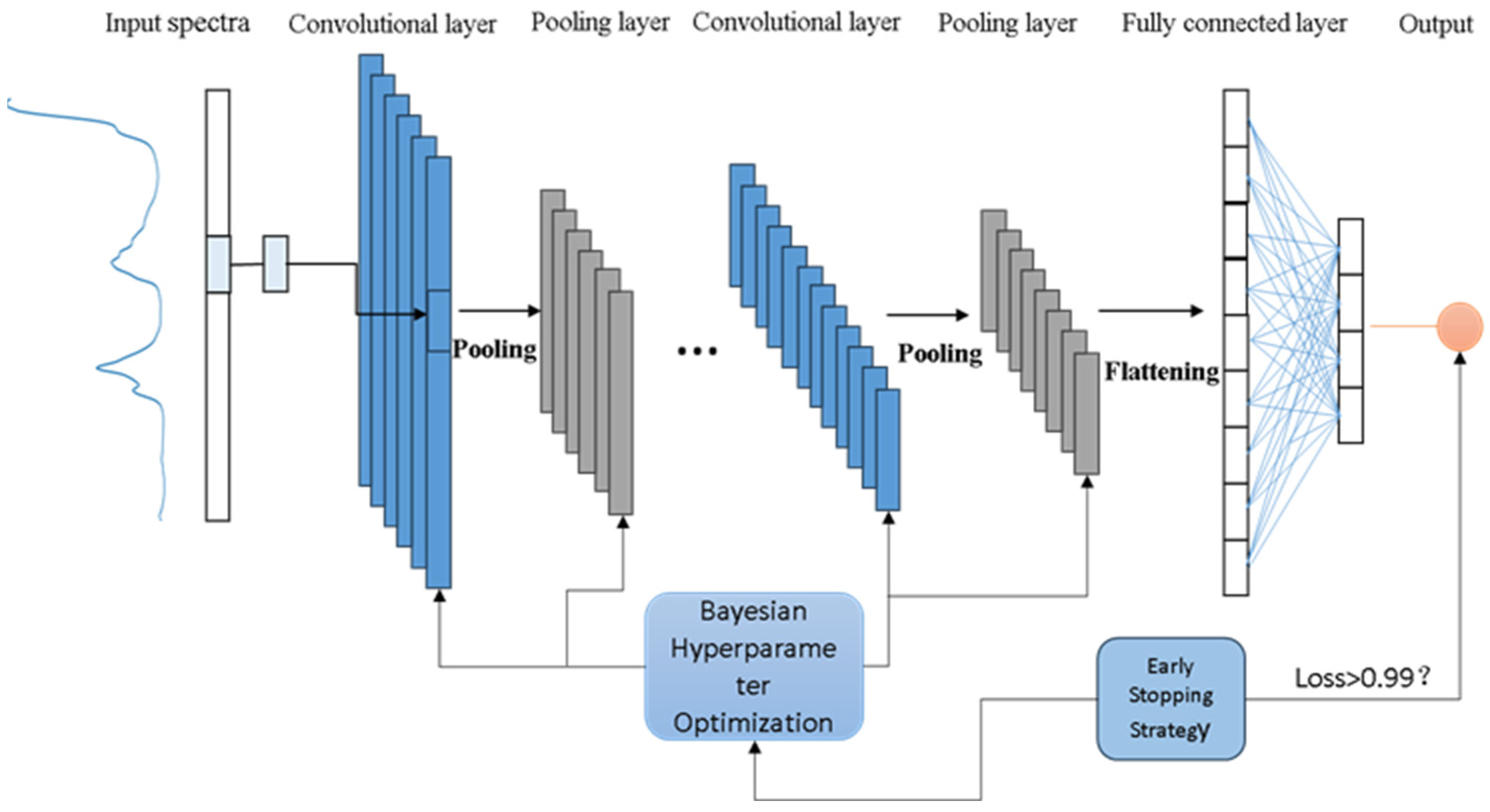
The core contribution of this study lies in the novel integration of Bayesian network hyperparameter optimization with early stopping strategies applied to one-dimensional CNNs, addressing the current parameter adjustment challenges. This innovative approach to neural network architecture searches not only maintains model generalizability but also automatically identifies the optimal model structure combinations. This method demonstrates significant advantages in processing complex spectral data to improve prediction accuracy and reliability. Moreover, it substantially reduces the need for manual parameter adjustments, thereby enhancing the efficiency of model development. Notably, this method exhibits exceptional generalizability across different datasets, eliminating the need to construct separate models for each data type. Using only the input data, the system can automatically determine the optimal parameter configuration, thereby achieving efficient and accurate predictions of the analysis results. This innovation not only optimizes the model performance but also showcases its unique value in practical applications, particularly in the precise analysis and prediction of complex data.

2. Materials and Methods

2.1. Data Set Sources

2.1.1. Diesel Fuel Dataset

The diesel fuel dataset provided by Eigenvector Research Inc. (https://www.eigenvector.com/). comprises public data from 112 different regional diesel samples. The samples were scanned using a Fourier transform near-infrared (FT-NIR) spectrometer (Provided by the United States Army Southwest Research Institute). The scanning range spanned from 900–1700 nm with a 2 nm interval, resulting in spectral curves with 401 wavelength points per sample. For more details, please refer to

Table 1. Detailed information on the three public datasets used in the experiment.

Dataset Name	Number of Samples	Wavelength Range (nm)	Interval (nm)
Diesel	112	900–1700	2
Gasoline	60	900–1700	2
Milk	67	4000–10,000	4

. The cetane number of each diesel sample was analyzed using chemometric methods. The infrared spectrum of the diesel fuel samples is shown in Figure 1A.

2.1.2. Gasoline Data Set

The public dataset for gasoline, sourced from the UCI Machine Learning Database of the University of California, Irvine, was obtained through scans using an FT-NIR spectrometer. Similar to the diesel dataset, the scanning range was 900–1700 nm at 2 nm intervals, yielding spectral curves with 401 wavelength points for each sample. For more details, please refer to Table 1. The infrared spectrum of the gasoline samples is shown in Figure 1B.

2.1.3. Milk Data Set

The milk sample data, referenced from the literature [17], were acquired using an Antaris II FT-NIR spectrometer (Thermo Fisher Scientific, Waltham, MA, USA) in transmission mode. The dataset comprised 67 milk samples, procured directly from a local marketplace in Changsha, China, each scanned 32 times, and the average values were recorded. The scanning interval was set at 4 nm, covering a wavenumber range of 4000–10,000 nm, resulting in 1557 spectral points. For more details, please refer to Table 1. Chemical methods were used to measure the protein content in each milk sample. The infrared spectrum of the milk samples is shown in Figure 1C.

2.2. Near-Infrared Spectroscopy (NIRS) Preprocessing

Given the high sensitivity of NIRS data to external environmental factors, preprocessing is an essential component of spectral signal analysis. Preprocessing is widely employed to eliminate or reduce unwanted variations in raw spectral data, such as noise bands, light contamination, and scattering effects [18]. In this study, three preprocessing methods were utilized: multiplicative scatter correction (MSC) to address the scattering effects in the spectra, standard normal variate (SNV) for drift issues, and first difference (1D) for baseline drift [19]. In addition to each of these methods, a combination (MSC + SNV + 1D) method was employed, and their respective impact on enhancing the model performance was ascertained. The preprocessing results for the three public datasets are shown in Figure 2. Figure 2A–D display the spectra of diesel after four different preprocessing methods, Figure 2E–H illustrate the spectra of milk, and 2I–L shows the spectra of petroleum, each processed using the four methods.

2.3. Overview of Spectral Analysis Using the BEST-1DConvNet Model

This section is divided into several subsections that provide a concise and precise description of the experimental results, their interpretation, and the experimental conclusions.

2.3.1. The 1D-ConvNet Model

CNNs are deep learning models that are structurally analogous to the human visual system and function as feedforward neural networks similar to VggNet, DenseNet, and AlexNet [20]. As depicted in Figure 3, the core component of a CNN is the convolutional layer, complemented by the activation function, pooling, and fully connected layers. The convolutional layer performs convolution operations on the input data using sliding windows (convolution kernels), as shown in Figure 3, to extract feature information [21]. The activation function layers facilitate nonlinear mapping, and the pooling layers generally reduce the dimensionality of feature vectors in the convolutional layers. To prevent overfitting, dropout layers were added, followed by fully connected layers that established a map between the extracted abstract features and the output target. For image data, convolution kernels are two-dimensional matrices; however, for time-series data, these kernels must be conceptualized as one-dimensional, leading to the development of one-dimensional convolutional neural networks (1D-CNNs).

The 1D-CNNs extend the convolution operation from a two-dimensional to a one-dimensional space, thereby enhancing the analysis of time-series data [22]. A 1D-CNN utilizes a convolution kernel that slides over an input sequence to extract the local features. Compared with traditional Recurrent Neural Networks (RNNs), 1D-CNNs offer the advantage of parallel computation, enabling more efficient processing of large-scale time-series data. Moreover, 1D-CNNs can construct deeper models by stacking multiple convolutional and pooling layers, thereby enhancing feature extraction capabilities.

In this study, the original one-dimensional infrared spectra were treated as a special set of two-dimensional images containing only one row or column. We then designed one-dimensional convolution kernels to match the one-dimensional infrared spectra. The convolution operation pattern between the original NIR spectra and the convolution kernels, as shown in Figure 4, reveals how the relationship between the stride and kernel size affects the convolution results [23]. If the stride is smaller than the convolution kernel (Figure 4A), overlapping regions occur across the entire range of the near-infrared spectrum. If the stride is equal to the convolution kernel (Figure 4B), the entire NIR spectral range is divided into several intervals, similar to the interval partial least squares (iPLS) method [24]. On the contrary, if the stride is larger than the convolution kernel (Figure 4C), some useful information may be lost [25]. Thus, we aim to avoid this scenario. Moreover, as different target components have different absorptions at each wavelength, the absorption information was accurately captured using multiple convolution kernels in the 1D-CNN model. In summary, the convolution kernels can not only extract abstract features of the NIR spectra but also select the most characteristic wavelengths.

2.3.2. Bayesian Hyperparameter Optimization and Early Stopping Strategy

Bayesian hyperparameter optimization plays a crucial role in the 1D-CNN model designed in this study. In particular, for the 1D-CNN parameter selection, this method shows that the network performance heavily depends on the hyperparameter configuration, such as the number of convolutional layers, kernel size, stride, pooling strategies, and neuron activation functions. Bayesian optimization outperforms the traditional grid and random search methods by intelligently navigating the hyperparameter space, considering potential interactions between parameters, and identifying optimal parameter combinations with fewer iterations.

Bayesian hyperparameter optimization constructs a probabilistic model for hyperparameters, leveraging Gaussian processes (GP) to predict the distribution of the model performance for given specific hyperparameter combinations [26]. For 1D-CNNs, this approach involves choosing new hyperparameter combinations in each iteration to maximize the acquisition function, such as the expected improvement (EI). This is significant for the 1D-CNNs used in sequential data processing, where the hyperparameters directly influence the ability of the model to capture temporal dependencies. Therefore, the EI function is defined as follows:

$$EI\left(x\right)=E\left[\max \right(0,{\mathrm{y}}_{\max }-\mathrm{f}\left(x\right)\left)\right]$$

(1)

where x denotes the hyperparameter combination; ymax is the highest target function value observed thus far; and f(x) represents the predicted mean of the GP model. This strategy aims not only to enhance the model performance but also to reduce computational resource consumption, which is crucial for large-scale data processing.

The early stopping strategy monitors the model performance on the validation set by intruding on a patience parameter p to prevent overfitting and premature training termination [27]. The early stopping condition is as follows:

$$\begin{array}{l}f min(RMS{E}_{val} )<RMS{E}_{val} [t-p] \\ for t>p,\\ then stop\end{array}$$

Under this condition, RMSEvalt−p signifies the root-mean-square error of the validation set at time t−p. By integrating Bayesian optimization with early stopping, the 1D-CNN network structure is designed to not only efficiently explore the hyperparameter space but also ensure that its training process is accurate and robust. This enhances the model’s ability to generalize new data, thereby improving the overall reliability and predictive accuracy.

2.3.3. BEST-1DConvNet Model

Bayesian hyperparameter optimization plays a crucial role in the 1D-CNN model designed in this study. In particular, for 1D-CNN parameter selection, this method shows that the network performance heavily depends on the hyperparameter configuration, such as the number of convolutional layers, kernel size, stride, pooling strategies, and neuron activation functions. To enhance efficiency and reduce practical limitations in the modeling process, a framework named BEST-1DConvNet was developed, employing Bayesian optimization techniques to automate and optimize the design of the CNNs.

In the BEST-1DConvNet framework, an NIRS dataset was loaded and preprocessed (including normalization) to ensure data compatibility with the convolutional network. The dataset was then split into training and testing sets by randomizing the data indices to ensure data representativeness and model generalizability. The framework further defines a ConvNet class, which is a custom 1D-CNN dynamically adjusted based on data characteristics and Bayesian optimization outcomes. This network is thus capable of adapting key parameters, such as the number of convolutional layers, filter size, and stride, thereby ensuring effective adaptation to varying data features. Using the skorch library, the PyTorch models were converted into estimators compatible with scikit-learn. This enables Bayesian optimization using BayesSearchCV to search for the best hyperparameter combinations. Additionally, a custom dataset-splitting function and split dataset provide training and validation sets during training. Early stopping strategies were applied to prevent overfitting and model performance was monitored by tracking training and validation losses. After identifying the optimal hyperparameter combination, the best model was constructed, and its network architecture was detailed for further analysis and optimization.

Finally, the performance of the model was evaluated on the test set by calculating the root mean square error (RMSE) and coefficient of determination (R²) values to quantify the predictive accuracy and reliability of the model. Furthermore, training and validation loss curves over time and scatter plots of the predicted versus actual values were generated to further visualize the model’s performance. The design process for the BEST-1DConvNet model is illustrated in Figure 5.

2.4. Evaluate the Metrics

RMSE and coefficient of determination (R²) were selected as the primary metrics for the model evaluation. These measures are instrumental in assessing the accuracy and reliability of predictive models. RMSE quantifies the deviation between the predicted and actual values by calculating the mean of the squares of these deviations and then extracting the square root. On the contrary, R² represents the squared correlation between the actual and predicted outputs, thereby reflecting the model’s reliability. The accuracy of the model can be assessed by calculating RMSE between the predicted and actual values, aiding in model selection and parameter optimization. The computation of RMSE is straightforward. It involves squaring the differences between each sample’s predicted and actual values, summing these squares, dividing by the number of samples to obtain the mean square error (MSE), and finally taking the square root of the MSE to arrive at the RMSE [28].

$$RMSE=\sqrt{\frac{1}{n}{\displaystyle \sum _{i=1}^n{({\widehat{y}}_i-y_i)}^2}}$$

(2)

R² (R-squared), also known as the coefficient of determination, is a statistical measure commonly employed to evaluate the fit of a regression model [29]. It quantifies the degree of similarity or explanatory power between the actual observed values and those predicted by the model. The formula for calculating R² is as follows:

$$R²=1-\frac{{\displaystyle \sum _{i=1}^n{(y_i-{\widehat{y}}_i)}^2}}{{\displaystyle \sum _{i=1}^n{(y_i-{\overline{y}}_i)}^2}}$$

(3)

Here, y represents the mean of the actual test samples, and $y_i$ and $\overline{y}$ denote the actual and predicted target output values for the ith sample, respectively. Variable n corresponds to the number of test samples. Generally, the closer the R² value is to 1, the closer the RMSE value approaches 0, indicating a superior overall performance of the model.

3. Results

3.1. Dataset Split

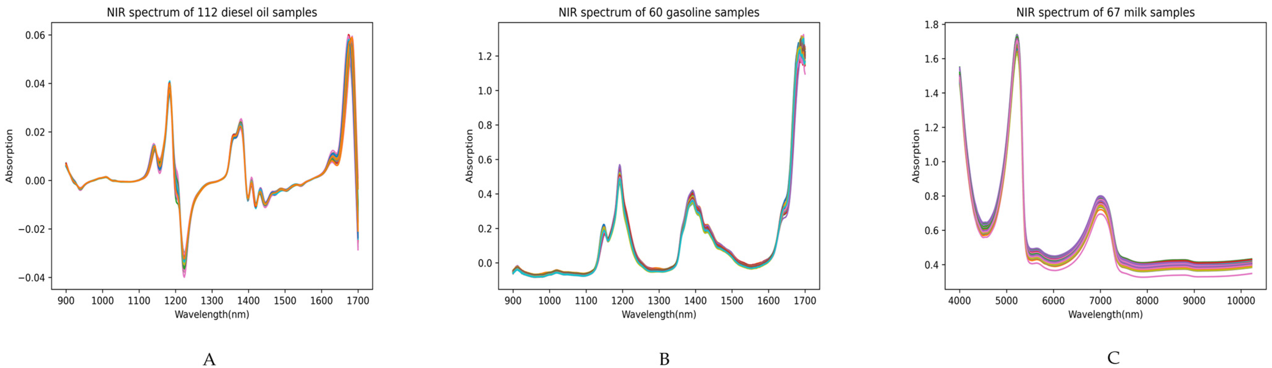
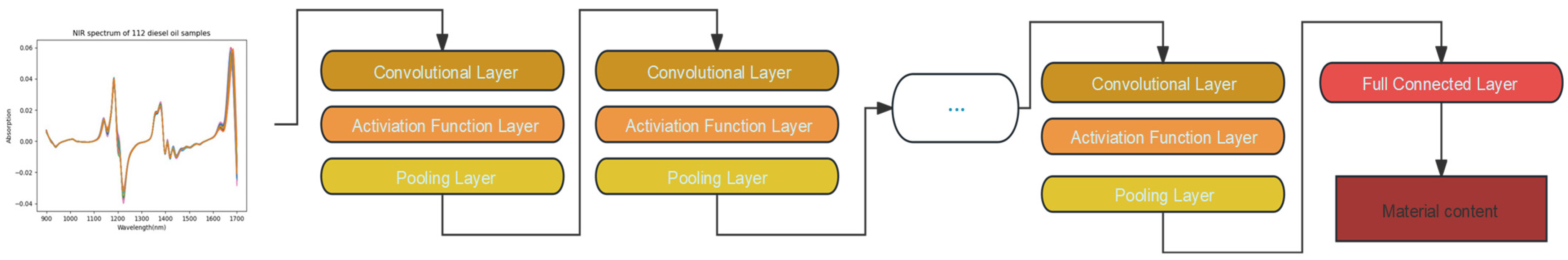
In this study, a 1D-CNN model is constructed using raw NIRS data. The dataset included 60 gasoline, 112 diesel, and 67 milk samples. These samples were divided into training and prediction sets in a 7:3 ratio. Specifically, for gasoline and diesel samples of varying concentrations, 70% were randomly selected for training the 1D-CNN model, whereas the remaining 30% were utilized for external prediction to evaluate the performance of the developed 1D-CNN model.

3.2. Training Results of SVM Modeling with Different Preprocessing Methods

A traditional machine learning technique, SVM, was employed for modeling. This approach was used to compare the post-preprocessing of the SVM and BEST-1D-CNN models. The SVM model utilizes the radial basis function as its kernel, with gamma set to ‘auto’ and the penalty parameter (C) set to 10. The performance metrics of the SVM model with and without preprocessing are listed in

Table 2. Evaluation of support vector machine network prediction.

Determination Parameters	Entire Sample Range	Model	R2	RMSE
CN-16	40.3~61.3	SVM	0.603334	2.403079
		MSC + SVM	0.632432	1.976964
		SNV + SVM	0.532454	2.562515
		1D+ SVM	0.609381	2.248109
		MSC + SNV + 1D + SVM	0.651380	1.839059
Octane Rating	83.4~89.6	SVM	0.778634	0.767548
		MSC + SVM	0.847493	0.651657
		SNV + SVM	0.613490	0.808224
		1D + SVM	0.799453	0.641156
		MSC + SNV + 1D + SVM	0.875780	0.512449
Protein	0.82869~3.47940318	SVM	0.773031	0.747649
		MSC + SVM	0.853190	0.411117
		SNV + SVM	0.607372	0.672325
		1D + SVM	0.749318	0.369610
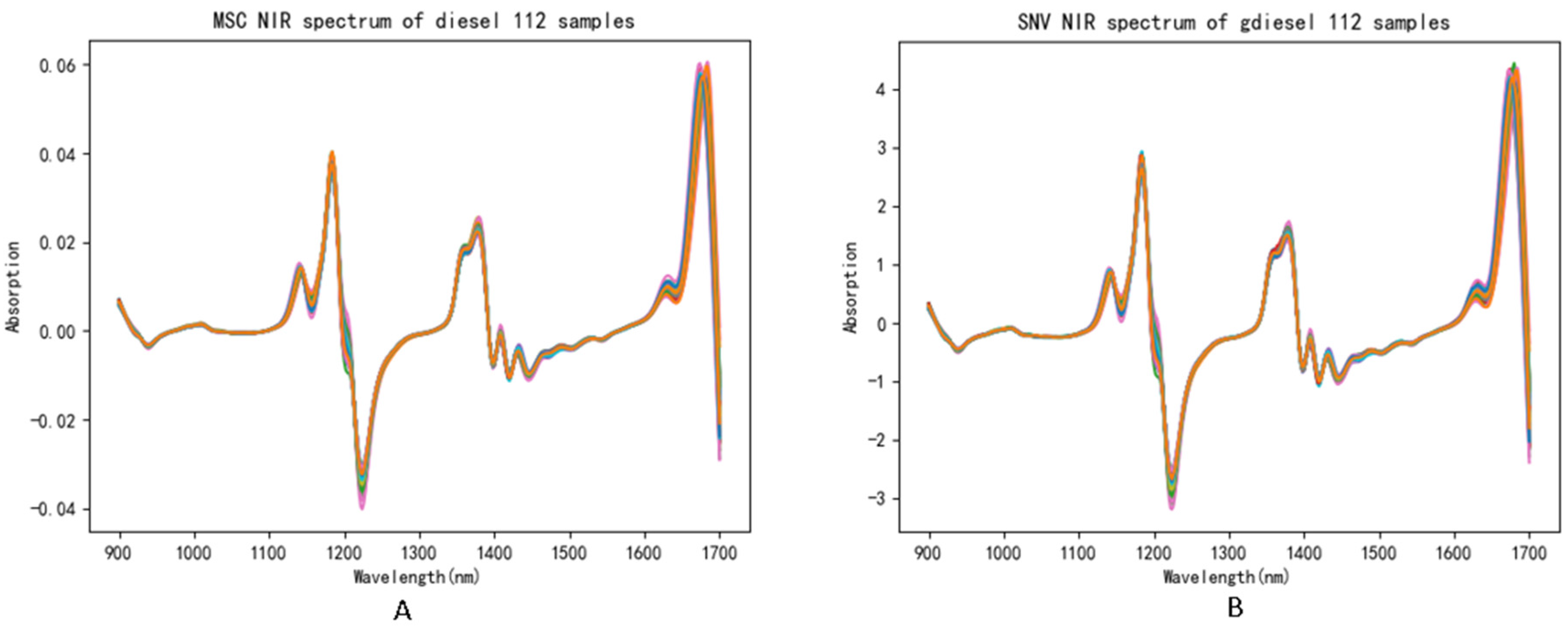
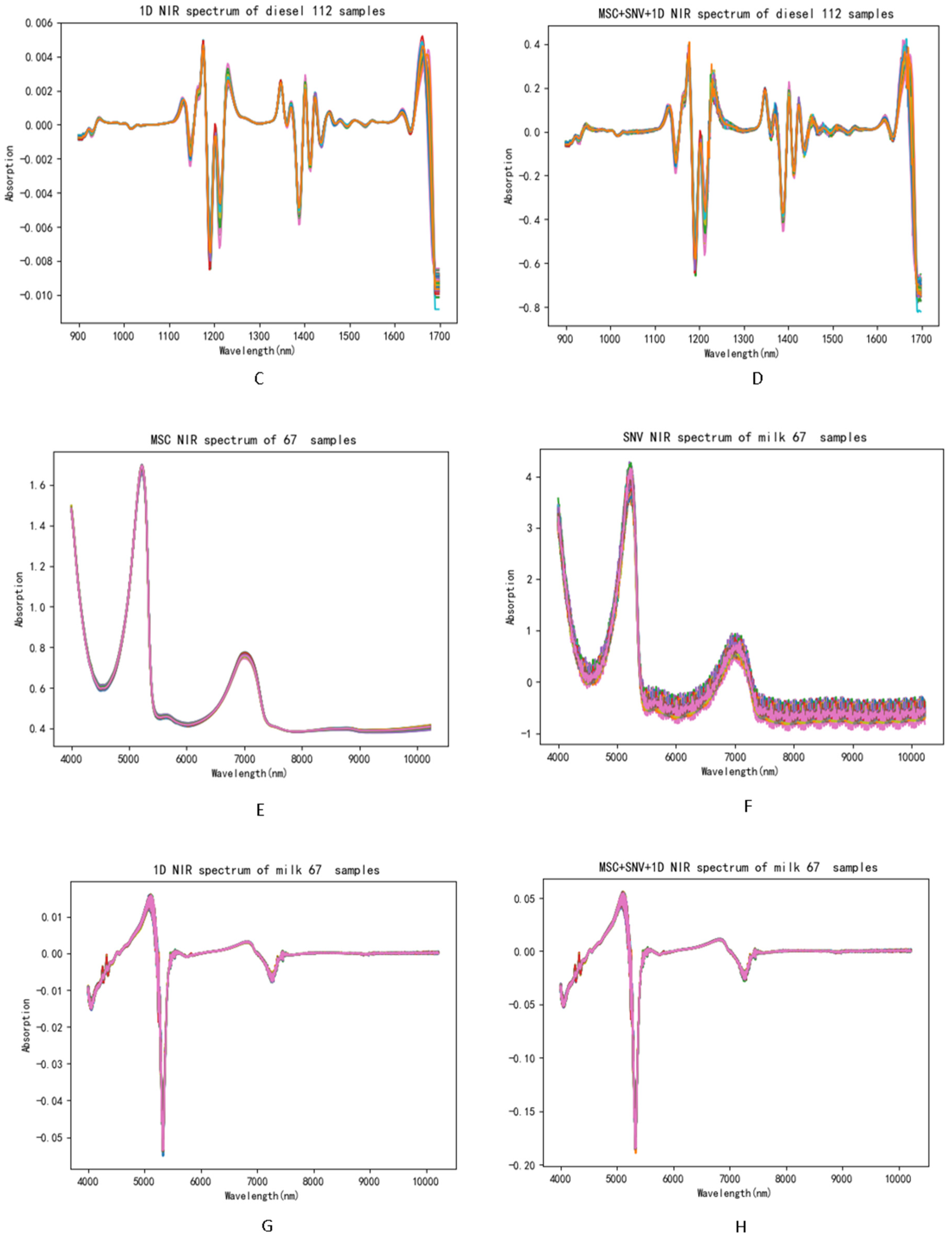
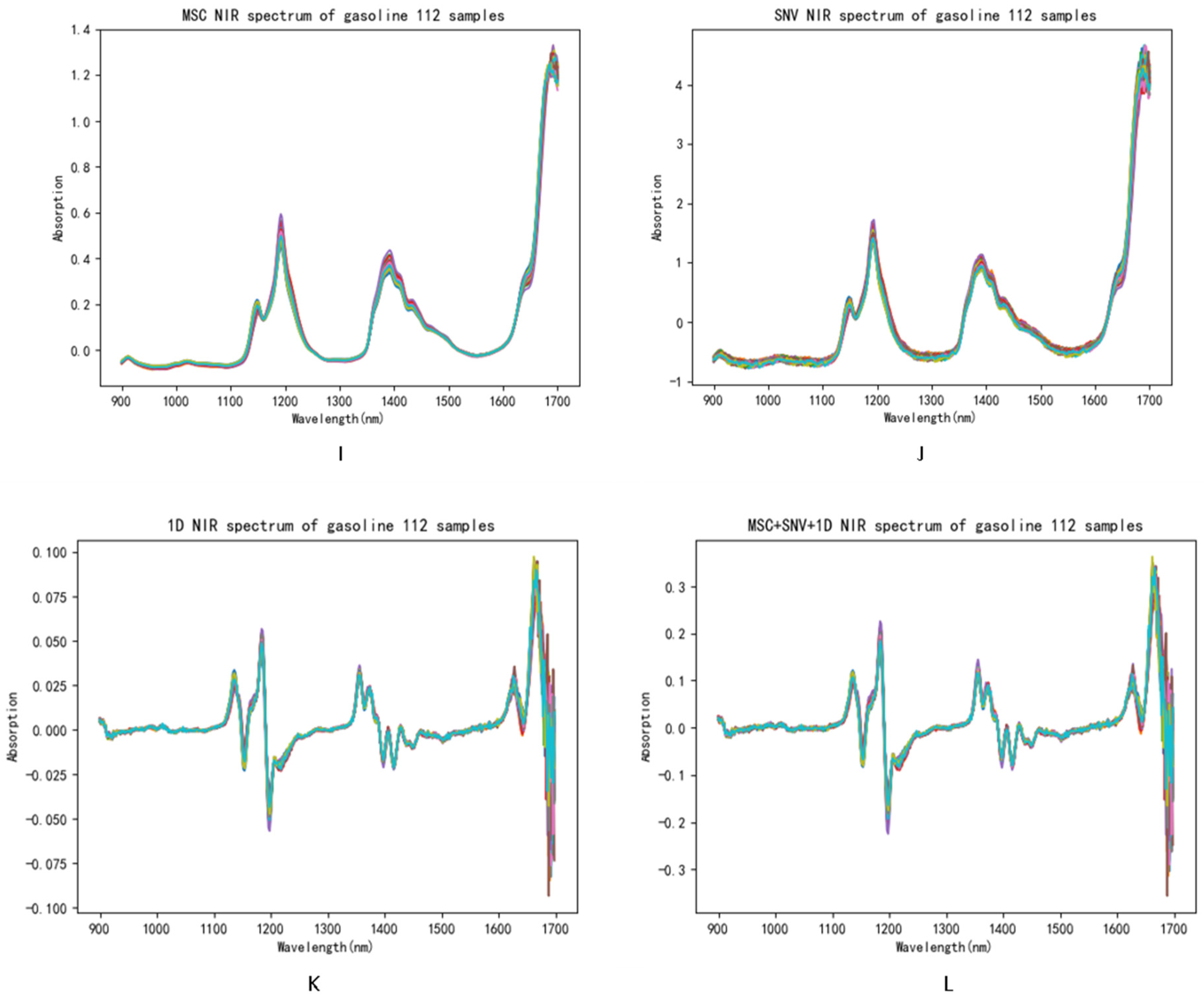
		MSC + SNV + 1D + SVM	0.883699	0.313099

. The results indicate significant variability in the impact of preprocessing on the different samples. Not all preprocessing combinations enhance the accuracy of predictions compared to those made with individual preprocessing techniques. For instance, in the case of the diesel sample analysis, predictions made post-MSC preprocessing alone exhibited a 12.44% higher accuracy than those made after combined preprocessing. Therefore, it is imperative to select preprocessing methods that are tailored to the specific characteristics of each sample.

Table 2 reveals that applying a combination of the three preprocessing methods prior to SVM modeling significantly enhances the predictive accuracy for the cetane number in diesel, octane number in petroleum, and protein content in milk compared to using each preprocessing method in isolation. The R² values for the combined MSC + SNV + 1D + SVM approach outperformed those of the standalone SVM, MSC + SVM, SNV + SVM, and 1D + SVM approaches, achieving values of 0.651380, 0.875780, and 0.883699, respectively. These results indicate performance improvements of 7.96%, 12.48%, and 14.32%, respectively, over the conventional SVM method, underscoring the efficacy of the combined preprocessing approach in regression training. Figure 6 illustrates the training outcomes of the predictive models for the three analytes.

Figure 6 displays the test results of a SVM model with preprocessing applied to three distinct types of samples. The figure is subdivided into six panels, each illustrating different aspects of model performance.

Figure 6A,B focus on the analyte CN-16. In Figure 6A, a scatter plot showcases the relationship between the actual and predicted values, with an R² value of 0.636611, indicating a moderate positive correlation. The line of best fit emphasizes the trend in the data points. Figure 6B presents a line graph detailing both the actual and the adjusted predicted values over a sequence of data points, with an RMSE of 1.839059, providing insight into the model’s prediction accuracy across the dataset. For the analyte octane, panels 6C-D depict similar trends. 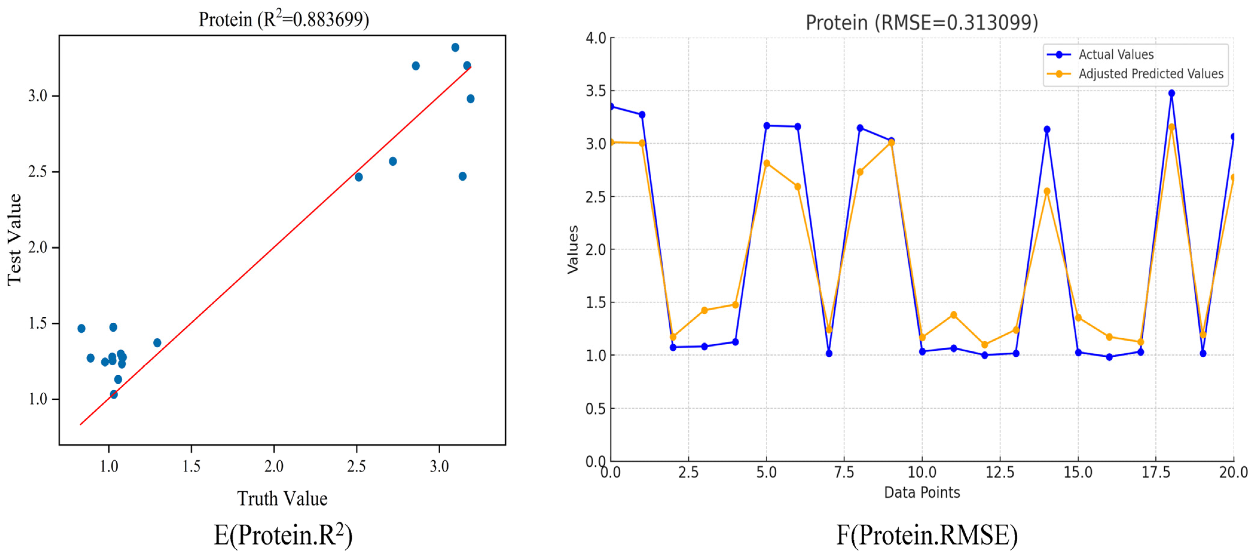Figure 6C’s scatter plot, with an R² value of 0.875788, suggests a strong positive correlation between the true and predicted values, with a closely adhering line of best fit. In panel 6D, the line graph compares the actual and adjusted predicted values with an RMSE of 0.512449, which is lower than that of CN-16, indicating a higher prediction accuracy for octane. Lastly, panels 6E-F represent the analyte protein. The scatter plot in panel 6E, with an R² value of 0.836699, demonstrates a strong correlation between the predicted and actual values. The line of best fit shows the model’s effectiveness at capturing the relationship. Figure 6F’s line graph, with an RMSE of 0.313099, suggests that the model’s predictions are quite precise, as indicated by the lowest RMSE among the three analytes.

Overall, these panels collectively indicate the effectiveness of the SVM model’s predictive capabilities, with varying degrees of accuracy and correlation strength across different analytes. The use of preprocessing techniques appears to enhance the model’s performance, as reflected in the relatively high R² values and lower RMSE scores.

3.3. Training Results of the BEST-1DConvNet Model

The evaluation of the BEST-1DConvNet model, tailored for near-infrared spectroscopy data analysis, revealed significant findings. The model’s architectural optimization, achieved through Bayesian optimization techniques, focused on the fine-tuning of several key hyperparameters, notably enhancing its performance and generalization capabilities. Essential hyperparameters such as the number of convolution layers, the count of convolution kernels, their size, and stride each crucially contribute to the model’s efficacy. The convolution layers’ quantity directly influences the model’s depth and complexity, with a larger number potentially boosting feature extraction capabilities, albeit with an increased overfitting risk. The convolution kernels’ quantity and dimensions affect the range and types of features identifiable by the model at certain layers, thus impacting its recognition and generalization skills. Stride selection affects the spatial resolution of the feature maps, a factor critical to the model’s precision in processing input data details.

In addressing overfitting risks during training, the adoption of an early-stopping strategy was observed—if the loss on the validation set failed to decline significantly over a predetermined number of iterations, training was concluded prematurely. This method not only conserved time and computational resources but also curbed overfitting. The RMSE was deployed as the loss function for gauging the model’s predictive error, while the coefficient of determination (R²) was utilized as the performance metric.

Table 3. Bayesian hyperparameter search parameter ranges.

Parameter Name	Parameter Range
Number of Convolution Layers	1–5
Number of Convolution Kernels	1–28
Convolution Kernel Size	1–517
Convolution Kernel Stride	1–517
Learning Rate	10−6–10−1
Number of Network Layers	1–10

,

Table 4. 1D-CNN Model structure and parameters based on diesel.

Layers	Size	Number	Stride	Kernel Size	Output Shape
Input	1 × 401	-	-	-	-
Conv1	1 × 401	156	494	355	156 × 1
ReLU	-	-	-	-	156 × 1
MaxPooling	156 × 1	-	1	1	156 × 1

,

Table 5. 1D-CNN model structure and parameters based on gasoline.

Layers	Size	Number	Stride	Kernel Size	Output Shape
Input	1 × 401	-	-	-	-
Conv1	1 × 401	16	100	201	16 × 3
ReLU	-	-	-	-	16 × 3
MaxPooling	16×3	-	1	3	16 × 1

and

Table 6. 1D-CNN model structure and parameters based on milk.

Layers	Size	Number	Stride	Kernel Size	Output Shape
Input	1 × 1557	-	-	-	-
Conv1	1 × 1557	14	316	67	14 × 5
ReLU	-	-	-	-	14 × 5
MaxPooling	14 × 5	-	1	5	14 × 1

elucidate the parameters of the convolutional layers for the 1D-CNN and for the diesel, gasoline, and milk datasets, respectively. These tables display the optimal model parameter configurations for the respective datasets, evidencing the BEST-1DConvNet model’s efficacy in NIRS data analysis.

Table 4 and

Table 7. 1D-CNN model R² value and RMSE value.

Dataset Name	R2	RMSE
CN-16	0.968785	1.8223934
Octane	0.975043	0.4951790
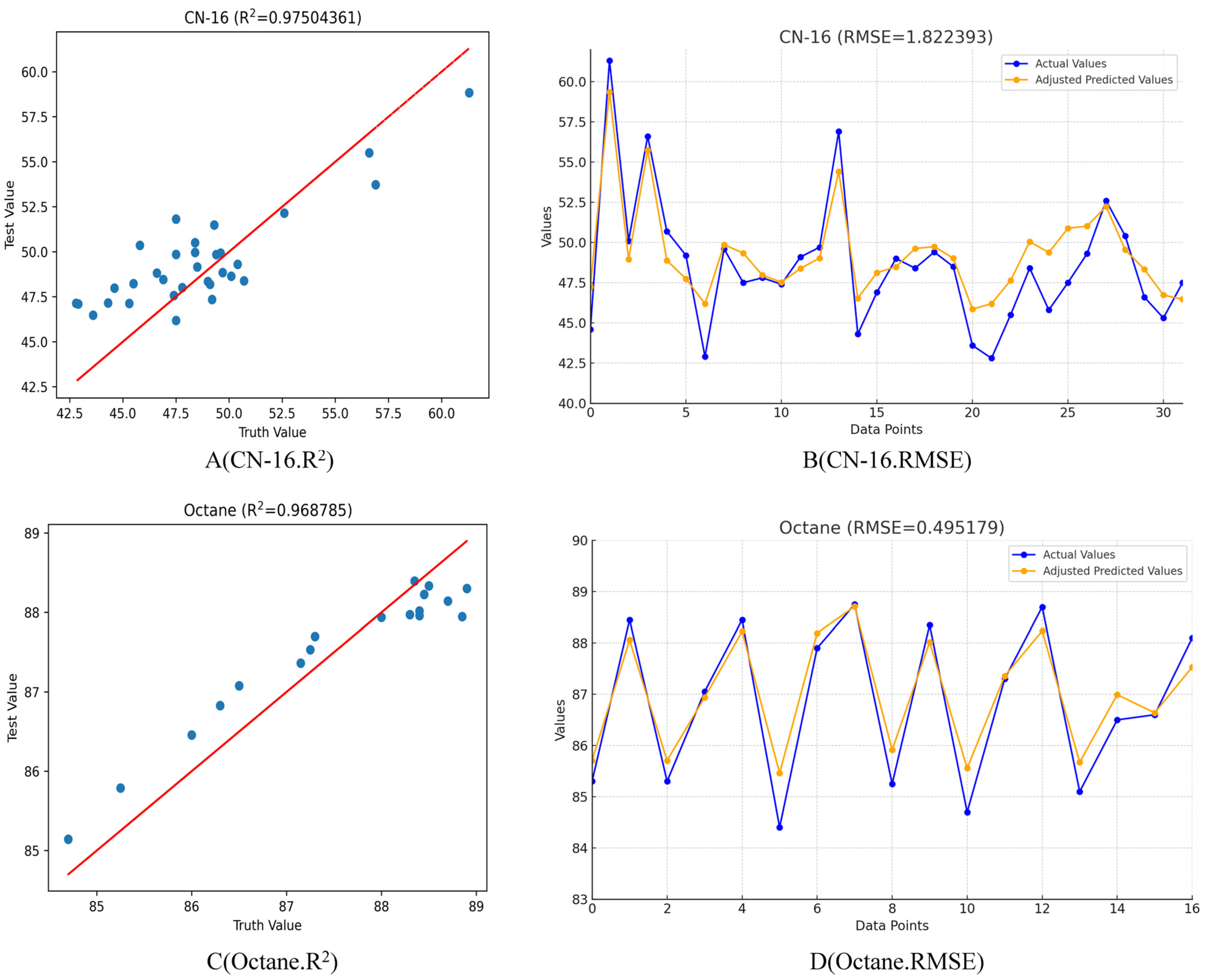
Protein	0.9609851	0.3015460

reveal that after conducting Bayesian hyperparameter search permutations, the CN value prediction model for gasoline comprises a single convolutional layer with a kernel size of 355, 156 filters, a stride of 494, and a learning rate of 0.02289. Training was halted at epoch 160, resulting in an R² value of 0.96878574419 and RMSE of 1.8223934 for the diesel CN value model, as illustrated in Figure 7A, B. Similarly, Table 5 and Table 7 indicate that the cetane-number model for gasoline, derived from a Bayesian hyperparameter search, consists of a single convolutional layer with a kernel size of 201, 16 filters, a stride of 100, and a learning rate of 0.01. Training ceased at epoch 140, yielding an R² value of 0.97504361 and RMSE value of 0.49517905 for the gasoline octane model, as depicted in Figure 7C, D. Finally, Table 6 and Table 7 show that the protein-value model for milk, based on the Bayesian hyperparameter search, consists of a single convolutional layer with a kernel size of 67, 14 filters, a stride of 316, and a learning rate of 0.02289. The training concluded at epoch 200, with the milk protein value model achieving an R² value of 0.96098518661 and RMSE of 0.301546, as shown in Figure 7E, F.

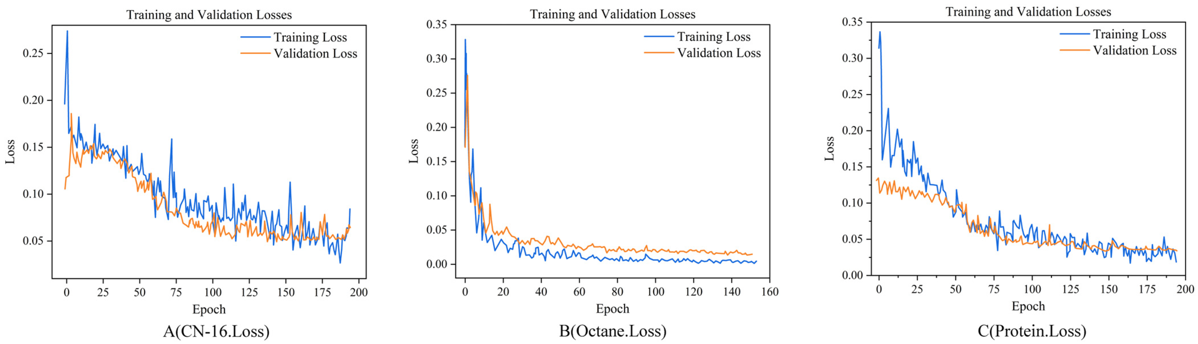
The loss curve graphs show variations in the loss function values of the model during the training process. Each graph comprises two lines: one representing the training loss (blue) and the other representing the validation loss (orange). Ideally, the loss curve should continuously decrease with the progress of training and stabilize towards the end of the training process. In Figure 8A–C, the loss curves demonstrate a reduction in the loss function values as the training progressed, which stabilized after a certain number of iterations. This indicated that the models learned and progressively fitted the data. The close similarity of the training and validation loss curves suggests that the models do not suffer from overfitting and exhibit good generalization capabilities for unseen data. In all three datasets, the rapid decline in the loss curves reached a plateau phase, particularly in Figure 8A, B, where the loss curves stabilized after approximately 50 training epochs. In Figure 8B, this plateau phase appeared earlier, with the loss becoming extremely low and stable after approximately 20 epochs. These indicate that the model quickly captured the key features of the data for the gasoline dataset, whereas, for the other two datasets, more training time might be required to achieve similar levels of performance.

3.4. Model Comparison

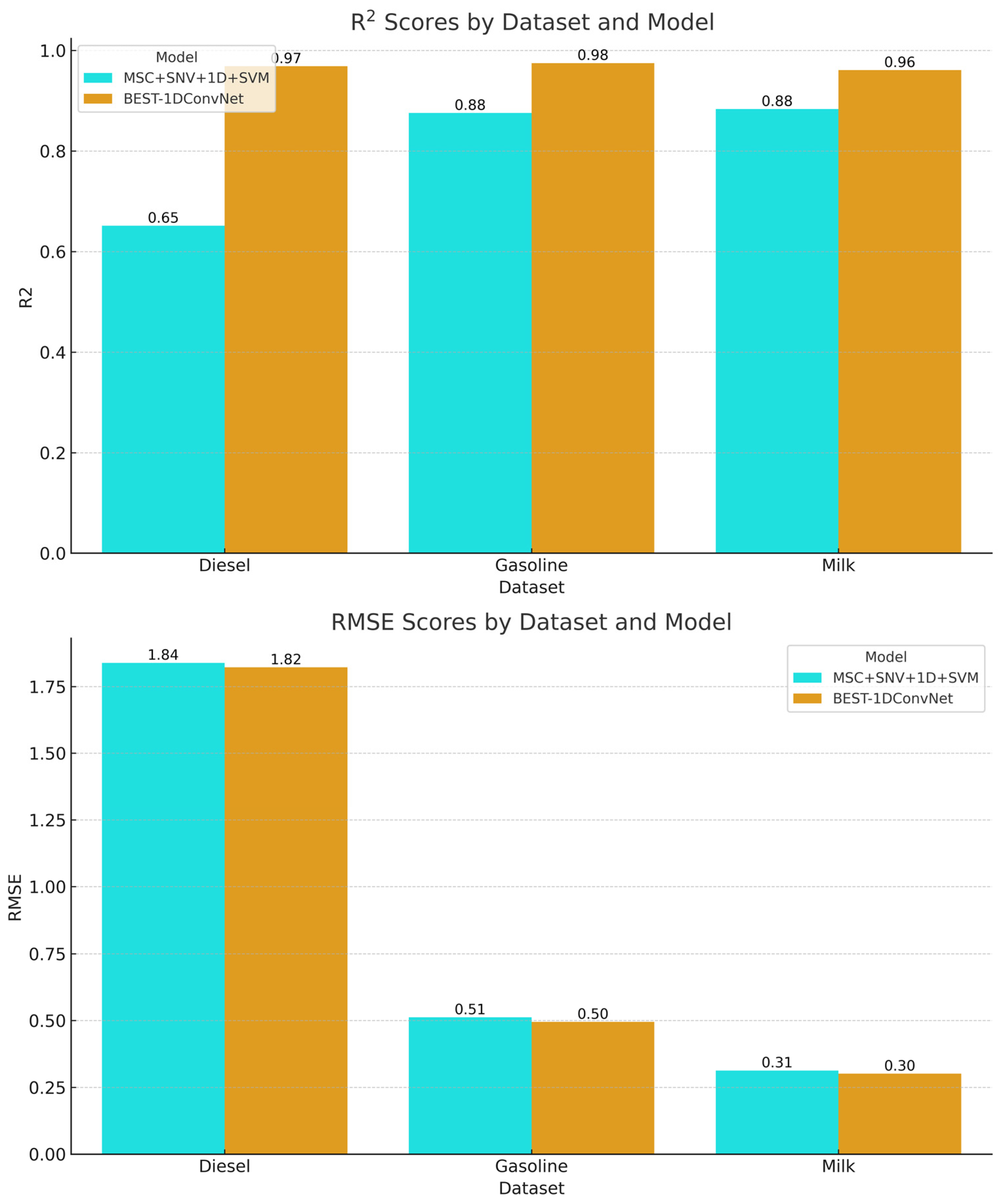
The R² scores, which indicate the explanatory power of the models, were higher for the BEST-1DConvNet model across all datasets, signifying a stronger correlation between the predicted and actual values. For diesel, the R² score was 0.969 for BEST-1DConvNet and 0.651 for MSC + SNV + 1D + SVM. For the gasoline dataset, BEST-1DConvNet achieved an R² of 0.975, whereas the combined preprocessing SVM approach achieved a value of 0.876. The milk dataset results exhibited a similar trend to that of BEST-1DConvNet at 0.961 R², outperforming the SVM combination by 0.884.

In terms of the RMSE, which measures the prediction error magnitude, lower scores indicate better performance. The BEST-1DConvNet model consistently exhibited lower RMSE values, demonstrating superior predictive accuracy. Specifically, for the diesel dataset, the RMSE values were 1.839 for MSC + SNV + 1D + SVM and 1.822 for BEST-1DConvNet. Gasoline showed a more notable difference, with an RMSE of 0.512 for the combined SVM and 0.495 for BEST-1DConvNet. The milk dataset reflected the closest RMSE values, with values of 0.313 for the SVM and 0.302 for the BEST-1DConvNet.

Overall, the bar chart in Figure 9 elucidates the superior performance of the BEST-1DConvNet model over the SVM with preprocessing in both the R² and RMSE metrics, emphasizing its efficacy and precision in predictive tasks within the scope of the analyzed datasets.

4. Discussion

This study primarily investigated the performance of the BEST-1DConvNet model in comparison to that of the MSC + SNV + 1D + SVM model across various substance samples, including diesel, gasoline, and milk. The core design principle of the BEST-1DConvNet model is its ability to automatically tune the architecture and parameters of a 1D-CNN to meet the analytical demands of different substances, thereby exhibiting remarkable generalization capabilities. Empirical results demonstrate that the BEST-1DConvNet consistently outperforms in terms of data fitting ability (higher R² values) and prediction accuracy (lower RMSE values) across all sample types compared to the traditional MSC + SNV + 1D + SVM model.

These findings not only validate the effectiveness of BEST-1DConvNet in the analysis of various substances but also underscore its capacity to autonomously design optimal parameters. Such adaptability and optimization mechanisms offer a robust tool for handling diverse substance samples and are particularly suitable for applications requiring high precision and generalization capabilities. Future research may further explore the applicability of the BEST-1DConvNet model to a broader range of substance types and more complex datasets, as well as enhance its automatic parameter adjustment mechanism to improve its adaptability and accuracy.

References

1. Miseo, E.; Meyer, F.; Ryan, J. Portable Near-Infrared Spectroscopy in Food Analysis. In Encyclopedia of Analytical Chemistry; Wiley: Hoboken, NJ, USA, 2021. [Google Scholar] [CrossRef]
2. Xia, J.; Huang, Y.; Li, Q.; Xiong, Y.; Min, S. Convolutional Neural Network with Near-Infrared Spectroscopy for Plastic Discrimination. Environ. Chem. Lett. 2021, 19, 2629–2636. [Google Scholar] [CrossRef]
3. Perez, I.M.N.; Cruz-Tirado, L.J.P.; Badaró, A.T.; de Oliveira, M.M.; Barbin, D.F. Present and future of portable/handheld near-infrared spectroscopy in chicken meat industry. NIR News 2019, 30, 26–29. [Google Scholar] [CrossRef]
4. Huang, Y.; Gou, M.-J.; Jiang, K.; Wang, L.; Yin, G.; Wang, J.; Wang, P.; Tu, J.; Wang, T. Recent quantitative research of near infrared spectroscopy in traditional Chinese medicine analysis. Appl. Spectrosc. Rev. 2018, 54, 653–672. [Google Scholar] [CrossRef]
5. Bokobza, L. Some Applications of Vibrational Spectroscopy for the Analysis of Polymers and Polymer Composites. Polymers 2019, 11, 1159. [Google Scholar] [CrossRef]
6. Bingari, H.S.; Gibson, A.; Butcher, E.; Teeuw, R.; Couceiro, F. Application of near infrared spectroscopy in sub-surface monitoring of petroleum contaminants in laboratory-prepared soils. Soil Sediment Contam. Int. J. 2022, 32, 237–251. [Google Scholar] [CrossRef]
7. Su, P.; Liang, W.; Zhang, G.; Wen, X.; Chang, H.; Meng, Z.; Xue, M.; Qiu, L. Quantitative Detection of Components in Polymer-Bonded Explosives through Near-Infrared Spectroscopy with Partial Least Square Regression. ACS Omega 2021, 6, 23163–23169. [Google Scholar] [CrossRef]
8. Aguiar, M.I.; Ribeiro, L.P.D.; dos Ramos, A.P.; Cardoso, E.L. Soil characterization by near-infrared spectroscopy and principal component analysis. Rev. Ciênc. Agron. 2021, 52, e20196825. [Google Scholar] [CrossRef]
9. Stacey, P.; Clegg, F.; Rhyder, G.; Sammon, C. Application of a Fourier Transform Infrared (FTIR) Principal Component Regression (PCR) Chemometric Method for the Quantification of Respirable Crystalline Silica (Quartz), Kaolinite, and Coal in Coal Mine Dusts from Australia, UK, and South Africa. Ann. Work. Expo. Health 2022, 66, 825–826. [Google Scholar] [CrossRef]
10. Wang, S.; Liu, P.; Feng, L.; Teng, J.; Ye, F.; Gui, A.; Wang, X.; Zheng, L.; Gao, S.; Zheng, P. Rapid determination of tea polyphenols content in Qingzhuan tea based on near infrared spectroscopy in conjunction with three different PLS algorithms. Food Sci. Technol. 2022, 42, e94322. [Google Scholar] [CrossRef]
11. Ding, Y.; Yan, Y.; Li, J.; Chen, X.; Jiang, H. Classification of Tea Quality Levels Using Near-Infrared Spectroscopy Based on CLPSO-SVM. Foods 2022, 11, 1658. [Google Scholar] [CrossRef]
12. Jernelv, I.L.; Hjelme, D.; Matsuura, Y.; Aksnes, A. Convolutional neural networks for classification and regression analysis of one-dimensional spectral data. arXiv 2020, arXiv:2005.07530. [Google Scholar]
13. Wang, D.; Tian, F.; Yang, S.X.; Zhu, Z.; Jiang, D.; Cai, B. Improved Deep CNN with Parameter Initialization for Data Analysis of Near-Infrared Spectroscopy Sensors. Sensors 2020, 20, 874. [Google Scholar] [CrossRef]
14. Fouad, Z.; Alfonse, M.; Roushdy, M.; Salem, A.-B.M. Hyper-parameter optimization of convolutional neural network based on particle swarm optimization algorithm. J. Electr. Eng. Comput. Sci. 2021, 10, 3257. [Google Scholar] [CrossRef]
15. Mishra, P.; Passos, D. Multi-output 1-dimensional convolutional neural networks for simultaneous prediction of different traits of fruit based on near-infrared spectroscopy. Postharvest Biol. Technol. 2022, 183, 111741. [Google Scholar] [CrossRef]
16. Ning, J.; Ye, H.; Sun, Y.; Zhang, J.; Mei, Z.; Xiong, S.; Zhang, S.; Li, Y.; Hui, G.; Yi, X.; et al. Study on apple damage detecting method based on relaxation single-wavelength laser and convolutional neural network. Food Anal. Methods 2022, 16, 3321–3330. [Google Scholar] [CrossRef]
17. Yun, Y.-H.; Li, H.-D.; Wood, L.R.E.; Fan, W.; Wang, J.-J.; Cao, D.-S.; Xu, Q.-S.; Liang, Y.-Z. An efficient method of wavelength interval selection based on random frog for multivariate spectral calibration. Spectrochim. Acta Part A Mol. Biomol. Spectrosc. 2013, 115, 227–232. [Google Scholar] [CrossRef]
18. Liu, R.; Liu, J.; Liu, C. Determination of Protein Content of Wheat Using Partial Least Squares Regression Based on Near-Infrared Spectroscopy Preprocessing. In Proceedings of the 2022 6th International Conference on Robotics, Control and Vision (ICRCV), Wuhan, China, 25–27 September 2022; IEEE: New York, NY, USA, 2022; p. 9953240. [Google Scholar] [CrossRef]
19. Meng, Y.; Zhang, Y.; Li, C.; Zhao, J.; Wang, Z.; Wang, C.; Li, Y. Prediction of the Carbon Content of Six Tree Species from Visible-Near-Infrared Spectroscopy. Forests 2021, 12, 1233. [Google Scholar] [CrossRef]
20. Dhillon, A.; Verma, G. Convolutional Neural Network: A Review of Models, Methodologies and Applications to Object Detection. Prog. Artif. Intell. 2019, 8, 85–96. [Google Scholar] [CrossRef]
21. Kavzoglu, T.; Teke, A. Advanced hyperparameter optimization for improved spatial prediction of shallow landslides using extreme gradient boosting (XGBoost). Bull. Eng. Geol. Environ. 2022, 81, 201. [Google Scholar] [CrossRef]
22. Kiranyaz, S.; Avci, O.; Abdeljaber, O.; Ince, T.; Gabbouj, M.; Inman, D.J. 1D convolutional neural networks and applications: A survey. Mech. Syst. Signal Process. 2021, 151, 107398. [Google Scholar] [CrossRef]
23. Narkhede, M.V.; Bartakke, P.; Sutaone, M. A Review on Weight Initialization Strategies for Neural Networks. Artif. Intell. Rev. 2022, 55, 291–322. [Google Scholar] [CrossRef]
24. Chen, H.; Tan, C.; Lin, Z.; Wu, T. Rapid Determination of Cotton Content in Textiles by Near-Infrared Spectroscopy and Interval Partial Least Squares. Anal. Lett. 2018, 51, 2570–2584. [Google Scholar] [CrossRef]
25. Al-Saggaf, U.M.; Botalb, A.; Faisal, M.; Moinuddin, M.; Alsaggaf, A.U.; Alfakeh, S. Constraints on Hyper-parameters in Deep Learning Convolutional Neural Networks. Int. J. Adv. Comput. Sci. Appl. 2022, 13, 439–449. [Google Scholar] [CrossRef]
26. Wu, J.; Chen, X.-Y.; Zhang, H.; Xiong, L.-D.; Lei, H.; Deng, S.-H. Hyperparameter optimization for machine learning models based on Bayesian optimization b. J. Electron. Sci. 2019, 17, 26–40. [Google Scholar] [CrossRef]
27. Miseta, T.; Fodor, A.; Vathy-Fogarassy, Á. Surpassing early stopping: A novel correlation-based stopping criterion for neural networks. Neurocomputing 2024, 567, 127028. [Google Scholar] [CrossRef]
28. Hodson, T.O. Root-mean-square error (RMSE) or mean absolute error (MAE): When to use them or not. Geosci. Model Dev. 2022, 15, 5481–5487. [Google Scholar] [CrossRef]
29. Plonsky, L.; Ghanbar, H. Multiple Regression in L2 Research: A Methodological Synthesis and Guide to Interpreting R2 Values. Mod. Lang. J. 2018, 102, 713–731. [Google Scholar] [CrossRef]
Figure 1. Original spectral signals from three public datasets. (A) Near-infrared spectra of 112 diesel samples. (B) Near-infrared spectra of 60 gasoline samples. (C) Near-infrared spectra of 67 milk samples. The x-axis represents the spectral wavelength, while the y-axis denotes the original absorbance values.
Processes 12 00272 g001
Figure 2. Near-infrared (NIR) spectra of three public datasets following preprocessing with Four methods. (AD) display the near-infrared spectra of milk following four different preprocessing methods; (EH) illustrate the near-infrared spectra of diesel after undergoing four types of preprocessing; (IL) depict the near-infrared spectra of gasoline processed with four distinct methods. In all these figures, the horizontal axis represents the spectral wavelength, while the vertical axis denotes the original absorbance values.
Processes 12 00272 g002aProcesses 12 00272 g002bProcesses 12 00272 g002c
Figure 3. Flowchart of NIR spectral data processed by convolutional neural network.
Processes 12 00272 g003
Figure 4. Convolution operation mode between original near−infrared spectrum and convolution kernel function.
Processes 12 00272 g004
Figure 5. BEST-1DConvNet framework structure.
Processes 12 00272 g005
Figure 6. Illustrates the testing performance of the highest-performing support vector machine (SVM) models, which underwent preprocessing, on three distinct types of sample test sets. Specifically, (A,B) represent the scatter and line plots for the actual versus predicted values of CN-16; (C,D) detail the scatter and line plots for octane’s actual versus predicted values. Lastly; (E,F) show the scatter and line plots for protein’s actual versus predicted values, respectively.
Processes 12 00272 g006aProcesses 12 00272 g006b
Figure 7. Visualization of predictive performance and outcomes for the BEST-1DConvNet model: Panels (A,B) display the diesel cetane number model’s R-squared scatter plot and RMSE line graph, respectively; panels (C,D) illustrate the gasoline octane value model’s R-squared scatter plot and RMSE line graph; panels (E,F) depict the milk protein model’s R-squared scatter plot and RMSE line graph.
Processes 12 00272 g007aProcesses 12 00272 g007b
Figure 8. Depiction of the loss function trajectories for the BEST-1DConvNet model: (A) loss curves for both the training and validation sets of the diesel CN-16-number model; (B) loss curves for the training and validation sets of the gasoline octane-value model; and (C) loss curves for the training and validation sets of the milk protein model.
Processes 12 00272 g008
Figure 9. Performance comparison of the support vector machine (SVM) approach combined with preprocessing methods (MSC, SNV, and 1D) against the BEST-1DConvNet model across three different datasets: diesel, gasoline, and milk.
Processes 12 00272 g009