CFD Modeling and Experimental Validation of the Flow Processes of an External Gear Pump

Abstract

This article presents computational fluid dynamics (CFD) modeling of the flow processes at a certain specimen of an external gear pump. The purpose of the developed two-dimensional (2D) CFD model is to carry out a numerical study to obtain the main characteristics of the pump flow rate, especially the flow rate as a function of the pressure and the flow rate as a function of the time. A numerical study was carried out at forty-two different operating modes that were expressed as a variation of two parameters: rotational frequency (950–1450 min⁻¹) and pressure (5–150 bar). The validation of the numerical results was carried out through an experimental study. For this purpose, a laboratory experimental setup equipped with a modern data acquisition (DAQ) system was designed and implemented. It allows the gear pump to be tested at the same operating modes as the numerical study. A validation analysis was performed by comparing the numerical and experimental results using the average relative error index (FIT). A detailed description of the 2D CFD model development (CAD model, mesh, general settings, boundary conditions, etc.) is provided. Based on the 2D CFD model, an original methodology was proposed to take into account the influence of the discharge channels on the displacement volume of the pump by adjusting the face width of the gears. Despite the limitations of the simple 2D CFD model, which are discussed in this article, a very good match between numerical and experimental results is analyzed by calculating the FIT level, which is in the range of 93–97%.

1. Introduction

The characteristic features of rotary displacement gear pumps are their relatively simple construction, small overall dimensions, and mass. There are designs with two, three, or more gears that are meshed externally or internally. External gear pumps are more common. They are widely used in hydraulic drives with both industrial and mobile applications [1]. Their construction consists of two identical spur gears that are placed in a common housing and permanently meshed. One of the gears is driving—it is mounted on a shaft (most often a shaft gear), which passes outside the housing. The other gear is driven from the driving gear. The radial and axial clearances between the gears and the housing are very small. The profile of the teeth is most often involute [2].

The advantages of the external gear pumps are their significantly lower cost (compared to other types of rotary displacement pumps), the possibility of working with relatively unfiltered hydraulic oil, the possibility of combining up to three pumps (with different fixed displacement volumes) driven by one shaft, and the possibility this type of machines to be realized as hydraulic motors. The disadvantages are the relatively high level of the flow rate ripple, noise, fixed displacement volume, impossibility of continuous operation at high pressures (over 25 MPa), and limited repair possibilities. Overcoming these disadvantages has motivated continuous research and development, both by scientific and manufacturing organizations.

There is a large amount of research and development on external gear pumps, which can be summarized in several main directions. A major part of the research is aimed at the influence of the number of teeth, their geometric profile, and contact on the level of the flow ripple [3,4,5,6,7]. A lot of research is aimed at improving the noise characteristics of sound pressure level (SPL), sound intensity, etc. [8,9,10,11,12,13,14,15]. The reason is the existing standards [16] define these characteristics only for the pump as an independent source of noise tested in an anechoic chamber but not for researching the noise characteristics during the operation of the pump in a hydraulic power unit at a normal working environment, with few exceptions [17]. On the other hand, through constructive (design) improvements, the volumetric efficiency could be increased, and this, in turn, motivated a number of studies focusing on gap sizes with the aim of reducing the internal volumetric losses (leakages) [18,19,20,21,22,23]. Although fewer in number, there is research and development related to increasing the high-pressure performance of external gear pumps, which use numerical fluid–structural analysis [24,25,26]. This has led to another part of research aimed at the influence of the trapped volume, inter-teeth pressure, and force distribution on the main (operating) characteristics [27,28,29,30,31]. A separate group of studies is oriented to cavitation phenomena, especially in the meshed zone of gears [6,22,26,32,33,34,35,36,37]. Last but not least, there are studies related to some specific applications of gear pumps [38,39,40,41].

All the listed research directions use numerical modeling to solve a specific task. Earlier studies are based on a one-dimensional (1D) model obtained by an analytical or semi-empirical approach [42]. Gradually, with the development of computational resources, software products are also developed that enable the solution of fluid–structural problems with 2D and three-dimensional (3D) models [43,44,45]. This led to the establishment of a whole scientific field called computational fluid dynamics (CFD), which has also found application in the study of external gear pumps. Due to specifics in the displacement pumps, specialized CFD software products are more often used than general application ones.

In a large part of the research, the development of the CFD model based on constructed geometry is not considered, and in the case of gear pumps, obtaining an adequate model of the flow processes is a difficult task. In addition, the methodology of its creation is hardly considered. This motivated the authors to create such a model using widespread universal software and describe the steps of its creation. Furthermore, in a large part of studies [4,19,23,24,27,28], the geometry is assumed to be known, for example, by the manufacturer. In contrast, in this particular study, it was obtained by measuring and depicting with a digital microscope. On the other hand, a large part of numerical studies [4,5,18,19,27,29,37] lacks validation and verification of the results and the model. This further motivates the authors to create a laboratory experimental setup and data acquisition (DAQ) system to measure the main energy variables (pressure and flow rate) in different modes of pump operation.

The main goal of the article is to develop a 2D CFD model of the flow processes at a certain specimen of the external gear pump. The model’s purpose is to carry out a numerical study to obtain the main characteristics of the pump flow rate, especially the flow rate as a function of the pressure q(Δp) and the flow rate as a function of the time q(t). A numerical study was carried out in different pump operating modes, which are expressed as a variation of two parameters: rotational frequency and load pressure. Validation of the results was carried out through an experimental study. For this purpose, a laboratory experimental setup with a modern DAQ system was designed and implemented. It allows the gear pump to be tested in the same operating modes as the numerical study. The validation analysis was performed by comparing the numerical and experimental results using FIT. A detailed description of the 2D CFD model development can serve as a basis for the creation of such models by other authors for different types of hydraulic machines since such descriptions are missing in a large part of the literature. The resulting 2D CFD model will be further enhanced and used in future studies of noise and vibration processes in the pump discharge pipeline.

This article is organized as follows. Section 2 includes a detailed description of CFD model development, Section 3 presents the obtained numerical results, Section 4 shows the experimental system layout, Section 5 consists of the experimental validation of the numerical results, and in Section 6, some conclusions are given.

2. CFD Model Development

The object of the present study is a certain specimen of an external gear pump with no design information (both geometrical description and test results) available. Preliminary laboratory tests were conducted, and the pump flow rate was measured as 26.7 L/min in nominal operation mode at a pressure of Δp = 150 bar and a rotational frequency of n = 1450 min⁻¹.

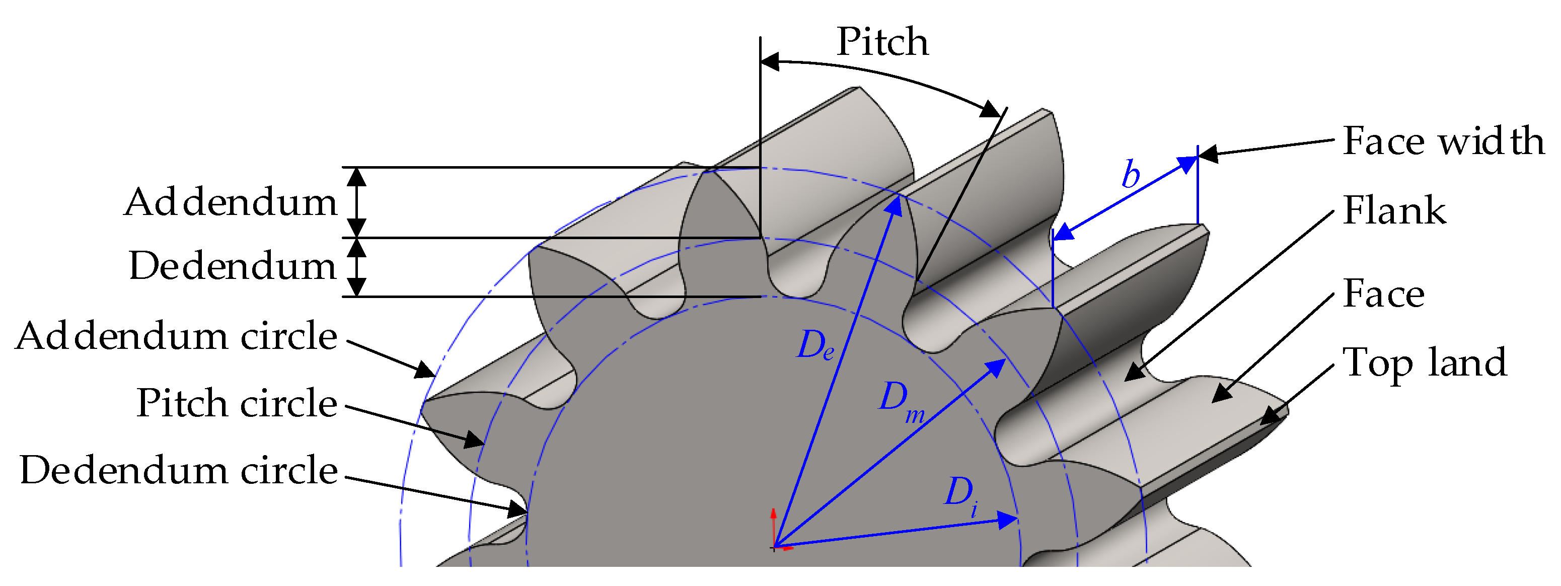
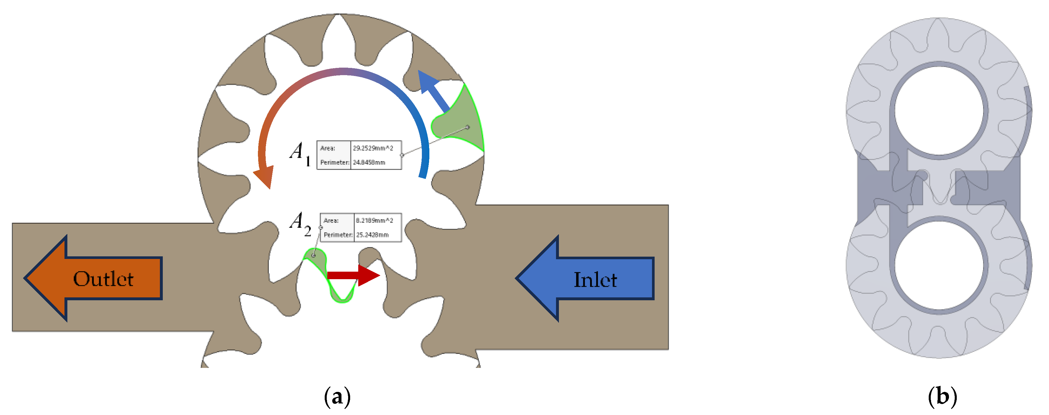
2.1. Determination of the Pump Displacement Volume

The main elements in external gear pump construction are two identical spur gears, most often having an involute profile. The terminology related to their design parameters, established in the literature [46], is shown in Figure 1.

There are two approaches for determining the gear pump displacement volume based on the design parameters of the spur gears: geometric and parametric [47,48,49]. Both approaches are valid only if the following assumptions are accepted:

• Gears without correction factors;
• Teeth number in range of z = 9–14;
• Center distance between the two gears a is equal to the pitch circle diameter D_m;
• The area of one tooth is equal to the area between two consecutive teeth.

2.1.1. Geometric Approach

The displacement volume V_g of the external gear pump can be expressed by:

$$\begin{array}{l}{V}_g=2\left(\frac{\pi D_e^2}{4}-\frac{\pi D_i^2}{4}\right)\frac{b}{2}=\frac{\pi }{4}b\left(D_e^2-D_i^2\right)\\ =\frac{\pi }{4}b\left(D_e+D_i\right)\left(D_e-D_i\right)=\frac{\pi }{2}b\left(\frac{D_e+D_i}{2}\right)\left(D_e-D_i\right)\end{array},$$

(1)

where D_e is the addendum circle diameter, D_i is the dedendum circle diameter, b is the face width, and (D_e + D_i)/2 = D_m = a. Therefore, (D_e − D_i)/2 = D_e − D_m = D_e − a. By substituting the above expression, we obtain:

$$V_g=\frac{\pi }{2}ba\left(D_e-D_i\right)=\pi ba\left(\frac{D_e-D_i}{2}\right)=\pi ba\left(D_e-a\right).$$

(2)

2.1.2. Kinematic Approach

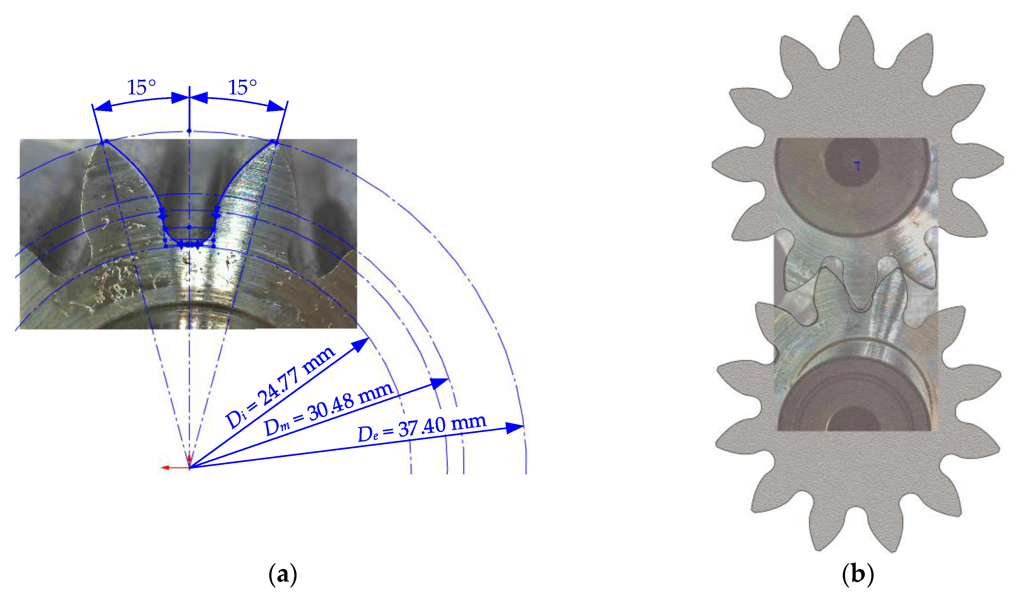
To determine the displacement volume V_k of an external gear pump expressed by the flow rate, the kinematic approach is used.

The flow rate q of the external gear pump can be determined by:

$$q=b\left(\frac{D_e-D_i}{2}\right)\omega \left(\frac{D_m}{2}\right)=\frac{2\pi n}{60}b\frac{D_m}{2}\left(D_e-a\right),$$

(3)

where the diameter of the pitch circle is D_m = a, (D_e − D_i)/2 = D_e − D_m = D_e − a, and ω is the rotational frequency. Then, the displacement volume V_k is:

$$V_k=\pi ba\left(D_e-a\right),$$

(4)

since the flow rate of the pump is $q=V_k\frac{n}{60},\frac{{\mathrm{m}}^3}{\mathrm{s}}$.

In the theory and practice of hydraulic displacement machines, another way to determine the displacement volume is often used, which gives very close results to the one expressed above:

$$V_p=k\pi D_{m}2mb,$$

(5)

Where k = 1.035 is the tooth height factor [50] and m is the gear module. This value is valid provided that the last prerequisite is met—the area of one tooth is equal to the area between two consecutive teeth. Therefore, the displacement volume V_p of the pump is:

$$V_p\approx 6.5D_{m}mb.$$

(6)

The displacement volume of the investigated pump was determined according to the three presented dependencies, which gave a very close result, approximately equal to 19 cm³. The design parameters are determined by a preliminary micrometer measurement of the pump details.

2.2. CAD Model

One of the main challenges in CFD models’ development is specifying the geometry. In our specific case, the following techniques were used:

• Measurements with an accuracy of 0.01 mm;
• High-resolution photography with a digital microscope;
• The dimensions are partly calculated, and involutes are plotted according to the well-known formulas in machine element design theory [46]. They are derived from the number of teeth z and the diameters of the addendum and dedendum circles (D_e and D_i);
• CAD model creation in SolidWorks^® 2019 SP5.0 Education Edition environment with the imposition of sketches on the captured images (Figure 2a);
• A comparison of the resulting tooth profile with high-resolution photographs at the same scale shows satisfactory results—see Figure 2b.

Due to the relatively simple construction, the measurement, geometrical construction, and assembly of the remaining parts did not cause difficulties, except for the definition of the radial and axial gaps, which are important for further models and analyses. After careful measurement and based on the available information for this class of pumps, it was assumed that:

• Radial gap: 0.02 mm;
• Axial gap: 0.025 mm.

A clearance in the tooth meshing of 0.0092 mm was added to these two types of clearances. In reality, such a gap does not exist, and the teeth are in direct contact with each other. However, it is necessary for the creation of a dynamic mesh, which is needed in the chosen approach of CFD simulations.

The literature survey [4] showed that the most commonly used value is 0.01 mm. A clearance of this size is small enough that no significant amount of fluid passes through it from the high- to the low-pressure area to affect the results. Reducing the clearance below this value causes numerical solution problems due to the extremely small size of finite elements between the teeth. Increasing the clearance, on the other hand, reduces the required computational resources but increases the leakages through it.

Figure 3 shows the created CAD model of the pump in a disassembled state.

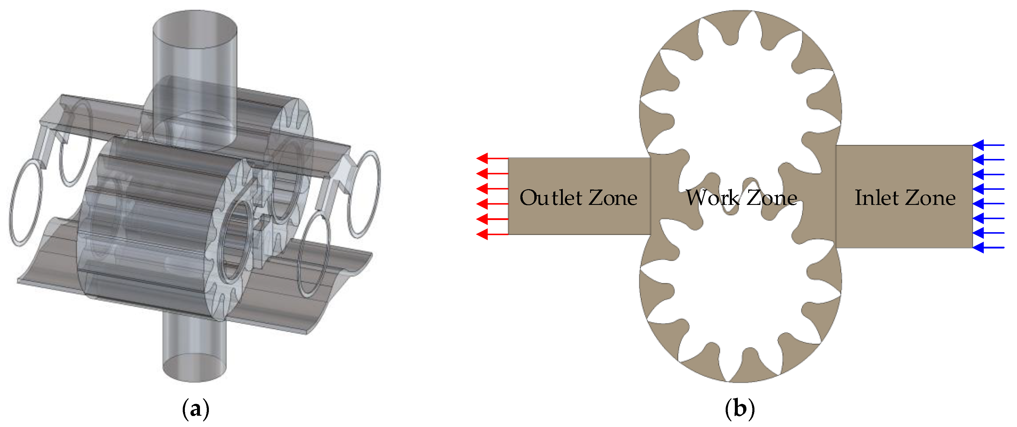
2.3. Development of a Simplified Geometrical Model for CFD Simulations

The development of a detailed pump CAD model allows the full fluid internal volume to be easily obtained, including all channels and gaps. The resulting 3D fluid body (Figure 4a) is very complex. In addition to workspaces, it contains three additional groups of fluid volumes:

• Lubrication channels—with relatively small volume. They are not expected to influence the q(Δp) and q(t) characteristics;
• Channels to ensure more uniform deformation of the bearing bodies and more uniform wear of the bearing sleeves. These channels have a larger volume than the lubrication channels but are located away from the working chamber and are also not expected to have a significant impact on the q(Δp) and q(t) characteristics;
• Discharge channels. They ensure a more even pressure distribution, largely prevent the creation of areas of excessively high or excessively low pressure, reduce the risk of cavitation, and reduce wear. They also increase the displacement volume because they reduce the fluid transfer from the high- to the low-pressure area through the tooth meshing area. The discharge channels’ influence on q(Δp) and q(t) is significant, mainly because of their effect on the pump displacement volume.

The literature review shows that channels in the first two groups are rarely modeled in numerical studies [28]. On the other hand, modeling the discharge channels is mandatory in 3D computational models.

When creating a simple geometric model for CFD simulations, the first step is to decide on its dimensionality—2D or 3D. Two-dimensional models are significantly simpler geometrically, resulting in meshes with a much smaller number of finite elements, which reduces computational time. On the other hand, they cannot account for some important effects, such as the transverse movement of the fluid, especially in the area of the suction and discharge ports, as well as the presence of discharge channels. In the 3D models, these disadvantages are absent, but the resulting meshes usually contain hundreds of times more finite elements. The resulting CFD models often cannot be solved by a modern desktop computer.

The literature survey showed that very often authors limit their numerical experiments to 2D simulations [3,32,33,37]. With proper tuning, these models can also provide the accuracy needed to study some basic operating parameters, such as flow rate. Authors performing 3D simulations very often also start their research with 2D modeling [19,28,29,42]. Once working 2D models are achieved, they transfer established definitions and parameters (e.g., finite element mesh density) to more complex 3D models, significantly reducing final model preparation time. All this gave us a reason, in this initial research, to focus our efforts on 2D simulation.

The 2D geometric model used in the present study is shown in Figure 4b. This model has three zones:

• Suction and delivery ports (Inlet Zone and Outlet Zone in Figure 4b). They do not change their shape and size during operation, which reduces the requirements for the finite elements mesh. It is appropriate to use a structured mesh of rectangular finite elements (quadrilaterals face meshing). This type of mesh gives faster and more stable solutions than other types of meshes, very often and more accurately, due to the even shape of the elements. Larger-size elements can be used without negatively affecting the solution.
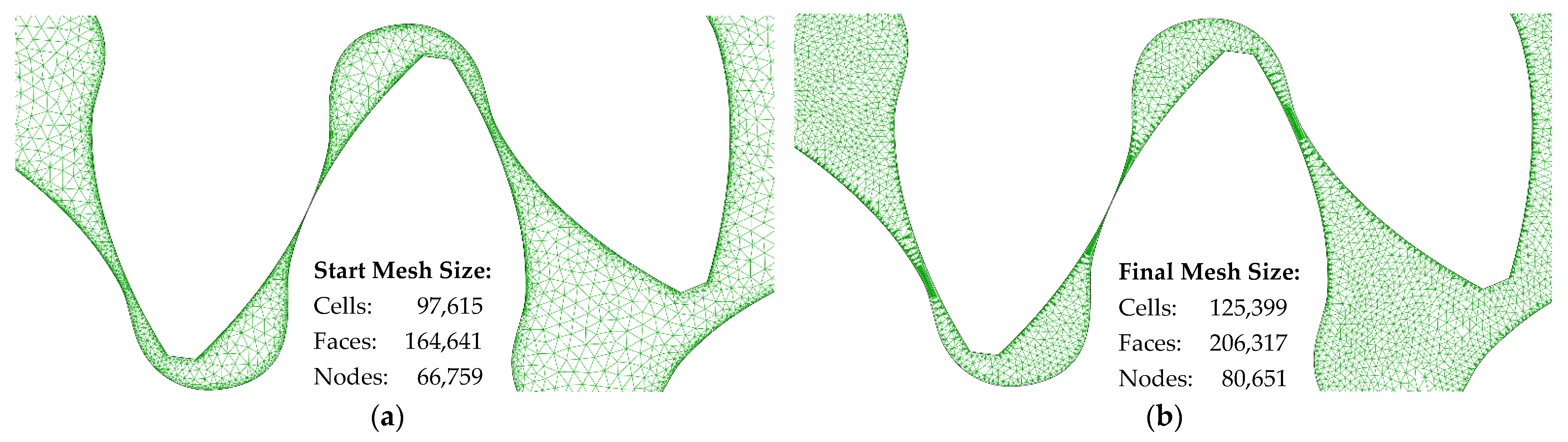
• Work Zone. Due to the movement of the gears, this area changes its shape with each time step. When using a dynamic mesh CFD model, the mesh is regularly adjusted to fit the new geometry. This, in turn, with universal software packages, such as ANSYS Fluent^® 2019 R3, requires the use of an unstructured mesh of triangular finite elements (all triangles method), which allows fast remeshing. To reduce the remeshing time and the risk of numerical errors (typically: floating point exception or negative cell volume), a finer mesh has to be used in this zone than in others.

An important 2D model parameter is the gear face width b. In our 2D model, it is different from the physical face width because through this parameter, the discharge channel influence is taken into account.

In Figure 5a, the areas of the space between two teeth and the outer wall A₁, as well as between the meshed teeth A₂, are outlined and measured. There are two gears, and the mesh is one, for one revolution fluid, is transferred through twenty-four areas A₁ from the Inlet to Outlet, as well as through twelve areas A₂ from Outlet to Inlet. Thus, the 2D model working area is A = 24A₂ − 12A₁. The face width b = V_p/A of the model is calculated to provide the displacement volume of the pump V_p = 19 cm³, which is determined by (5) and (6). Thus, b is found to be approximately equal to 31.5 mm, while the actual measured value of face width b is 30.89 mm. The calculated value of b is larger as a result of the fluid transfer in the opposite direction through area A₂. This transfer is actually smaller due to the presence of discharge channels outside the plane of the simulation, as shown in dark grey color in Figure 5b.

2.4. Theoretical Background of the CFD Model

The implementation of the CFD model is based on some basic dependencies of the computational fluid mechanics [51] embedded in the used software.

The general form of the continuity equation for compressible fluid is:

$$\frac{\partial \rho }{\partial t}+\overrightarrow{\nabla }.(\rho \overrightarrow{V})=0,$$

(7)

where $\rho$ is a density of fluid, $\overrightarrow{V}$ is a velocity vector, and $\nabla$ is divergence (Gauss’s theorem). A particular case is the steady state for compressible working fluid, in which $\frac{\partial }{\partial t}=0$ (for any variables); therefore:

$$\overrightarrow{\nabla }.(\rho \overrightarrow{V})=0.$$

(8)

Assuming that the working fluid is incompressible, it follows that ρ = const; therefore: $\frac{\partial \rho }{\partial t}\cong 0$, and the continuity equation takes the form:

$$\overrightarrow{\nabla }\times \overrightarrow{V}=0.$$

(9)

The incompressible form often is expressed as:

$$\frac{\partial u}{\partial x}+\frac{\partial v}{\partial y}+\frac{\partial w}{\partial z}=0,$$

(10)

where u, v, and w are the velocity components.

For the purposes of computational fluid mechanics, it is more appropriate to represent the Navier–Stokes equations in a Cartesian coordinate system. The Navier–Stokes equation for incompressible fluid has a general vector form:

$$\rho \left(\frac{\partial \overrightarrow{V}}{\partial t}+\left(\overrightarrow{V}\overrightarrow{\nabla }\right)\overrightarrow{V}\right)=-\overrightarrow{\nabla }P+\rho \overrightarrow{g}+\mu {\nabla }^2\overrightarrow{V},$$

(11)

where P is the pressure, μ is the dynamic viscosity, and g is the gravity. It is valid for Newtonian fluid, which has constant properties that are expressed for each of the coordinate axes:

X—the component of the equation is:

$$\rho \left(\frac{\partial u}{\partial t}+u\frac{\partial u}{\partial x}+v\frac{\partial u}{\partial y}+w\frac{\partial u}{\partial z}\right)=-\frac{\partial P}{\partial x}+\rho g_x+\mu \left(\frac{{\partial }^{2}u}{\partial x^2}+v\frac{{\partial }^{2}u}{\partial y^2}+w\frac{{\partial }^{2}u}{\partial z^2}\right).$$

(12)

Y—the component of the equation is:

$$\rho \left(\frac{\partial v}{\partial t}+u\frac{\partial v}{\partial x}+v\frac{\partial v}{\partial y}+w\frac{\partial v}{\partial z}\right)=-\frac{\partial P}{\partial y}+\rho g_y+\mu \left(\frac{{\partial }^{2}v}{\partial x^2}+v\frac{{\partial }^{2}v}{\partial y^2}+w\frac{{\partial }^{2}v}{\partial z^2}\right),$$

(13)

where g_x and g_y are gravity in the x and y directions. Z is a component of the Navier–Stokes equation and is not applicable to the developed 2D CFD model.

There are two main turbulence models according to CFD theory: k-ε and k-ω [51]. The k-ε model is most commonly used to simulate the mean flow characteristics in turbulent flow conditions. It is an Eddy viscosity two-equation model that belongs to the class of turbulence models used to determine the Reynolds stresses. That means that it solves two transport equations for convection and diffusion of turbulent energy in addition to the conservation equations. The two transported variables are turbulent kinetic energy (k), which determines the energy in turbulence, and the turbulent dissipation rate (ε), which determines the rate of dissipation of turbulent kinetic energy. There are variations of the k-ε model such as standard, realizable, and RNG, and their modifications make a better performance of simulations in certain fluid flow conditions possible.

The k-ε model is reliable for free-shear flows, such as the ones with relatively small pressure gradients. It finds application in objects with high Reynolds numbers. The standard model might not be the best model for problems involving adverse pressure gradients, large separations, reattachments, axisymmetric jets, and complex flows with strong curvatures.

The k-ω turbulence model is one of the most commonly used models to evaluate the effect of turbulent flow conditions. It is a part of the Reynolds-averaged Navier–Stokes (RANS) family of turbulence two-equation models, where all the influences of turbulence are modeled. It also solves two transport equations for the convection and diffusion of turbulent energy, in addition to the conservation equations. However, the two transported variables are turbulent kinetic energy (k), which determines the energy in turbulence, and the specific turbulent dissipation rate (ω), which determines the rate of dissipation per unit of turbulent kinetic energy.

The k-ε model uses empirical damping functions in the viscous sub-layer region, which were essentially derived for the flat plate boundary layer flows. In the presence of adverse pressure gradients (e.g., flows past airfoil and turbine blades), it is not very accurate. The k-ω model does not require these damping functions to give a better accuracy. Therefore, the best use for near-wall treatment is the standard k−ω model. However, the k−ω model realizes the best performance for complex boundary layer flows under adverse pressure gradients and separations (e.g., external aerodynamics and turbomachinery). Therefore, for the studied displacement gear pump, it is more appropriate to use a standard k-ε model.

The turbulence k-ε (kinetic energy) equation can be expressed as follows:

$$\frac{\partial }{\partial t}\left(\rho k\right)+\nabla \left(\partial k\overrightarrow{V}\right)=\nabla \left[\left(\mu +\frac{{\mu }_i}{{\sigma }_k}\right)\nabla k\right]+G_k+G_b-\rho \epsilon -Y_M+S_k,$$

(14)

$$\frac{\partial }{\partial t}\left(\rho \epsilon \right)+\nabla \left(\partial \epsilon \overrightarrow{V}\right)=\nabla \left[\left(\mu +\frac{{\mu }_i}{{\sigma }_{\epsilon }}\right)\nabla \epsilon \right]+C_{1\epsilon }\frac{\epsilon }{k}\left(G_k+C_{3\epsilon }{G}_b\right)-C_{2\epsilon }\rho \frac{{\epsilon }^2}{k}+S_k,$$

(15)

where k is the kinetic energy, σ_k is the turbulent Prandtl number for k, ε is the kinetic energy dissipation rate, σ_ε is the turbulent Prandtl number for ε, G_k is the generation of turbulence kinetic energy (mean velocity gradients), G_b is the generation of turbulence kinetic energy due to buoyancy, S_k is the user-defined source terms, and C_1ε, C_2ε, C_3ε, and C_μ are constants.

The Eddy viscosity μ_i is calculated by combining k and ε as follows:

$${\mu }_i=\rho C_{\mu }\frac{k}{\epsilon }.$$

(16)

2.5. Creating a CFD Model

The first step of CFD model creation is to choose the right software. There are two possible approaches:

• Specialized gear pump modeling software. A typical representative is PumpLinx^®;
• Universal CAE software containing modules for CFD simulations. A typical example is the ANSYS^® software package.

Specialized software has the advantage of generating and using structured meshes. This allows us to reduce the required computing resources and solve large 3D CFD models. In addition, the user is offered easily accessible functionalities; for example, gas fraction analysis, in order to investigate the cavitation phenomenon [26,39]. The disadvantage is the need to purchase the product separately.

The main advantage of universal CAE software is that universities and scientific organizations, as well as many engineering companies, already have licenses for such packages, which then can be used without additional cost. The disadvantages are many: they are more complex, require higher qualifications, take more time to build and tune the models, and require more computing resources, time, and experience to reach stable models and solutions. As the Technical University of Sofia has a license for the ANSYS^® Software package, version 2019 R3, it was decided to use this particular software.

The second step is to select an appropriate strategy for the required simulation and a module that can implement it. The conducted studies and trial simulations showed that there are two possibilities:

• Immersed solid method and ANSYS CFX^® module. Although there are not many, solutions using this approach are found in [24]. In this method, there are two separate meshes sharing the same volume: a fluid and a mobile solid immersed in it. The method has the huge advantage that it gives stable solutions on relatively large meshes, which allows us to quickly obtain results in 3D CFD simulations with significant geometries. The disadvantages are also not to be neglected, and they are the reason why this method is not preferred for modeling gear pumps. The main thing is that the phenomena near the walls, at the fluid/gear interface, cannot be accurately modeled.
• Dynamic mesh and ANSYS Fluent^® module. Dynamic mesh is a feature that allows the mesh to deform and adapt to the motion of the boundaries. The method allows defining the size of the elements on the boundaries of the model, general control over the size of the elements generated during the solution (Minimum and Maximum Length Scale), partial control over the elements’ shape (Maximum Cell Skewness), and other settings. This is the preferred method in the literature for gear pump analyses, as it gives the most accurate solutions and allows maximum control in the boundary zones. Its main disadvantage is its resource intensity. Even in 2D, it requires a very fine mesh. In the areas with clearances, the elements have dimensions of the order of 5–20 μm. It requires frequent remeshing, usually at each time step. The time step is extremely small, typically 1 × 10⁻⁶ s in the literature [24], requiring thousands of time steps to be calculated. At least 20 iterations are usually used to calculate each time step. Additionally, using an unstructured mesh of pyramids (3D) or triangles (2D) results in a very large number of elements and nodes. This method is preferred in the present study. With the current setup, with a workstation with an Intel^® Core™ i7-12800H processor and 32 GB RAM, the calculation speed is 100 min/30° in 2D, and the solution in 3D is practically impossible due to insufficient processing power.

The mesh settings have a very significant effect on both the quality and type of the mesh, as well as the calculation time and the solution stability. Only a few time steps after the start, the mesh is different from the initial input, generated with a separate mesh generation module (e.g., ANSYS Meshing™).

Different combinations of parameters and mesh settings were used in the construction of the model to search of an optimal option where the numerical error is minimized and the calculation time (which strongly depends on the number of finite elements) remains acceptable. In addition, the mesh density is related to the time step—a coarse mesh allows for a larger step, so the effect on computation time can be increased.

In the present study, combinations were tried, and solutions were obtained in the range of 50,600 to 187,500 finite elements and time steps from 1e-6 s to 7e-6 s. It is separately checked how the size of the finite elements in the interval of 0.05 mm (1,899,665 finite elements) to 0.25 mm (37,292 finite elements) (away from the walls) affects the computation time.

For meshes with more than 60,000 (up to 187,500) finite elements, no significant influence of the mesh density on the final results is observed. Here, we clarify that in order to obtain stability, the mesh in the contact areas (gaps) is always kept fine, with an element size of 0.013–0.02 mm. Therefore, in the final studies, a mesh with an order of 100,000 finite elements and a time step of 2e-6 s (at 1450 min⁻¹) was used. With these parameters, good solution stability and satisfactory results were obtained, with a relatively low calculation time (about 90 min for 30 degrees).

Figure 6 shows the used mesh and its parameters. A base mesh size of 0.25 mm was used for initial meshing. The mesh is finer in the slack areas and uses 0.013 and 0.02 mm element sizes for the involutes; 0.034 mm for rounding; 0.05 mm for the tips of the teeth; and 0.08 mm for the walls. The Inlet and Outlet Zones have a static structured rectangular mesh with sides of 0.25 mm. As can be seen in Figure 6, with the selected settings after remeshing, the mesh becomes more uniform and has a larger number of nodes. The set sizes along the contours are preserved, while the elements change their shape and density in depth. The literature review showed that usually the general appearance and description of the initial mesh is given, but practically no comment is made on how this mesh changes during the solution.

2.6. General Settings of the CFD Model

The definition of the CFD model in ANSYS Fluent^® 2019 R3 went through the following stages:

• Solver type: Transient;
• Gravity: 9.81 m/s² along Y;
• Viscose model: A standard κ-ε (two-equation type) with standard Wall Functions, as recommended in the literature, is chosen [32]. Model constants used values are
  C_μ = 0.09; C_1ε = 1.44; C_2ε = 1.92; (TKE Prandtl Number) σ_k = 1.0; and (TDR Prandtl Number) σ_ε = 1.3.

• Material: The working fluid is hydraulic oil (HLP 32), for which the following two material properties are set:

  -

  Density: 890 kg/m³;

  -

  Viscosity: 0.0712 kg/(m.s).

• Boundary conditions:

  -

  Inlet: Set to “Pressure Inlet” type, with a pressure of 1 bar, normal to the boundary;

  -

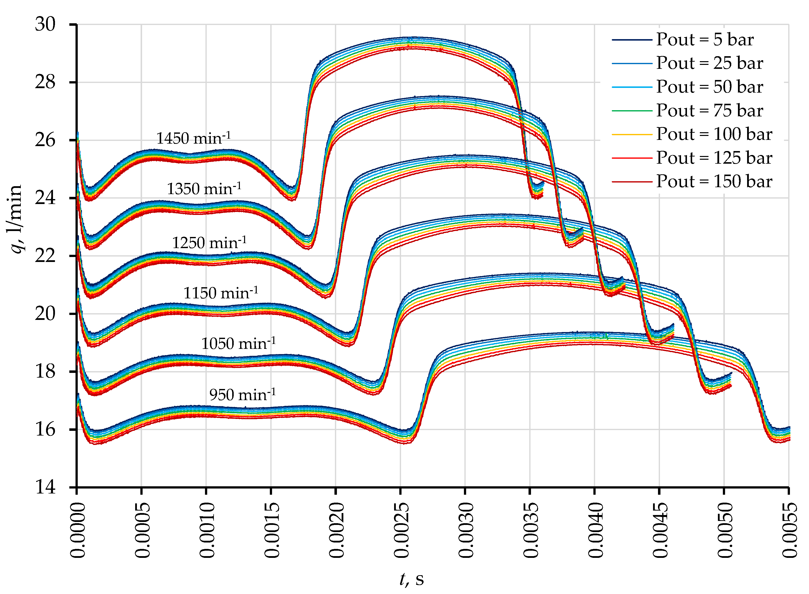
  Outlet: Set to “Pressure Outlet” type, with a pressure of 5, 25, 50, 75, 100, 125, or 150 bar, normal to the boundary;

  -

  Interface: Two contact regions are defined, Inlet Zone/Work Zone and Work Zone/Outlet Zone;

  -

  Internal: The three fluid regions mentioned above are defined;

  -

  Wall: The contours of all walls involved in the model are defined. There are a total of five groups: inlet walls, outlet walls, moving walls of the two gears, and work zone walls;

  -

  Mesh interfaces: The already mentioned two contact regions: Inlet Zone/Work Zone and Work Zone/Outlet Zone;

  -

  Dynamic mesh: In addition to the already-described settings, the dynamic mesh zones’ centers of rotation, as well as their rotational frequency through the User-Defined Function (UDF), are defined;

  -

  Solution Methods: Gradient—cell-based least squares; pressure—second order; momentum, turbulent kinetic energy, and turbulent dissipation rate—second order upwind;

  -

  Solution controls: Default values, except for absolute convergence criteria, which have been reduced from 1e-03 to 1e-06. This criterion is not met for 20 iterations; thus, the step never ends before all 20 iterations have been completed;

  -

  Time step size: For the purpose of the present study, the time step size is of the order of 2e-06 s, varying from 1e-06 to 3e-06, depending on the rotational frequency, as well as the stability of the solution.

• Initial condition at $t\le 0\therefore \overrightarrow{V}=0$;

• Velocity boundary condition on the casing wall: $\overrightarrow{V}=0$.

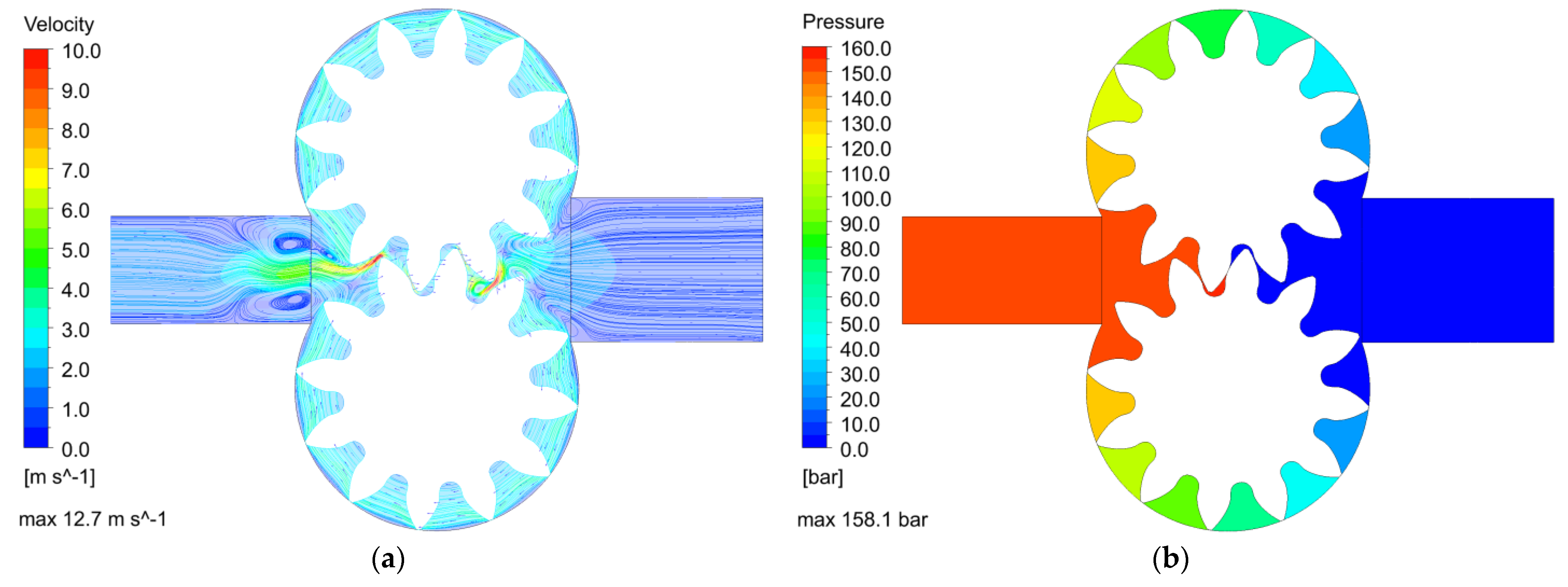
3. Numerical Results

Initially, a simulation was realized for a gear rotation angle of 125° at the nominal operating mode (n = 1450 min⁻¹, Δp = 150 bar). The resulting flow rate is presented in Figure 7.

The average value of the flow rate is 26.64 L/min and corresponds well to the actual measured value of 26.49 L/min. There is a periodicity in the flow ripple with a period of 30°, which corresponds to one tooth and one gap in gears with twelve teeth. It was, therefore, decided to limit the rotation angle to 30° in further simulations.

The observed flow ripple (23.7–29.1 L/min) is very large. Although it fully matches that published by other authors [52], it is still unrealistic. The explanation lies in the presence of discharge channels, which do not allow a large amount of fluid to be transferred from the high-pressure area to the low-pressure area. The influence of these channels is not accounted for in the current model, leading to the flow ripple shown. The effect is better illustrated in Figure 8 and is related to the number and position of the contact (meshing) points.

After specifying all the model parameters and the simulated rotation angle, forty-two simulations were carried out at six frequency modes (950, 1050, 1150, 1250, 1350, 1450) min⁻¹ and at seven load modes (5, 25, 50, 75, 100, 125, and 150) bar. Figure 9 shows the characteristics q(t) typical of a simulation of a gear pump with a simplified 2D model. From the depicted results, the average value of the flow rate can be determined, which can then be compared with experimentally measured values.

Figure 10a,b show the velocity distribution and the pressure distribution. A single-point contact gear position (also shown in Figure 8) was chosen, where the absence of discharge channels had the least effect on fluid movement between the teeth. It can be assumed that the simulation refers to the plane of symmetry, which is maximally distant from the discharge channels, and their influence on the velocity is not great. In the pressure distribution, however, the distortion due to the absence of these channels is substantial.

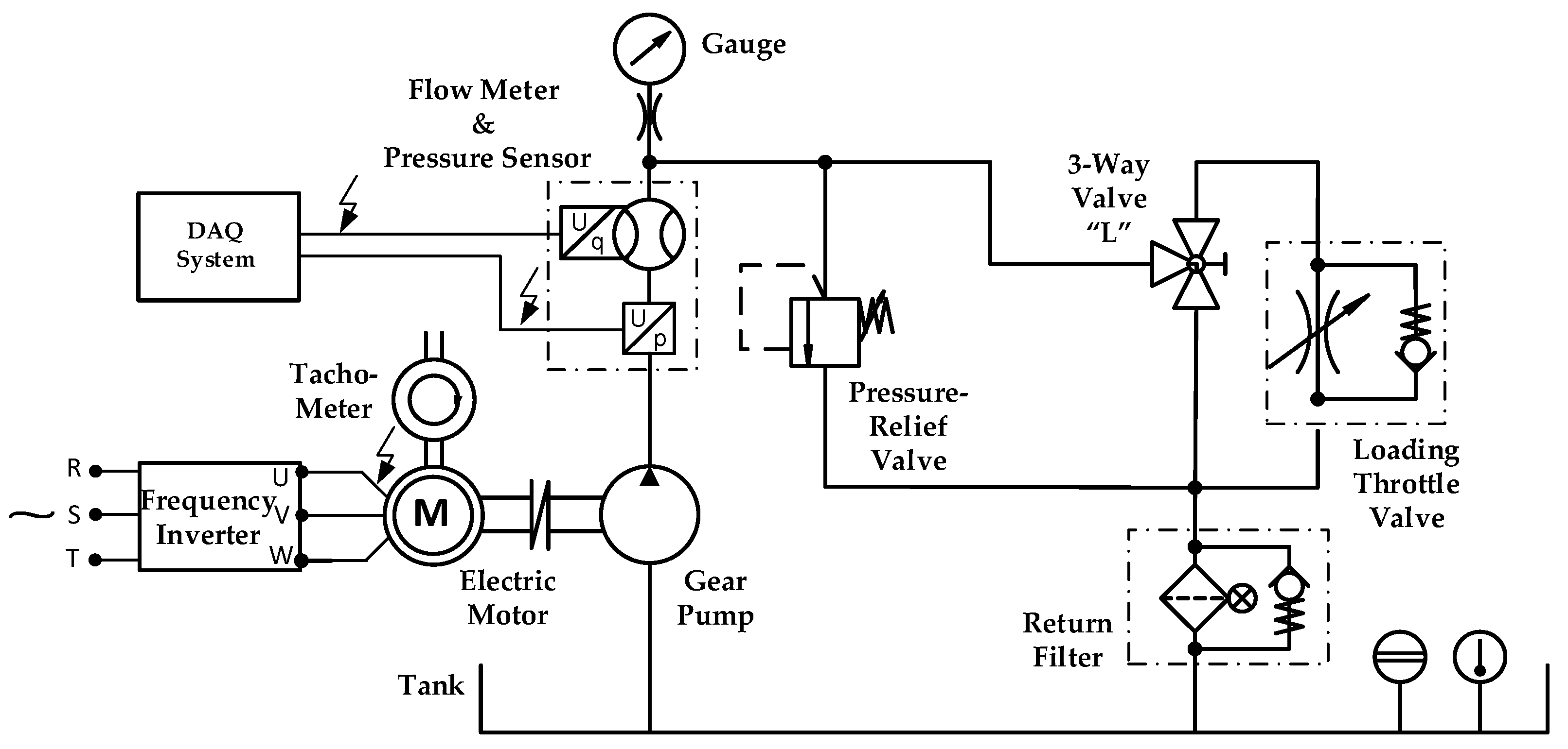
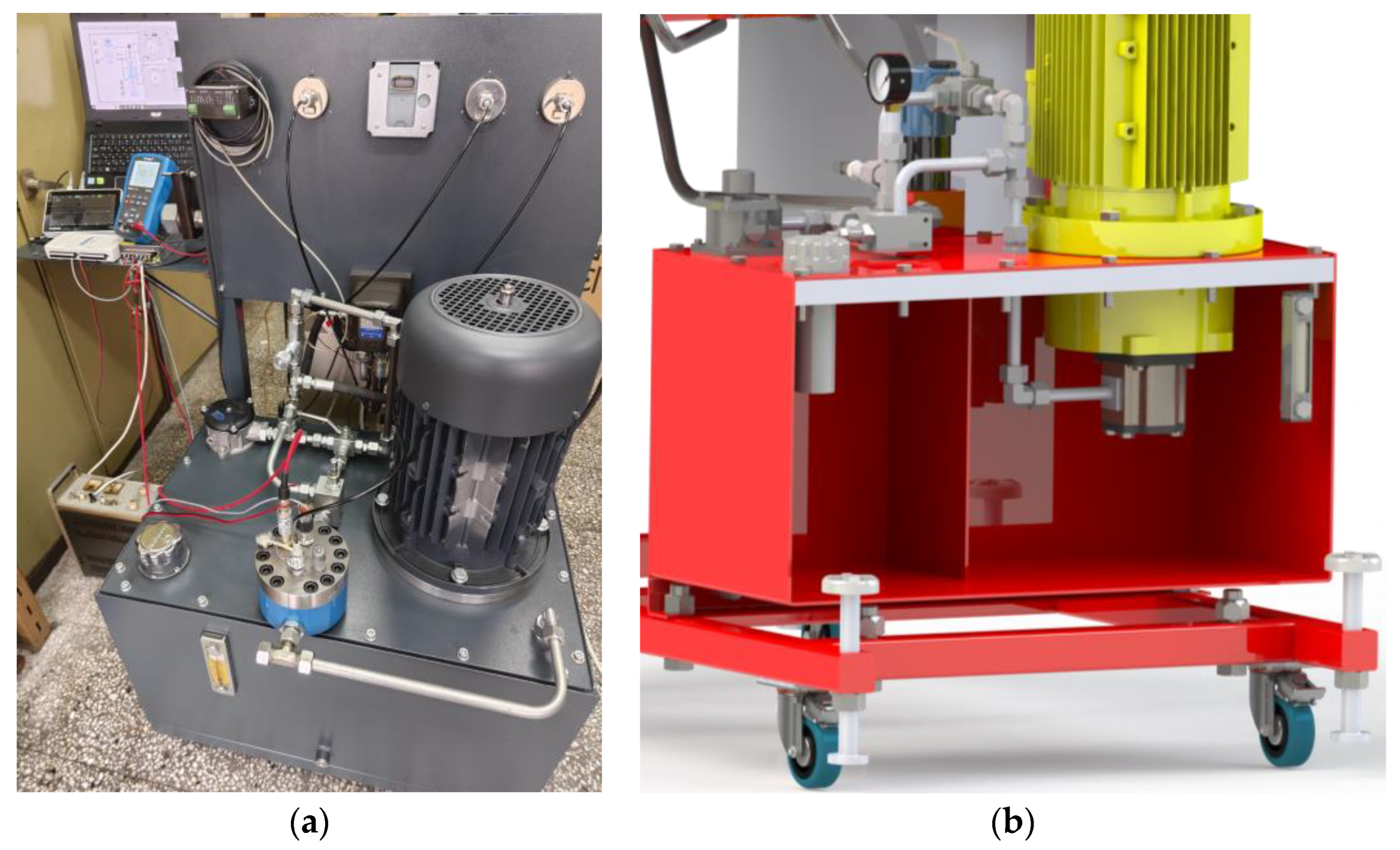
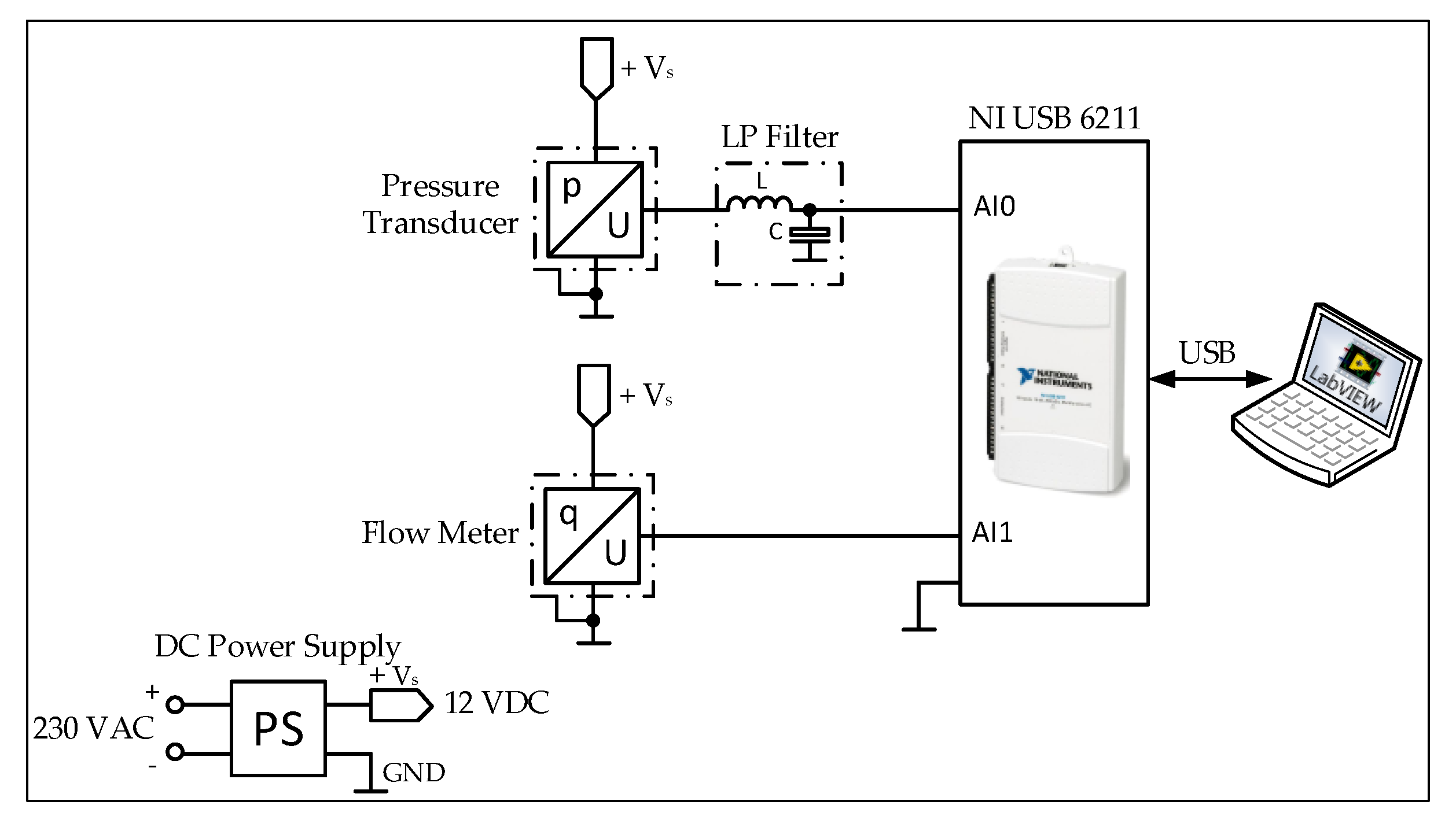
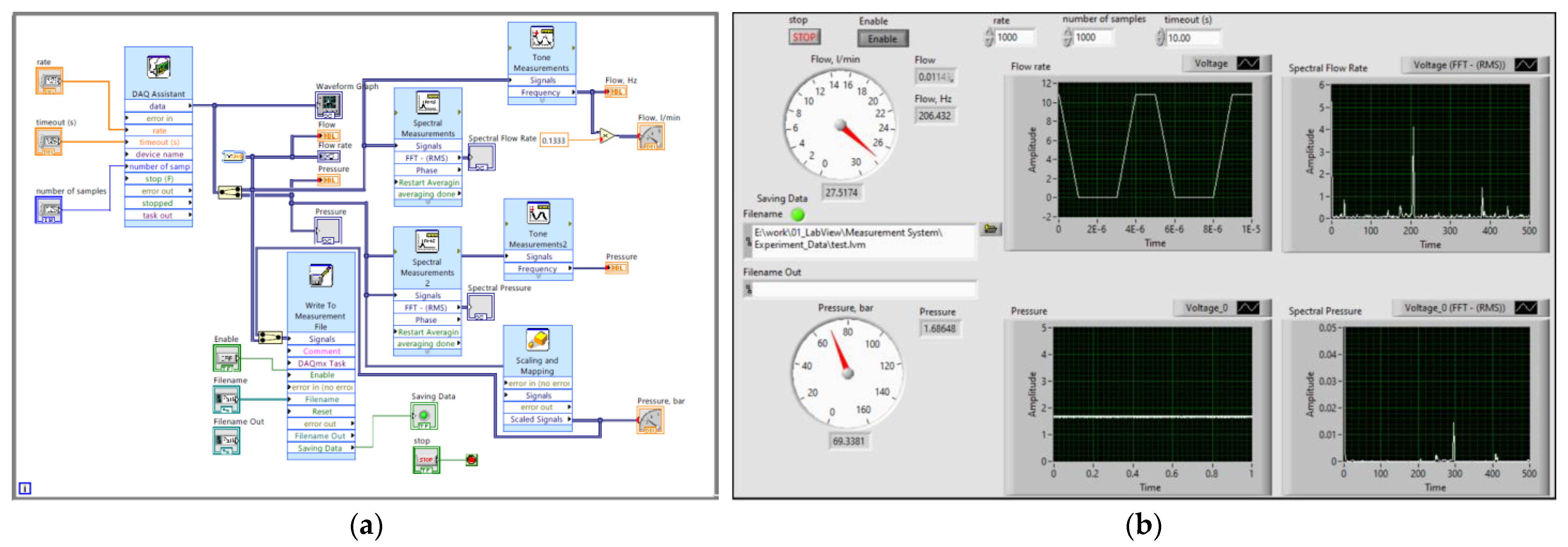
4. Experimental System Layout

For the purpose of validating the simulation results, the authors have developed a laboratory experimental setup. Its schematic is shown in Figure 11.

It is a modified version of an existing test bench and consists of two subsystems: hydraulic and DAQ. The hydraulic subsystem consists of a tank with a volume of 120 L, a motor pump group, and control-regulating hydraulic equipment, which performs the function of a loading system of the pump. The examined pump is driven by a three-phase asynchronous electric motor with a power of 7.5 kW. It is equipped with a frequency inverter allowing us to change the rotational frequency. A QG 100-type gear flow meter equipped with a frequency counter type HySense RS300 is connected to the pump discharge pipeline. A pressure transducer type MBS 1250 is connected to the flow meter. In this way, the flow meter provides the ability to measure flow rate and pressure signals at the same point of the pump’s discharge pipeline in different operating modes. From the point of view of an easy set of pressure values in different loading modes, the connection of the pressure transducer is duplicated by a gauge with a 0.6 accuracy class. After the flow meter, the directly operated pressure relief valve is connected in parallel with the pump. It serves to set the maximum value of the pressure in the system and determines the maximum permissible load of the pump. A throttle check valve is connected in parallel with the pressure relief valve. The throttle valve provides precise pressure adjustment within the range determined by the relief valve setting. In addition, a three-way “L”-type valve with manual control is connected between the throttle and pressure relief valve. The main position of the valve connects the pump discharge line directly to the tank, and the other position connects it to the loading system. In this way, switching between loading or non-loading mode is performed. In the return line, a return filter group is connected, which has a sufficient nominal flow rate to prevent additional pressure load. The parameters of the components used are presented in

Table 1. System components.

Component	Model	Parameters
Tank	Custom design	V = 120 L
Electric Motor	Miksan 134 M4	PEM = 7.5 kW n = 1500 min−1
External Gear Pump	-	Vp = 19 cm3
Direct Operated Pressure Relief Valve	CPL40/12	qmax = 40 L/min ∆pmax = 25 MPa
Throttle Check Valve	VRFU9003	qmax = 50 L/min ∆pmax = 35 MPa
3-Way Ball “L”-type Valve	GB3VH	qmax = 50 L/min ∆pmax = 35 MPa
Return Filter Group	MPF1002AG3P25NBP01	qmax = 50 L/min ƞ = 25 µm
Frequency Inverter	HNC HV 100	U = 380 V P = 7.5 kW
Flow Meter	QG 100 HySense RS 300	Gear type q = 0.7–70 L/min ∆pmax = 42 MPa
Pressure Transducer	MBS1250	∆p = 0–25 MPa Uout = 0.5–4.5 V
DAQ Device	NI USB 6211	8 Diff. or 16 SE ADC: 16 bits 250 kS/s
DC Power Supply	TEC 88	Uin = 230 VAC Uout = 0.5–12 VDC I = 0–2 A
Low Pass Filter	Custom design	R = 100 kΩ L = 100 μH C = 4.7 μF
Digital Tachometer (Laser)	DT2234A	nmax = 100 000 min−1

.

The experimental system is shown in Figure 12. A classic installation of the pump immersed in the tank is provided. The external gear pump is coupled to the motor by a standard mounting flange with a clutch. The pump delivery port is connected to a pipeline that exits the tank through bulkhead coupling bite-type fitting. The control-regulating and -measuring hydraulic equipment are located on the tank cover. In order to reduce the pressure losses in the pipelines, a size 15 × 1.5 mm was used.

A developed schematic solution of the DAQ system is shown in Figure 13. The main components of the system are a 12 VDC power supply unit type TEC 88, two transducers for flow rate and pressure (installed in the flow meter housing), and the DAQ device. The two transducers convert the two physical quantities into a voltage at their output. The output signal of each is connected to a corresponding analog input (AI) of the DAQ type NI USB 6211.

The DAQ has its own power supply from the USB of the mobile workstation. At the workstation, measurement software was developed by block modelling in the DAQ-selective software environment LabVIEW^® 2010. In addition to performing the parameterization and setting of the ADC channels through the developed block diagram (Figure 14a), the user interface (Figure 14b) allows real-time monitoring of the scaled values of the parameters, and their recording is created. It is possible to change the sample rate, number of samples, timeout, etc.

The output signal of the pressure transducer is a voltage in the range of 0.5–4.5 V, corresponding to a pressure range of 0–250 bar. Its conversion takes place in the software environment based on a linear characteristic from the transducer manufacturer. In connection with incoming noise disturbances in the signal generated from the electric power system, frequency inverter of the electric motor, lighting, etc., a low-pass (LP) filter is developed. It has been implemented as an analog circuit connected between the sensor and DAQ. All grounds and housing terminals are connected at a common point. The connections in the system are made with shielded wires.

Since the flow meter is a gear type, its converter is a frequency counter (RS 300). The frequency counter output signal is in the form of voltage impulses that are fed to the other input AI1 of the DAQ. The signal is recorded as the dataset in tabular form. This necessitates its processing to convert into a flow rate with the dimension L/min. It is performed in a MATLAB^® R2009b environment with a specially created script file, where the dataset is imported and processed by a loop counter. The measured flow rate signal sample time is 1 s, and it is described as a counter:

$$q_j={\displaystyle \sum _{i=0}^{T_0/n}{N}_q(i)},$$

(17)

where q_j is the flow rate, N_q(i) is the single impulse of sensor signal, and j = 1, 2,… is the number of samples. Therefore, the scaled flow rate in L/min is:

$$q\left(k\right)=K_{flow}{q}_j{T}_0,$$

(18)

where K_flow = 0.1338 is the calibration constant of the flow meter, T₀ = 1 s is the experimentally determinate measurement sample time, and k = T₀, 2T₀, 3T₀,… is the discrete time.

The high logical level is:

$$N_q\left(i\right)=1 \mathrm{at} q\left(i\right)-q\left(i-1\right)>0.3$$

(19)

and the low logical level is:

$$N_q\left(i\right)=0\mathrm{at} q\left(i\right)-q\left(i-1\right)\le 0.3,$$

(20)

where 0.3 is the threshold.

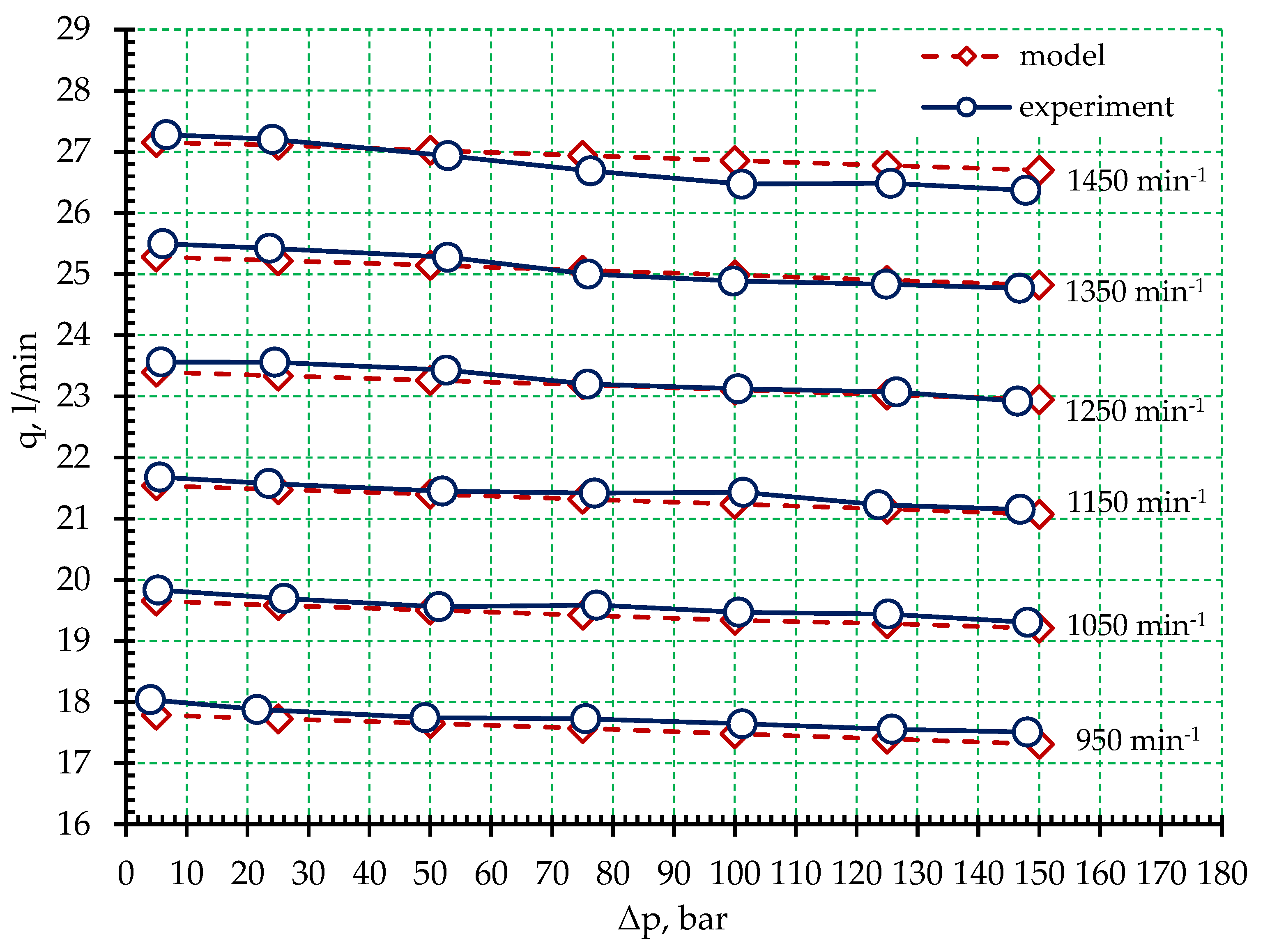
5. Validation of Numerical Results and Discussion

The developed 2D CFD model was validated by an experiment carried out on the developed laboratory setup. Figure 15 shows a comparison of the obtained q(Δp) characteristics from the CFD model and experiment for the considered pump operating modes.

Table 2. Experiment design and results.

Design		Results
nCFD min−1	ΔpCFD bar	qCFD,AVG L/min	nEXP min−1	qEXP,AVG, L/min	ΔpEXP,AVG bar	FIT %
950	5	17.79	951	18.04	4.04	93.38
	25	17.73	950	17.88	21.54
	50	17.65	949	17.75	49.14
	75	17.57	950	17.73	75.51
	100	17.48	953	17.64	101.23
	125	17.40	949	17.56	125.80
	150	17.31	952	17.51	148.06
1050	5	19.66	1048	19.83	5.29	95.44
	25	19.58	1049	19.69	25.98
	50	19.51	1048	19.56	51.39
	75	19.42	1050	19.59	77.32
	100	19.34	1051	19.47	100.66
	125	19.28	1053	19.44	125.21
	150	19.21	1048	19.31	148.11
1150	5	21.54	1147	21.68	5.58	96.58
	25	21.48	1148	21.57	23.49
	50	21.40	1148	21.45	51.97
	75	21.32	1152	21.42	76.97
	100	21.24	1154	21.43	101.38
	125	21.16	1149	21.23	123.62
	150	21.07	1145	21.15	146.89
1250	5	23.40	1248	23.56	5.79	97.21
	25	23.34	1254	23.56	24.46
	50	23.26	1256	23.43	52.60
	75	23.19	1248	23.20	75.86
	100	23.11	1246	23.12	100.54
	125	23.03	1251	23.07	126.57
	150	22.95	1246	22.92	146.45
1350	5	25.28	1348	25.50	6.08	96.72
	25	25.22	1352	25.42	23.62
	50	25.15	1353	25.28	52.86
	75	25.06	1348	25.00	75.91
	100	24.99	1353	24.89	99.75
	125	24.90	1348	24.84	124.87
	150	24.82	1349	24.77	146.79
1450	5	27.15	1447	27.28	6.67	94.10
	25	27.11	1448	27.20	24.07
	50	27.02	1447	26.94	52.88
	75	26.94	1446	26.69	76.31
	100	26.86	1444	26.47	101.14
	125	26.78	1450	26.49	125.59
	150	26.70	1450	26.37	147.81

presents the design and the results under different pump operating modes.

The results presented in Table 2 represent average values obtained from numerical and real experiments. The experimental and simulation results are analyzed by calculation of the average relative error (FIT). The FIT is expressed as a percentage:

$$FIT=100\left(1-{\displaystyle \sum _{i=1}^{N_i}\frac{\left|q_{EXP}-q_{CFD}\right|}{\left|q_{EXP}\right|}}\right),\%$$

(21)

where q_EXP is the experimentally obtained flow rate of the pump and q_CFD is the simulation flow rate obtained by the CFD model. The results for FIT are presented in Table 2.

The comparison (Figure 15) and level of FIT show a very good match between the model and experiment results. The small differences at rotational frequency 1450 min⁻¹ are due to a smooth increase in the temperature of the working fluid during the experiment, which is not accounted for by the CFD model.

The experiment was performed from minimum (950 min⁻¹) to maximum (1450 min⁻¹) rotation frequency. For each frequency mode, different pressure values are set from minimum (5 bar) to maximum (150 bar), which is maintained constantly by the loading system. The duration of the experiment and the variation of the parameters in the described sequence lead to heating of the working fluid, especially with an increase in the rotation frequency and pressure. In operating modes close to nominal (maximum frequency and high pressure), slight heating of the working fluid occurs, which is not accounted for in the simulation model and leads to the deviation visible in Figure 15 at 1450 min⁻¹. These temperature changes are not evaluated in the CFD model, and they are the cause for deviations in the match between simulation and experimental results (Figure 15).

Nevertheless, the equal negative slope of the model and experiment q(Δp) characteristics proves that the geometry of the pump is successfully reproduced, and the construction gaps are correctly specified. On the other hand, Figure 15 shows little or no difference between the model end experiment characteristics at all rotation frequency modes. This proves that the methodology for determining the gears’ face width is successful.

6. Conclusions

The main contribution of the article is the successful development of a simple 2D CFD model of the flow processes at an external gear pump. The simulation results were obtained in the form of characteristics presenting the flow rate as a function of the pressure q(Δp) and the flow rate as a function of the time q(t). These functions correspond to those published by other authors [23,26,33,40,52,53].

In contrast to a small part of the existing research [4,5,6,18,19,27,29,37,54,55], the numerical results are validated with the experiment [56]. For this purpose, an experimental setup was developed that successfully allowed us to measure the needed variables in all 42 operating modes of the experiment design. An analysis was carried out by comparing numerical and experimental results. Calculated FIT levels were in the range of 93–97%, which shows that a very good match was achieved. This proves the validity of the simplified 2D CFD model.

During the development of the CFD model, an original methodology was proposed to take into account the influence of the discharge channels on the displacement volume of the pump by adjusting the face width of the gears.

Detailed descriptions related to the implementation of the numerical model and the experimental setup are given, which may be useful for other researchers who choose the CFD approach. Particular attention is paid to the reverse fluid transfer that occurs in simple 2D CFD models, which has not been commented on by other authors.

For the developed CFD model, the accumulated knowledge and experience will serve to create more accurate and more complex models aimed at investigating vibrations and noise in the discharge pipeline caused by the operation of the pump in the hydraulic power unit.

References

1. Findeisen, D.; Helduser, S. Ölhydraulik; Springer: Berlin, Germany, 2015. [Google Scholar]
2. Ivantysyn, J.; Ivantysynova, M. Hydrostatic Pumps and Motors: Principles, Design, Performance, Modelling, Analysis, Control and Testing; Academia Books International: New Delhi, India, 2001. [Google Scholar]
3. Manring, N.D.; Kasaragadda, S.B. The theoretical flow ripple of an external gear pump. J. Dyn. Syst. Meas. Control. Trans. ASME 2003, 125, 396–404. [Google Scholar] [CrossRef]
4. Choudhuri, K.; Biswas, N.; Mandal, S.K.; Mitra, C.; Biswas, S. A numerical study of an external gear pump operating under different conditions. Mater. Today Proc. 2022, in press. [Google Scholar] [CrossRef]
5. Zhao, X.; Vacca, A.; Dhar, S. Numerical Modeling of a Helical External Gear Pump with Continuous-Contact Gear Profile: A Comparison between a Lumped-Parameter and a 3D CFD Approach of Simulation. In Proceedings of the BATH/ASME 2018 Symposium on Fluid Power and Motion Control FPMC2018, Bath, UK, 12–14 September 2018. [Google Scholar]
6. Orlandi, F.; Muzzioli, G.; Milani, M.; Paltrinieri, F.; Montorsi, L. Development of a numerical approach for the CFD simulation of a gear pump under actual operating conditions. Fluids 2023, 8, 244. [Google Scholar] [CrossRef]
7. Corvaglia, A.; Rundo, M.; Bonati, S.; Rigosi, M. Simulation and experimental activity for the evaluation of the filling capability in external gear pumps. Fluids 2023, 8, 251. [Google Scholar] [CrossRef]
8. Gafurov, S.; Rodionov, L.; Makaryants, G. Simulation of Gear Pump Noise Generation. In Proceedings of the 9th FPNI Ph.D. Symposium on Fluid Power FPNI 2016, Florianópolis, Brazil, 26–28 October 2016. [Google Scholar]
9. Tang, C.; Wang, Y.S.; Gao, J.H.; Guo, H. Fluid-sound coupling simulation and experimental validation for noise characteristics of a variable displacement external gear pump. Noise Control. Eng. J. 2014, 62, 123–131. [Google Scholar] [CrossRef]
10. Fiebig, W. Influence of the inter teeth volumes on the noise generation in external gear pumps. Arch. Acoust. 2014, 39, 261–266. [Google Scholar] [CrossRef]
11. Mucchi, E.; Rivola, A.; Dalpiaz, G. Modelling dynamic behaviour and noise generation in gear pumps: Procedure and validation. Appl. Acoust. 2014, 77, 99–111. [Google Scholar] [CrossRef]
12. Woo, S.; Opperwall, T.; Vacca, A.; Rigosi, M. Modeling noise sources and propagation in external gear pumps. Energies 2017, 10, 1068. [Google Scholar] [CrossRef]
13. Fiebig, W. Noise Control of Fluid Power Units. In Proceedings of the 23rd International Congress on Sound and Vibration: From Ancient to Modern Acoustics, Athens, Greece, 10–14 July 2016. [Google Scholar]
14. Carletti, E.; Pedrielli, F. Sound Power Levels of Hydraulic Pumps using Sound Intensity Techniques: Towards More Accurate Values? In Proceedings of the 12th International Congress on Sound and Vibration, Lisbon, Portuga, 11–14 July 2005. [Google Scholar]
15. Osiński, P.; Deptuła, A.; Deptuła, A.M. Analysis of the Gear Pump’s Acoustic Properties Taking into Account the Classification of Induction Trees. Energies 2023, 16, 4460. [Google Scholar] [CrossRef]
16. ISO 16902-1:2003; Hydraulic Fluid Power—Test Code for the Determination of Sound Power Levels of Pumps Using Sound Intensity Techniques: Engineering Method—Part 1: Pumps. ISO: Geneva, Switzerland, 2003.
17. Mitov, A.; Nedelchev, K.; Kralov, I. Experimental Study of Sound Pressure Level in Hydraulic Power Unit with External Gear Pump. Processes 2023, 11, 2399. [Google Scholar] [CrossRef]
18. Stan, L.C.; Gordes, A.N.; Agape, A.G. Numerical simulation of a gear pump. Int. J. Mod. Manuf. Technol. 2023, 15, 107–114. [Google Scholar]
19. Patil, S. Numerical Simulation of Multi-Dimensional Flows in a Gear Pump. Master’s Thesis, Youngstown State University, Youngstown, OH, USA, 2006. [Google Scholar]
20. Maccioni, L.; Concli, F. Computational fluid dynamics applied to lubricated mechanical components: Review of the approaches to simulate gears, bearings, and pumps. Appl. Sci. 2020, 10, 1–29. [Google Scholar] [CrossRef]
21. Mali, P.S.; Joshi, G.S.; Patil, I.A. Performance improvement of external gear pump through CFD analysis. Int. Res. J. Eng. Technol. 2018, 5, 430–433. [Google Scholar]
22. Del Campo, D. Analysis of the Suction Chamber of External Gear Pumps and Their Influence on Cavitation and Volumetric Efficiency. Ph.D. Thesis, Universitat Politècnica de Catalunya, Barcelona, Spain, 2012. [Google Scholar]
23. Munih, J.; Hočevar, M.; Petrič, K.; Dular, M. Development of CFD-based procedure for 3D gear pump analysis. Eng. Appl. Comput. Fluid Mech. 2020, 14, 1023–1034. [Google Scholar] [CrossRef]
24. Yoon, Y.; Park, B.-H.; Shim, J.; Han, Y.-O.; Hong, B.-J.; Yun, S.-H. Numerical simulation of three-dimensional external gear pump using immersed solid method. Appl. Therm. Eng. 2017, 118, 539–550. [Google Scholar] [CrossRef]
25. Corvaglia, A.; Ferrari, A.; Rundo, M.; Vento, O. Three-dimensional model of an external gear pump with an experimental evaluation of the flow ripple. Proc. Inst. Mech. Eng. Part C J. Mech. Eng. Sci. 2021, 235, 1097–1105. [Google Scholar] [CrossRef]
26. Frosina, E.; Senatore, A.; Rigosi, M. Study of a high-pressure external gear pump with a computational fluid dynamic modeling approach. Energies 2017, 10, 1113. [Google Scholar] [CrossRef]
27. Močilan, M.; Husár, Š.; Labaj, J.; Žmindák, M. Non-Stationary CFD Simulation of a Gear Pump. In Proceedings of the 21st International Polish-Slovak Conference “Machine Modeling and Simulations 2016”, Hucisko, Poland, 8–11 September 2017. [Google Scholar]
28. Jędraszczyk, P.; Fiebig, W. CFD model of an external gear pump. In RESRB 2016: Proceedings of the 13th International Scientific Conference, Wrocław, Poland, 22–24 June 2016; Springer: Berlin, Germany, 2017; pp. 221–231. [Google Scholar]
29. Castilla, R.; Gamez-Montero, P.J.; Del Campo, D.; Raush, G.; Garcia-Vilchez, M.; Codina, E. Three-dimensional numerical simulation of an external gear pump with decompression slot and meshing contact point. J. Fluids Eng. Trans. ASME 2015, 137, 041105. [Google Scholar] [CrossRef]
30. Mhana, W.; Popov, G. Method for Investigation of the Pressure Variation in the Chambers of Gear Pumps with Symmetric and Asymmetric Tooth Profiles Used in Electrohydraulic Drive Systems. In Proceedings of the 16th Conference on Electrical Machines, Drives and Power Systems, Varna, Bulgaria, 6–8 June 2019. [Google Scholar]
31. Corvaglia, A.; Rundo, M.; Casoli, P.; Lettini, A. Evaluation of tooth space pressure and incomplete filling in external gear pumps by means of three-dimensional CFD simulations. Energies 2021, 14, 342. [Google Scholar] [CrossRef]
32. Ouyang, T.; Mo, X.; Lu, Y.; Wang, J. CFD-vibration coupled model for predicting cavitation in gear transmissions. Int. J. Mech. Sci. 2022, 225, 107377. [Google Scholar] [CrossRef]
33. Killedar, J.S. CFD Analysis of Gear Pump. Master’s Thesis, Youngstown State University, Youngstown, OH, USA, 2005. [Google Scholar]
34. Heisler, A.S.; Moskwa, J.J.; Fronczak, F.J. Simulated Helical Gear Pump Analysis using a New CFD Approach. In Proceedings of the ASME Fluids Engineering Division Summer Conference FEDSM2009, Vail, CO, USA, 2–6 August 2009. [Google Scholar]
35. Labaj, J.; Husar, S. Analysis of Gear Pump Designed for Manufacturing Processes. Appl. Mech. Mater. 2015, 803, 163–172. [Google Scholar] [CrossRef]
36. Lee, J.-H.; Lee, S.-W. Numerical Simulations of Cavitation Flow in Volumetric Gear Pump. J. Korean Soc. Vis. 2011, 9, 28–34. [Google Scholar]
37. Del Campo, D.; Castilla, R.; Raush, G.A.; Gamez Montero, P.J.; Codina, E. Numerical analysis of external gear pumps including cavitation. J. Fluids Eng. Trans. ASME 2012, 134, 081105. [Google Scholar] [CrossRef]
38. Strasser, W. CFD Investigation of Gear Pump Mixing. In Proceedings of the ASME International Mechanical Engineering Congress and Exposition, Orlando, FL, USA, 5–11 November 2005. [Google Scholar]
39. Strasser, W. CFD investigation of gear pump mixing using deforming/agglomerating mesh. J. Fluids Eng. Trans. ASME 2007, 129, 476–484. [Google Scholar] [CrossRef]
40. Ghazanfarian, J.; Ghanbari, D. Computational fluid dynamics investigation of turbulent flow inside a rotary double external gear pump. J. Fluids Eng. Trans. ASME 2015, 137, 021101. [Google Scholar] [CrossRef]
41. Qi, F.; Dhar, S.; Nichani, V.H.; Srinivasan, C.; Wang, D.M.; Yang, L.; Bing, Z.; Yang, J.J. A CFD study of an Electronic Hydraulic Power Steering Helical External Gear Pump: Model Development, Validation and Application. SAE Int. J. Passeng. Cars—Mech. Syst. 2016, 9, 346–352. [Google Scholar] [CrossRef]
42. Martínez, J. Mesh Handling for the CFD Simulation of External Gear Pumps. In Positive Displacement Machines: Modern Design Innovations and Tools, 1st ed.; Sultan, I., Phung, T., Eds.; Elsevier: Amsterdam, The Netherlands, 2019; pp. 345–368. [Google Scholar]
43. Ull, A.R. Study of Mesh Deformation Features of an Open Source CFD Package and Application to a Gear Pump Simulation; Enginyeria Aeronàutica, Universitat Politècnica De Catalunya: Barcelona, Spain, 2012. [Google Scholar]
44. Mucchi, E.; Dalpiaz, G.; Rivola, A. Dynamic behavior of gear pumps: Effect of variations in operational and design parameters. Meccanica 2011, 46, 1191–1212. [Google Scholar] [CrossRef]
45. Marinaro, G.; Frosina, E.; Senatore, A. A Numerical Analysis of an Innovative Flow Ripple Reduction Method for External Gear Pumps. Energies 2021, 14, 471. [Google Scholar] [CrossRef]
46. Mott, R. Machine Elements in Mechanical Design; Prentice Hall: Hoboken, NJ, USA, 2004. [Google Scholar]
47. Will, D.; Ströhl, H. Einführung in die Hydraulik und Pneumatik; VEB Verlag Technik: Berlin, Germany, 1983. [Google Scholar]
48. Findeisen, F.; Findeisen, D. Ölhydraulik in Theorie und Anwendung; Schweizer Verlag Haus: Zürich, Switzerland, 1968. [Google Scholar]
49. Angelov, I. Hydraulic Transmissions; TU-Sofia: Sofia, Bulgaria, 2015. [Google Scholar]
50. Bashta, T.M. Engineering Hydraulics: Handbook; Mashinostroenie: Moscow, Russia, 1963. [Google Scholar]
51. Cengel, Y.A.; Cimbala, J.M. Fluid Mechanics: Fundamental and Applications; McGraw-Hill: New York, NY, USA, 2013. [Google Scholar]
52. Szwemin, P.; Fiebig, W. The Influence of Radial and Axial Gaps on Volumetric Efficiency of External Gear Pumps. Energies 2021, 14, 4468. [Google Scholar] [CrossRef]
53. Adake, D.G.; Dhote, N.D.; Khond, M.P. Experimentation and 2D Fluid Flow Simulation over an External Gear Pump. J. Phys. Conf. Ser. 2023, 2601, 012029. [Google Scholar] [CrossRef]
54. Zhou, W.; Yu, D.; Wang, Y.; Shi, J.; Gan, B. Research on the Fluid-Induced Excitation Characteristics of the Centrifugal Pump Considering the Compound Whirl Effect. Facta Univ. Ser. Mech. Eng. 2023, 21, 223. [Google Scholar] [CrossRef]
55. Bilalov, R.A.; Smetannikov, O.Y. Numerical Study of the Hydrodynamics of an External Gear Pump. J. Appl. Mech. Tech. Phys. 2022, 63, 1284–1293. [Google Scholar] [CrossRef]
56. Li, X.; Zhang, L.; Zhang, Y. Numerical Study on the Influence of Different Operating Conditions on Mixing Uniformity of the Helical Gear Pump Mixer. Processes 2023, 11, 3223. [Google Scholar] [CrossRef]
Figure 1. Spur gear terminology.
Processes 12 00261 g001
Figure 2. Created tooth profile of the spur gears: (a) imposition of sketches on the captured images; (b) comparison of the resulting tooth profile with high-resolution photographs.
Processes 12 00261 g002
Figure 3. A 3D disassembled state model of the external gear pump.
Processes 12 00261 g003
Figure 4. Simplification of the fluid body: (a) initial 3D fluid body; (b) simple 2D model with its three zones.
Processes 12 00261 g004
Figure 5. Discharge channel influence: (a) fluid transfer in case of omitting discharge channels in a simple 2D model; (b) discharge channels’ actual shape.
Processes 12 00261 g005
Figure 6. Finite element mesh view and parameters: (a) start (input) mesh; (b) final (remeshed) mesh at 30° rotation.
Processes 12 00261 g006
Figure 7. Flow rate at the nominal operating mode (2D CFD model result).
Processes 12 00261 g007
Figure 8. Flow ripple in the dependence of the teeth position.
Processes 12 00261 g008
Figure 9. Simulation results for the flow rate of the pump at different operating modes.
Processes 12 00261 g009
Figure 10. Distributions: (a) velocity; (b) pressure.
Processes 12 00261 g010
Figure 11. Hydraulic circuit diagram of the experimental setup.
Processes 12 00261 g011
Figure 12. Experimental setup: (a) photograph; (b) hydraulic power unit setup (3D CAD model).
Processes 12 00261 g012
Figure 13. DAQ system basic scheme.
Processes 12 00261 g013
Figure 14. LabVIEW DAQ system-developed software: (a) block scheme; (b) user interface.
Processes 12 00261 g014
Figure 15. Comparison between average flow rates obtained by the CFD model and the experiment.
Processes 12 00261 g015