Development of a Fleet Management System for Multiple Robots’ Task Allocation Using Deep Reinforcement Learning

Abstract

This paper presents a fleet management system (FMS) for multiple robots, utilizing deep reinforcement learning (DRL) for dynamic task allocation and path planning. The proposed approach enables robots to autonomously optimize task execution, selecting the shortest and safest paths to target points. A deep Q-network (DQN)-based algorithm evaluates path efficiency and safety in complex environments, dynamically selecting the optimal robot to complete each task. Simulation results in a Gazebo environment demonstrate that Robot 2 achieved a path 20% shorter than other robots while successfully completing its task. Training results reveal that Robot 1 reduced its cost by 50% within the first 50 steps and stabilized near-optimal performance after 1000 steps, Robot 2 converged after 4000 steps with minor fluctuations, and Robot 3 exhibited steep cost reduction, converging after 10,000 steps. The FMS architecture includes a browser-based interface, Node.js server, rosbridge server, and ROS for robot control, providing intuitive monitoring and task assignment capabilities. This research demonstrates the system’s effectiveness in multi-robot coordination, task allocation, and adaptability to dynamic environments, contributing significantly to the field of robotics.

1. Introduction

With the rapid development of automation technology, multi-robot systems (MRS) have been widely used in various fields, such as industrial automation [1], warehousing logistics [2,3], rescue operations [4,5], and exploration missions [6,7]. Multi-robot systems can significantly improve efficiency and accuracy by collaborating to execute complex tasks. However, as the complexity of tasks and the number of robots increase, effectively managing and allocating tasks, ensuring efficient task execution, and maintaining system security have become major challenges in current research. Particularly in dynamic and uncertain environments, how to coordinate cooperation and competition among robots and optimize task allocation strategies has become a key issue in the study of multi-robot systems. Especially in dynamic and uncertain environments, how to coordinate cooperation among robots and optimize task allocation strategies has become a key issue in the study of multi-robot systems [8,9]. For example, autonomous underwater vehicles (AUVs) operate under constrained bandwidth and unreliable communication, making coordination and mutual control particularly challenging. This highlights the need for robust, decentralized task allocation approaches that can adapt to harsh and dynamic conditions.

Most existing multi-robot systems rely on centralized control or pre-defined path planning methods, making them less adaptable to rapidly changing environments and flexible task allocation. These limitations are especially evident in industrial and harsh environments, where communication and cooperation are difficult. To address this issue, this paper proposes a multi-robot fleet management system based on reinforcement learning (RL) and path planning. The system not only coordinates multiple robots to complete different tasks but also learns and optimizes to automatically decide which robot should execute each task, ensuring both the shortest and safest paths are selected. By integrating dynamic decision-making and robust optimization, the proposed method offers potential applications in harsh environments such as AUV coordination, where reliable communication is limited, similar to the scenarios studied by [10]. This adaptability makes the system suitable for a broad range of applications, from industrial automation to complex, communication-constrained scenarios.

A fleet management system for multiple robots [11,12] is essential for ensuring efficient, scalable, and safe operations in any application where robots are used in significant numbers. It brings together the coordination, control, and optimization needed to manage a complex and dynamic fleet effectively [13,14,15]. In a multi-robot environment, a fleet management system helps in efficiently assigning tasks to different robots based on their current state, location, and capabilities. This ensures that tasks are completed in the shortest time possible and resources are used optimally. A well-designed fleet management system enables better coordination among robots. It allows them to work together seamlessly, avoiding conflicts such as collisions or duplication of tasks. Fleet management systems provide real-time monitoring capabilities, allowing operators to track the status, location, and performance of each robot. This enables quick decision-making in response to any issues, such as a robot failure or unexpected obstacles, ensuring minimal disruption to operations. The fleet management system can collect data from multiple robots, which can be analyzed to improve future operations.

In the research and development of multi-robot fleet management systems, several critical areas are explored to enhance the efficiency, coordination, and robustness of such systems. The main research focuses include task allocation and scheduling [16], where algorithms are developed to distribute tasks among robots efficiently, ensuring optimal completion within time and resource constraints. Path planning and obstacle avoidance [17] are also essential, requiring the development of algorithms that enable robots to navigate shared spaces autonomously while avoiding collisions, especially in dynamic environments. Furthermore, collaborative control strategies [18] are explored to improve system performance through distributed control, enabling synchronized movements and shared tasks among robots. In communication and networking [19], efficient wireless communication protocols are important for real-time data transmission, while distributed network architectures enhance system scalability and robustness.

In multi-robot systems, reinforcement learning (RL) [20,21,22,23,24] can be effectively used to achieve autonomous task allocation and path planning. By utilizing RL algorithms, robots can learn how to optimally allocate tasks and plan the shortest or safest paths within a given environment. This is particularly useful in complex task scenarios, such as automated sorting and delivery in logistics warehouses, where robots need to rapidly and efficiently complete tasks in a dynamic environment. RL algorithms are capable of adapting to changes in the environment, continuously optimizing paths and task distribution, thereby ensuring overall system efficiency. Reinforcement learning (RL) can assist multiple robots in achieving coordinated navigation within shared spaces while also avoiding collisions. Through learning, robots can develop a collaborative mechanism that allows them to complete their respective tasks without interfering with each other. For example, in a factory or a warehouse, multiple automated guided vehicles (AGVs) may need to move simultaneously through narrow corridors while transporting goods. RL algorithms can enable these vehicles to intelligently avoid obstacles and optimize their movement paths, thereby reducing traffic congestion and minimizing the risk of collisions. To apply reinforcement learning (RL) to multi-robot path planning, several key steps need to be followed. These steps include environment modeling, algorithm selection and implementation, training and testing, and finally deployment and optimization. In the multi-robot systems, the state space represents the pose, velocity, and the positions of obstacles within the environment for each robot. The state space is often a combination of these variables, which allows each robot to understand not only its own state but also how its actions may impact the states of other robots. A reward function is critical because it determines the feedback that the robots receive after executing actions. If the robot avoids obstacles, reaches target points, or chooses the shortest path, a positive reward will be given. Otherwise, a negative reward will be given. Deep Q-networks (DQN) [25,26] or policy gradient methods [27] are the RL algorithms, which help in learning the policies that guide the robots’ actions based on their states. Before deploying the RL model in the real world, extensive training in simulated environments is necessary. This allows the robots to explore a wide variety of scenarios and learn the best strategies without the risks associated with real-world testing. Once the model is trained, it needs to be tested both in simulation and in real-world environments. If successful in testing, the model can be deployed in real-world applications. This paper proposes a DRL based on DQN to help multiple robots find the shortest and safest paths. In the neural network architecture, the inputs are the robot’s position and the length of the path. The output is the action with the max Q value. A well-defined reward structure ensures that the robots can efficiently navigate to their goals while avoiding obstacles. If the robot collides with the obstacle, the reward value is −1 and the done value is True. If the robot moves into the obstacle-free space, the reward value is 0 and the done value is False. If the robot arrives at the goal point, the reward value is calculated based on the length of the path and the done value is True. By incorporating a prioritized experience replay mechanism, the algorithm ensures that the most informative samples are emphasized during training, enhancing prediction accuracy and learning efficiency. The use of an e-greedy strategy balances exploration and exploitation, gradually leading the robots to adopt optimal behaviors.

This paper develops a fleet management system to dynamically manage multiple robots. The browser sends HTTP POST/GET requests to the Node.js server for saving or loading navigation goals from the goals.json file. A graphical user interface (GUI) is designed for the real-time monitoring of robot statuses and control of their behaviors. The browser communicates with the rosbridge directly via WebSocket to send commands or subscribe to ROS topics to monitor robots’ status. The Node.js server executes backend scripts to ROS system by rosbridge WebSocket. Rosbridge translates the WebSocket message into ROS topics and allows communication between the browser (and Node.js) and the ROS system. The ROS system executes commands and publishes data by ROS topics. The ROS system employs reinforcement learning algorithms to enable each robot to find the shortest and safest path to its target point. Robots compare their respective paths to determine which one should execute a given task. The robot that finds the shortest path receives the highest positive reward, while those that fail to find a safe path are penalized. The system leverages reinforcement learning to dynamically optimize task allocation and path selection among the robots.

Compared to existing approaches, the proposed method provides significant advantages in dynamic and real-time multi-robot task allocation. Ref. [28] introduced a multi-objective evolutionary algorithm combined with DRL, focusing on optimizing complex task scenarios but with higher computational costs, making it less suited for real-time applications. Ref. [29] proposed a two-stage reinforcement learning approach that incorporates a pre-allocation strategy and attention mechanisms, offering flexibility for task generalization but increasing system complexity and computation time. In contrast, the proposed method leverages a deep Q-network (DQN) with prioritized experience replay to dynamically allocate tasks and optimize paths based on safety and efficiency, achieving real-time decision-making. Furthermore, by integrating map segmentation and robot grouping strategies, the system scales effectively to larger fleets while ensuring high navigation success rates and collision-free operation in dynamic environments.

This paper makes the following contributions to the integration of DRL and FMS in multi-robot systems. (1) DRL for task allocation and path planning: DRL is applied to dynamically allocate tasks and optimize path selection, ensuring adaptability to changing environments. The system prioritizes safety and efficiency, dynamically optimizing task distribution and path decisions. (2) Integration of RL into fleet management systems: The proposed FMS utilizes DRL to compare paths and assign tasks dynamically, with robots receiving rewards for efficient task completion and safe navigation. Robots collaborate seamlessly, avoiding conflicts and improving overall performance in shared environments. (3) Web-based monitoring and control: A browser-based GUI enables monitoring of robot statuses and task execution. Communication between the GUI, Node.js server, and ROS system is achieved using HTTP POST/GET requests and WebSocket protocols by rosbridge. (4) Practical implementation and testing: The system is trained in simulated environments to explore complex scenarios without risks. By integrating RL with FMS, the proposed system addresses critical challenges in dynamic task allocation and path planning for multi-robot systems, offering a scalable, adaptable, and efficient solution for complex robotic operations.

2. Reinforcement Learning Algorithm for Multiple Mobile Robots Task Allocation

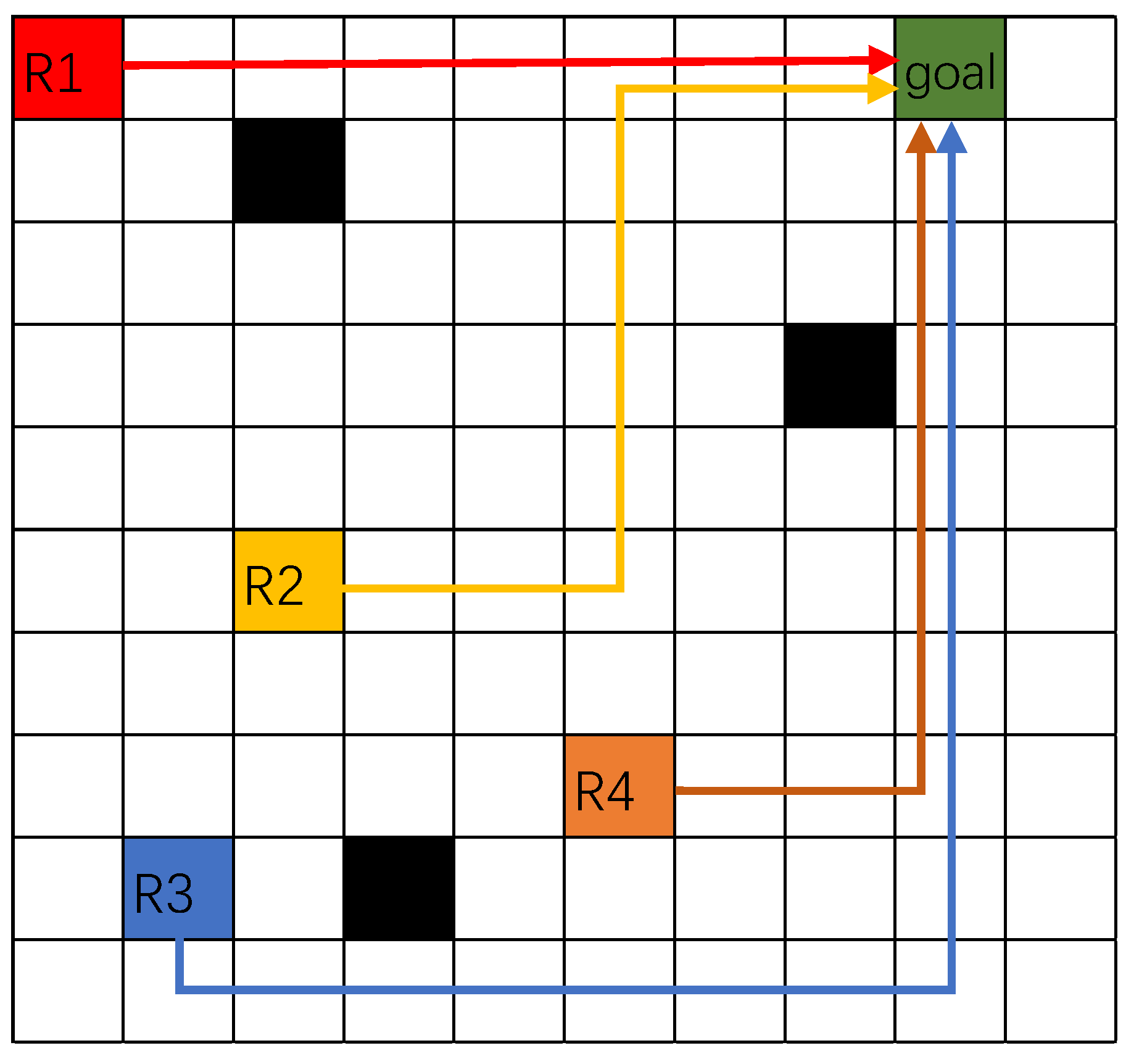
A deep reinforcement learning (DRL) algorithm is utilized in the multi-robot system to efficiently allocate tasks. As shown in Figure 1, within obstacles in the environment, a single goal point is assigned to the system, and several robots can move toward this goal. However, only one robot is selected to complete the task, and the chosen robot has the shortest and safest path to the goal. The DRL algorithm allows the system to learn and optimize task allocation by continuously evaluating the robots’ paths and selecting the most suitable robot based on safety and efficiency. In Figure 1, the green represents the goal point, which is the target location for the robots. There are four robots (R1, R2, R3, and R4) in the environment, each represented by different colored blocks: red, yellow, blue, and brown, respectively. The black blocks in the environment are obstacles that the robots must avoid when navigating toward the goal point. After training and testing the DRL algorithm, it is determined that R1 can safely navigate to the goal point along the shortest path, so R1 is selected and assigned the task of moving to the goal point, completing the mission efficiently. When applying the DRL algorithm, the system sets each robot’s starting point as an obstacle to prevent collisions between robots. This ensures that other robots do not select these points as feasible paths during route planning, fundamentally avoiding initial stage path conflicts. Using the DRL algorithm, each robot independently plans the shortest and safest path from its starting point to the target point. The system then compares all planned paths and selects the robot with the shortest path to execute the task and move to the target point. During this process, the other robots remain stationary, waiting for the task to be completed. This approach combines dynamic path planning with a static waiting mechanism, reducing the complexity of path planning while effectively preventing collisions during task execution. It ensures the efficiency and safety of task allocation and execution in the multi-robot system.

In each episode of the DRL algorithm, the observation is initialized first, which includes defining the state of each robot $s_i$ and the length of the path $l_i$. $i$ is the number of the robot. The state of each robot $s_i$ is represented by its coordinates $\left[x_i,y_i\right]$, which indicate the robot’s position in the environment. $l_i$ is defined as zero. At the beginning of the episode, the start points and goal point are assigned to each robot. In the loop, the observation is put into the neural network as the input. Generate a random number $n_r$. If $n_r$ is smaller than e-greedy, an action $a_i^t$ is chosen within the max Q value. Otherwise, the random action $a_i^t$ is selected. There are four actions for each robot, such as moving forward, moving backward, turning to left, and turning to right. Execute the action on each robot. The outputs include the observation, reward, and done. The observation consists of the robot state $\left[x_i^{t+1},y_i^{t+1}\right]$ and the robot moving step’s path length from the start point $l_i^t$. If the robot collides with the obstacle, the reward value is −1, and the done value is True. If the robot moves into the obstacle-free space, the reward value is 0, and the done value is False. If the robot arrives at the goal point, the reward value $r_i$ is calculated as (1), and the done value is True. Because the start point and the goal point are not the same points, the robot’s moving step path length is not zero.

$$r_i=100/l_i^{t+1}$$

(1)

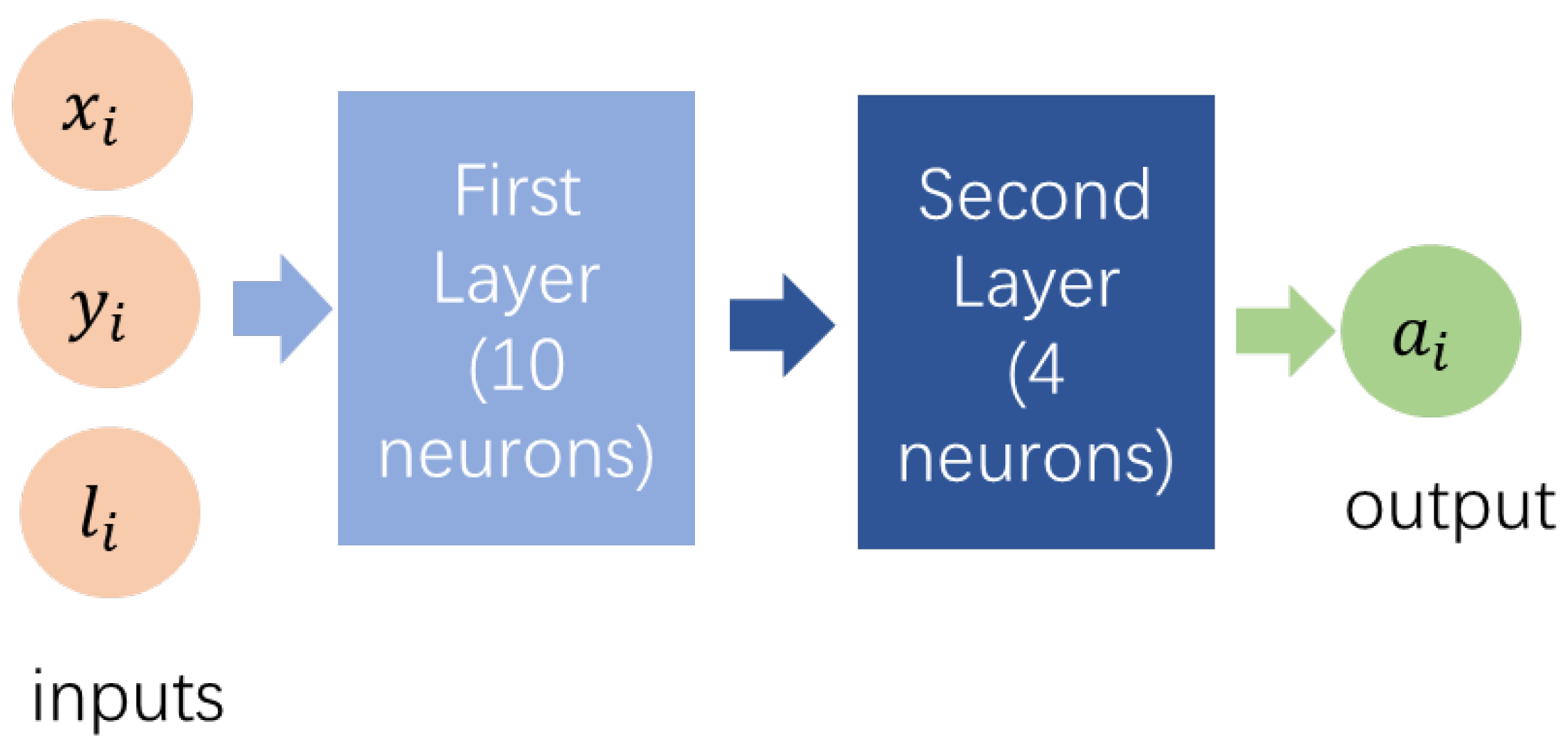
The memory stores the current observation, action, reward, and the next observation $\left(s_i^t,a_i^t,r_i^t,s_i^{t+1}\right)$. In the step, evaluation network and target network are built as shown in Figure 2. The inputs are the robot’s position and the length of the path. The output is the action with the max Q value. The first layer has 10 neurons, and the second layer has 4 neurons. The ReLU activation functions are used in these two layers. In the learning process, the values of the target network and the evaluation network are obtained. The role of the evaluation network is to estimate the maximum Q-value of an action in the target network. The target Q-value is used to train the evaluation network, and this target Q-value is determined by the maximum Q-value from the target network. In addition, samples are prioritized based on the absolute difference between the target network value and the evaluation network value; a larger absolute difference signifies greater potential for improvement in prediction accuracy, making the sample a higher priority for learning. After the training is completed, the absolute difference value will be updated to the memory. The e-greedy value is gradually increased in order to reduce the randomness of behavior. The target Q-value used for training the evaluation network is computed as:

$$Y_i=r_i+\gamma max\widehat{Q}(s_{i+1},a;{\theta }_i^{-})$$

(2)

where $Y_i$ is the target Q-value. $r_i$ is the reward obtained after taking action $a_i$ in state $s_i$. $\gamma =0.9$ is the reward decay factor. ${\theta }_i^{-}$ represents the weights of the target network. To stabilize learning, the target network’s weights ${\theta }_i^{-}$ are periodically updated by copying the weights from the evaluation network $\theta$ after a fixed number of iterations. The number of iterations is defined as 200. This ensures that the target network provides a stable reference for training the evaluation network.

The training data for the DQN will be generated in a simulated environment using Gazebo, as shown in Section 4. The environment consists of a grid map with static obstacles and goal points, where each square represents a navigable space. The data include each robot’s state, defined by its position and path length, the actions taken (move forward, backward; turn left or right), and the corresponding rewards. The reward function assigns a positive value based on the efficiency and safety of the path, penalizes collisions with obstacles, and provides zero rewards for movement in obstacle-free spaces. A prioritized experience replay mechanism stores the robot’s transitions, including the current state, action, reward, and next state, to ensure diverse and informative training samples. The training dataset comprises up to 2000 experiences, sampled in batches of 32 for network updates.

As the number of robots increases, the computation time for task allocation decisions grows, and the complexity of handling path overlaps and collision avoidance becomes more challenging. To address these issues, the system adopts a strategy of map segmentation and robot grouping, distributing the task load across smaller, independent regions to reduce interaction conflicts. Specifically, the global map is divided into multiple sub-maps, each representing a distinct working area. Robots are assigned to specific sub-maps, ensuring that multiple robots do not operate in the same region, thus avoiding path overlaps. Additionally, robots are grouped based on their number, location, and current task states, with each group working exclusively within its designated sub-map. Task allocation within these groups is dynamically managed using the proposed DRL method. This strategy ensures that the number of robots within each sub-map remains manageable, minimizing path overlap issues and reducing the complexity of collision avoidance. Furthermore, the DRL algorithm optimizes task allocation within the segmented sub-maps by leveraging a reward function to prioritize shortest and safest paths. This partitioned management approach significantly improves task execution efficiency while maintaining a high navigation success rate and real-time responsiveness.

3. ROS-Based Fleet Management System Using Reinforcement Learning Algorithm

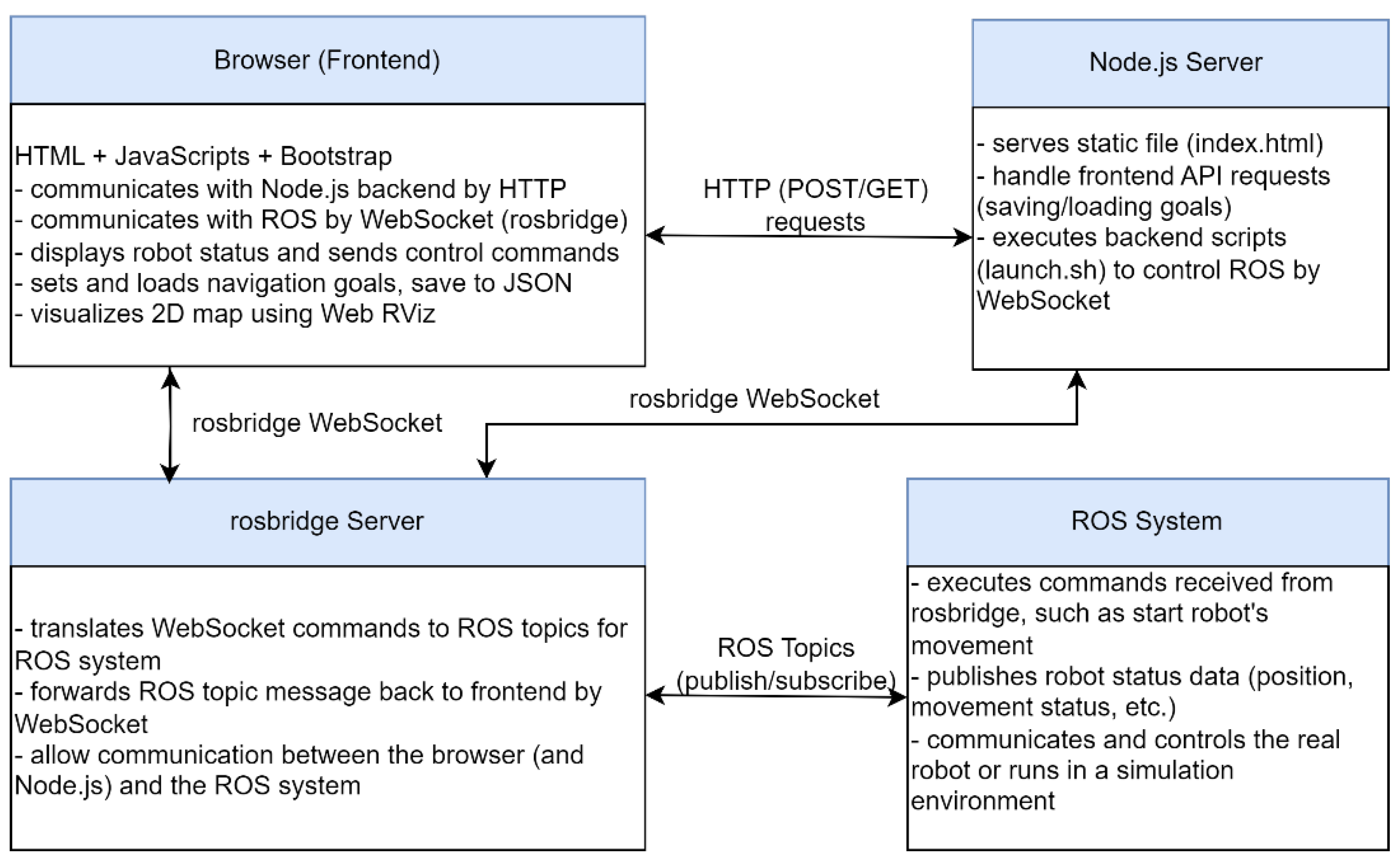
As shown in Figure 3, the system architecture for the multi-robot fleet management system consists of several interconnected layers that work together to efficiently manage and control a fleet of robots. The browser (frontend) serves as the user-facing interface of the FMS, designed with HTML, JavaScript, and Bootstrap-5.3.3 for a responsive and interactive experience. It communicates with the Node.js server via HTTP to handle API requests for saving and loading navigation goals in JSON format and uses WebSocket to interact directly with the ROS system through the rosbridge server for real-time commands and data exchange. Key functionalities include real-time monitoring of robot statuses—such as positions, movement states, and task progress—as well as visualization of a dynamic 2D map using Web RViz, which displays robot locations, paths, and obstacles. Additionally, the interface allows users to set and adjust navigation goals, save them as reusable JSON files, and send control commands to the robots for task execution. This browser interface ensures intuitive and efficient user interaction, enabling real-time task monitoring and management in dynamic multi-robot environments. The Node.js Server serves as the middleware between the frontend and the ROS system. It serves static files, including the index.html, which is the main entry point for the browser interface. The server handles frontend API requests, such as saving and loading navigation goals, ensuring smooth interaction between the user interface and backend data. Additionally, it executes backend scripts like launch.sh to control ROS through WebSocket, managing robot tasks, and initiating specific ROS nodes for robot control and communication. This layer facilitates data exchange and ensures the system’s seamless operation, enabling real-time robot control and task management. The rosbridge server acts as a communication bridge between the browser (frontend) and the ROS system, enabling seamless interaction between non-ROS and ROS components. It translates WebSocket commands received from the browser or Node.js server into ROS topics that the ROS system can process, facilitating real-time control and communication. Additionally, it forwards ROS topic messages, such as robot status updates or navigation progress, back to the frontend via WebSocket for visualization and monitoring. This server plays a crucial role in ensuring smooth and bidirectional communication, allowing the browser and Node.js server to interact effectively with the ROS ecosystem. The ROS System serves as the core operational layer of the fleet management system (FMS), handling direct control and execution of robot tasks. It executes commands received from the rosbridge server, such as initiating robot movements or assigning navigation goals. Additionally, it publishes robot status data, including real-time information on position, movement state, and task progress, which is then relayed to the frontend for monitoring. The ROS system can communicate with and control physical robots or operate in a simulation environment, ensuring seamless transitions between development, testing, and deployment. This layer integrates sensors and actuators to provide real-time feedback and ensure reliable task execution in dynamic environments. These four layers allow the fleet management system to remotely control and monitor a group of robots, providing a comprehensive interface for users to interact with the robots, set goals, and view their operational status.

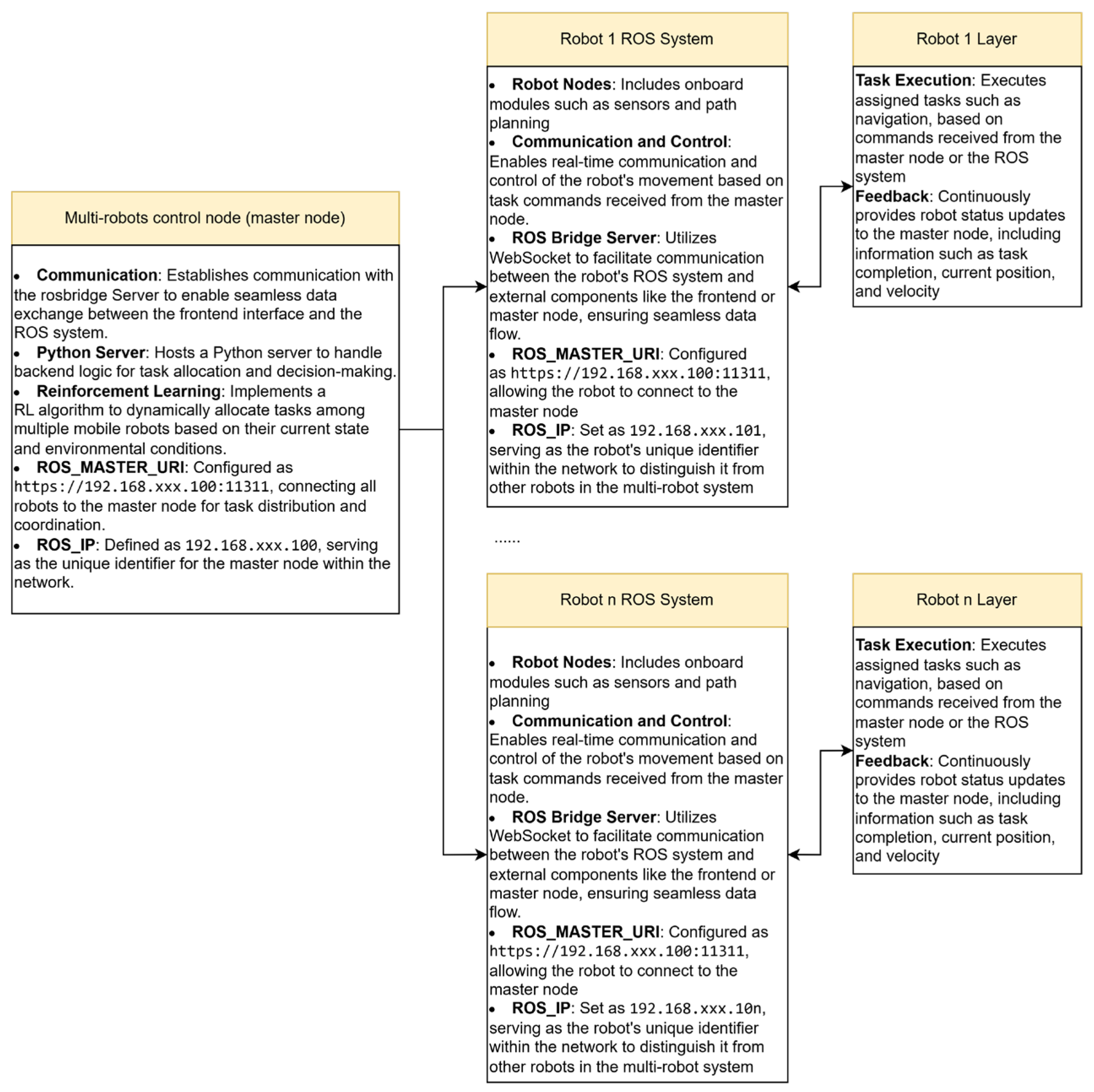
Figure 4 represents a ROS multi-robot control system with DRL algorithm in multiple robot fleet management system. The system consists of a master control node and several slaver robot systems, each with its own ROS system and task execution layer. The master node interacts with a rosbridge server to exchange commands and data between the robots and the central system. In the frontend browser layer of Figure 3, JavaScript code is designed to send a JSON object containing goals to a Python server running at specified URL. It uses the fetch API to make a POST request, handling the server’s response and possible errors. Therefore, in the master node, a Python server is designed to handle an incoming POST request containing JSON data. It saves the received JSON data to a file and logs the data for debugging purposes. This setup provides a robust and dynamic data communication system, even in poor communication environments. In the master node, the DRL algorithm is responsible for task allocation among the robots based on factors like efficiency and safety, ensuring optimal task execution across the fleet, as discussion in Section 2. The DRL algorithm operates as a central decision-making module, receiving each robot’s sensor data and states published through ROS topics. The prioritized experience replay mechanism is implemented to manage historical data to select optimal path. The ROS_MASTER_ URI is the URI that connects all robots to the ROS master. The ROS_IP address of the master node is the same as the ROS_MASTER_URI. For each robot ROS system, the robot nodes include sensor nodes and path tracking nodes, responsible for gathering environmental data. ROS bridge server enables communication with the master node and send the robot’s status to frontend layer in Figure 3. The ROS_MASTER_URI is set the same as the ROS_MASTER_URI in master node, in order to connect to the master node. The ROS_IP address is set as an individual robot’s network IP, allowing it to be uniquely identified within the network. Each robot layer represents the actual task execution and feedback mechanism. The robot completes the assigned task and sends feedback to the master node on its status and task completion.

In the proposed fleet management system, the browser-based user interface leverages WebSocket for real-time monitoring and task assignment. While this design ensures seamless operation under stable network conditions, challenges may arise in environments with unreliable connectivity or limited browser performance. Therefore, a Python Flask server is introduced into the system architecture. The Flask server handles task saving and loading via RESTful APIs, ensuring task data is securely stored and retrievable under various conditions.

4. Results

The training data for the deep Q-network (DQN) was generated in a simulated environment using Gazebo. Depending on the proposed DRL algorithm, three robots plan the safe and shortest paths from their start points to the same goal point individually. As shown in Figure 5, the entire environment is laid out in a grid. Each cell of the grid represents a 1 m × 1 m space that the robot can navigate. The black squares on the grid represent obstacles. The purple square is the goal point for all the robots. The red square, blue square, and gray square are the start points for Robot 1, Robot 2, and Robot 3, separately. Based on the proposed DRL algorithm in Section 2, each robot is trained to optimize its shortest and safest path from its start point to the purple goal point. For the DQN network, each robot’s states and the length of the path are inputs. The max Q-value of one action is output. There are four actions for the robot: move forward, move backward, turn left, and turn right. In the RL algorithm, the learning rate is set as 0.01, which means the robot makes moderate adjustments to the weights with each learning step. If the value is too high, the training might overshoot optimal solutions, and if too low, it might take too long to converge. The reward decay is chosen as 0.9, which means the robot values future rewards slightly less than immediate rewards but still considers long-term benefits. Epsilon is set to 0.9. The target network is replaced with the updated Q-network after every 200 iterations, preventing rapid changes in the network and improving training stability. This approach helps reduce oscillations and divergency during learning. The robot will store up to 2000 experiences. The robot randomly samples 32 experiences from the memory buffer. If the robot collides with the obstacle, the robot is punished −1, and the done value is True. If the robot is the obstacle-free space, 0 is assigned, and the done value is False. If the robot reaches the goal point, the reward value $r_i$ is calculated as (1), and the done value is True. Finally, the red dashed path indicates the shortest and safest path of Robot 1. It moves 10 squares. The blue path represents the shortest and safest path of Robot 2. It moves 8 squares. The gray dashed path shows the shortest and safest path for Robot 3. The robot will move 10 squares. As shown in Figure 5, three robots independently plan paths to the same goal point, navigating through an environment with static obstacles. The selected path is determined based on two primary evaluation factors. The first one is path length. The total distance from the robot’s starting position to the goal point is calculated in terms of grid squares. The shortest path is prioritized to minimize travel time and energy consumption. The second one is path safety. The algorithm evaluates the safety of the path by considering obstacle proximity. Robots that avoid obstacles are assigned higher safety scores. Paths leading to collisions are penalized with negative rewards. Robot 2 was selected for the task as its path covered only 8 squares, the shortest among all robots, and avoided close proximity to obstacles.

As shown in Figure 6, Robot 1’s cost starts at approximately 500, reflecting inefficient decision-making at the beginning of training. Within the first 100 steps, the cost decreases rapidly, demonstrating quick learning as the robot adjusts its actions based on received rewards. By around 500 steps, the cost stabilizes at a consistently low level, indicating that Robot 1 has achieved near-optimal decision-making. Small spikes after stabilization suggest occasional exploration of new actions or adjustments to unfamiliar scenarios. This pattern highlights the robot’s learning progression and convergence toward an effective policy.

Figure 7 represents Robot 2’s cost curve. At the start of the training, Robot 2 has a cost near 60, indicating significant inefficiency or errors in its early decision-making. During the first 1000 training steps, the cost drops steeply, demonstrating that Robot 2 is rapidly improving its performance. Between 1000 and 3000 steps, Robot 2 is still exploring different actions. After 3000 training steps, the cost stabilizes, with values generally hovering around zero. However, compared to Robot 1’s cost curve, there are more frequent and larger fluctuations in Robot 2’s performance even after stabilization. The graph extends to over 4000 training steps, showing that Robot 2 continues to learn over a longer period compared to Robot 1.

Figure 8 shows Robot 3’s cost curve. Robot 3 starts with a high cost, peaking close to 175. Within the first 5000 training steps, the cost drops dramatically. This steep decline indicates that Robot 3 quickly learns to improve its decision-making process and reduces inefficiencies. From around 5000 to 10,000 steps, there are some minor fluctuations, but overall, the cost remains very low, indicating that Robot 3 is consistently making good decisions and performing efficiently. Beyond 10,000 training steps, the cost is almost negligible, approaching zero and remaining flat. This suggests that Robot 3 has effectively converged on an optimal policy and is no longer making significant mistakes.

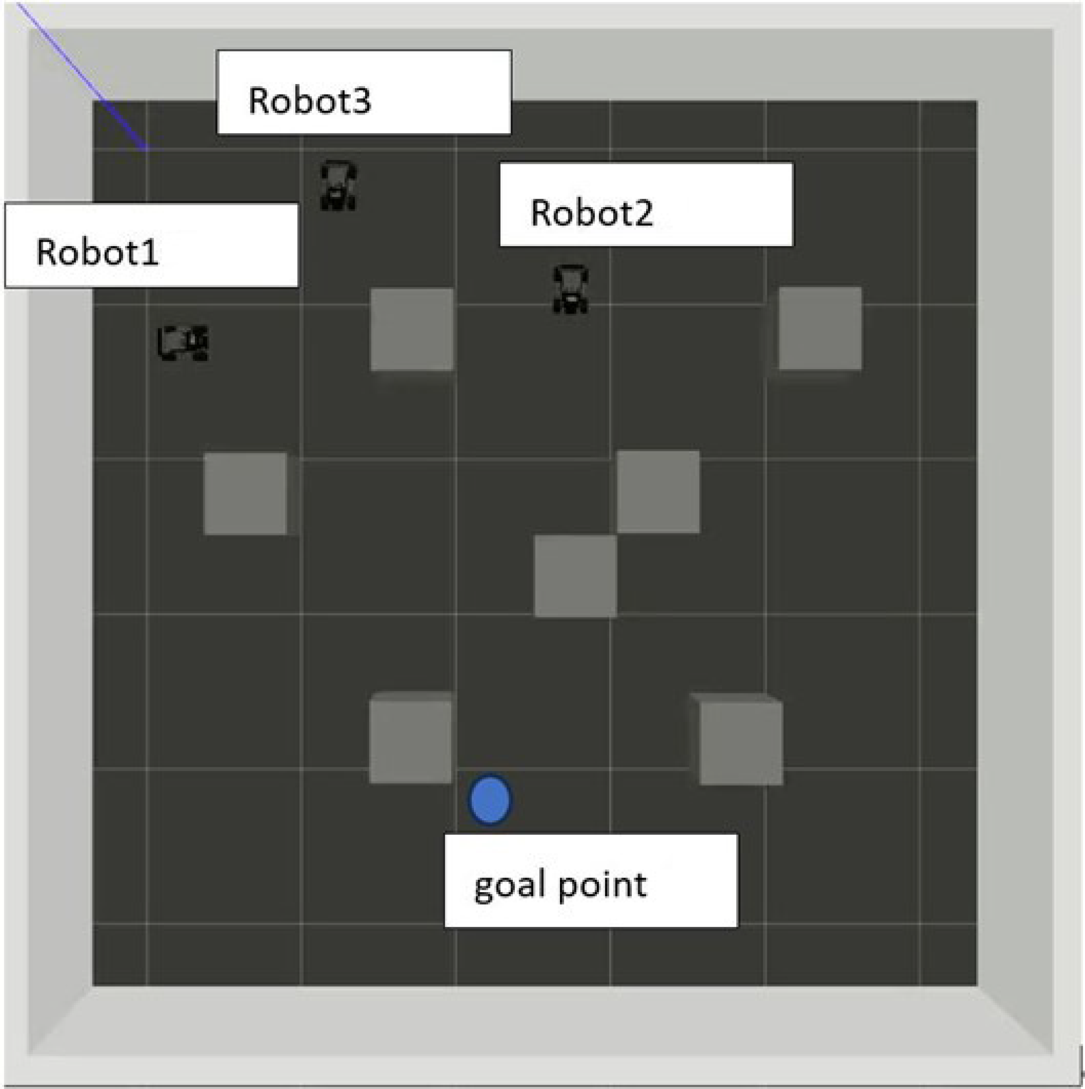
Since the result from Gazebo simulator provides valuable references for practical applications, the proposed algorithms are tested using Gazebo simulator. As shown in Figure 9, three robots are located at their initial position. The blue point is defined as the goal point. The gray boxes are static obstacles. The size of each cell is 2 × 2 m. The robots are equipped with LiDAR sensors. Based on the proposed DQN RL algorithm, Robot 2 has the shortest and safest path to the goal point, so it will finish the mission of moving to the goal point.

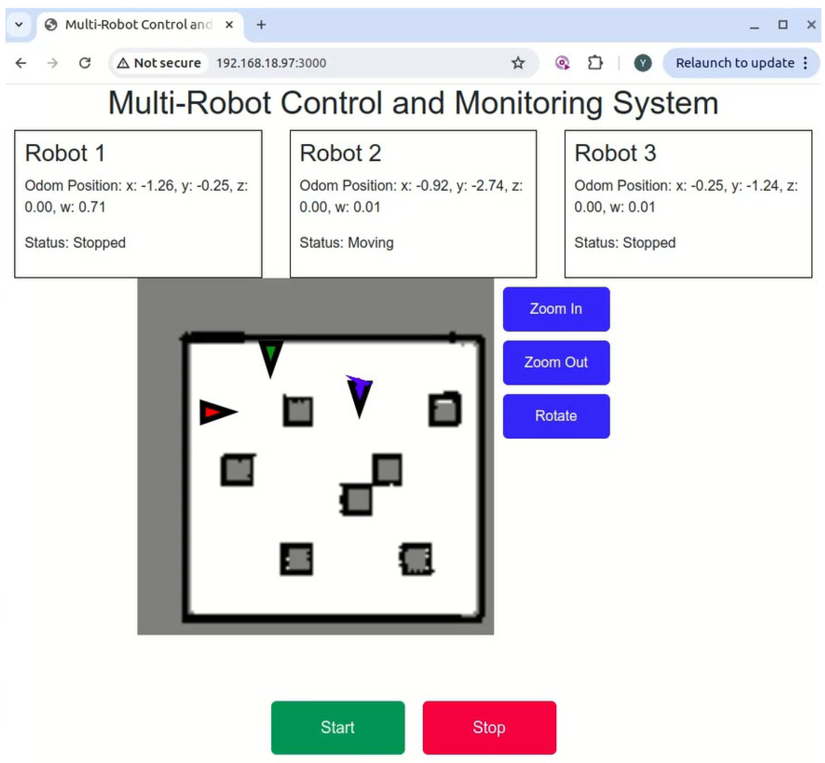
The FMS is designed to control robots and monitor the states of the robots. The Web-based interface is shown in Figure 10. x, y, z, w display the robot’s position and direction. These are provided by the /odom topic. The robot has two motion statuses: stopped and moving. This shows which robot does the mission. Based on the LiDAR data (subscribing/scan topic), the map is built using gmapping algorithm. The system subscribes the/map topic; a 2D map is shown. On the map, the red marker, blue marker, and green marker represent Robot 1, Robot 2, and Robot 3, respectively. If the robot moves, the path will show in the 2D map. The start and stop buttons control start or stop assigning mission to the robot.

The simulation video was uploaded in: https://www.dropbox.com/scl/fi/d7xl8j6i39d2ka1e9eieu/FMS_RL.webm?rlkey=n25b7gt2f0apmpk58l4pyopjw&st=pltxyw7a&dl=0 (accessed on 19 November 2024). The left side is the web-based interface of the FMS system. The right side is the Gazebo simulator environment. The FMS can real-time monitor robots’ status and remotely control robots. In the web-based interface, it shows three robots’ poses. Based on the DRL, after comparing three robots’ shortest and safest paths, Robot 2 should finish the mission of moving to the goal point. Therefore, Robot 2’s motion status is moving, and the others are stopped. For Robot 2, which is marked in blue, the path was drawn in blue line. As shown in Figure 11, at t = 0 s, three robots are at their starting positions, with no path or movement detected. At t = 60 s, Robot 2 avoids the first obstacle and moves towards the goal. At t = 90 s, Robot 2’s path appears optimized to avoid obstacles while heading toward the goal. The robot demonstrates steady movement, adhering to the learned optimal path. At t = 120 s, the robot should avoid two connected obstacles. At t = 150 s, the robot is nearing the goal point, with most of the obstacles successfully navigated. The movement trajectory is streamlined, indicating effective learning from prior steps. At t = 235 s, the robot reaches the goal point successfully. The learning process ensures the robot navigates safely and efficiently, avoiding all obstacles along the way.

Before the robots begin their movements, the system utilizes the DRL algorithm to compute optimal paths for all robots, ensuring the shortest and safest trajectories are identified. In 100 test cases, the average computation time for this initial path planning step was approximately 60 s, as it involves evaluating multiple potential paths for all robots in a static environment. While this initialization step ensures optimal task allocation, the real-time performance of the system remains unaffected, with subsequent dynamic task allocation decisions being completed in an average of 10 ms, demonstrating the system’s capability to handle dynamic and complex multi-robot environments efficiently.

5. Conclusions

This paper introduces a novel multi-robot fleet management system integrating DRL algorithm to address critical challenges in task allocation and path planning in dynamic and complex environments. The primary contribution lies in the deployment of a DQN-based algorithm to enable robots to autonomously learn and adapt their navigation and task strategies, ensuring efficiency and safety in path selection. By integrating a four-layer architecture combining a browser interface, backend processing, and ROS-based control, the system ensures monitoring, communication, and efficient robot coordination. Simulation results highlight the system’s ability to dynamically select one robot to execute a task by comparing path lengths, ensuring both safety and efficiency. The cost curves for individual robots indicate rapid learning, efficient convergence, and effective task policies. The proposed system provides significant advancement in multi-robot coordination and fleet management.