Optimal Fractional-Order Controller for Fast Torque Response of an Asynchronous Motor

Abstract

As high-performance drives, asynchronous motor (AM) drives find extensive use in electric cars, elevators, and machine tools. For these applications, AM drives with direct torque control (DTC) are typically chosen over AM drives with field-oriented control because of their simplicity and quick torque control. Direct torque control of AM drives is frequently achieved using proportional–integral–derivative (PID) controllers. With variable set points and AM parameter ambiguity, these controllers perform poorly. New controllers called fractional-order controllers (FOCs) offer notable improvements over traditional PID controllers due to their enhanced flexibility, robustness, and fine control. In order to provide fast torque performance, this research suggests an AM drive that is regulated by direct torque control theory; nevertheless, the inverter control is optimized for fast response. On the other hand, by employing an optimized fractional-order PI (FOPI) controller, the AM drive speed response is enhanced. The particle swarm optimization (PSO) algorithm is used to optimize the FOPI’s parameters. The MATLAB/Simulink platform was used to model every part of the AM drive with the optimized control system. Three distinct controllers—optimized FOPI, standard PI, and optimized PI—were used to compare the performances of the introduced drive. According to the simulation results, the optimum response in terms of torque and speed was offered by the optimized FOPI controller. The average improvement in the settling time is about 84.4%, and that in the steady-state error is almost killed for all disturbances using the proposed optimized FOPI controller. Furthermore, under parameter uncertainties, the AM’s performance using the suggested optimized FOPI was examined. The outcomes of the simulation demonstrated how resilient the optimized FOPI controller was to changes in the parameters.

1. Introduction

High-performance AM drives have recently found widespread use in contemporary industrial applications, including machine tools, electric cars, elevators, and mine winders. Fast transient response, a broad speed control range, and speed and accuracy are typically needed from high-performance drives [1]. By enhancing the torque responsiveness of the drive, these high-performance AM drive requirements can be satisfied. Two well-known methods—field orientation and DTC—can be used to manage an AM’s dynamic torque [2]. Nonetheless, DTC has numerous benefits over field orientation, including ease of use, high precision, and quick torque response. Furthermore, the DTC process is thought to be resilient to uncertainties in AM parameters [3].

Hysteresis controllers have been used to perform traditional DTC, resulting in a wide range of inverter switching frequencies. This problem complicates the drive inverter’s filter design and raises harmonics [4]. To mitigate the issues provided by hysteresis controllers in conventional DTC, constantly sampled DTC has been suggested. Constant frequency DTC has been the subject of extensive research proposals [5,6,7]. However, only a small number of research studies have taken into account the torque response in DTC [8,9].

The performance of the torque of the AM drives that use DTC has recently been the focus of numerous methodologies and advancements that have been suggested in the literature. Feedback linearization was used to introduce sliding-mode control for DTC-controlled AM drives [10]. DTC-controlled AM drives have adopted the model predictive control (MPC) principles [11,12]. Using a predetermined cost function, MPC determines the optimal inverter state to accomplish the control objectives. The technique has the benefits of great efficiency and low torque and flux ripples. Nevertheless, it has less parameter uncertainty, is complicated, and necessitates several computations. A novel predictive direct torque control method using an optimum modulation technique has been presented in Ref. [13]. Despite having a straightforward concept, the approach has mostly been applied to permanent magnet synchronous motors. In [14], torque ripples, switching loss, tracking speed, and control algorithm complexity parameter variation are critically analyzed. The high-frequency ripples and the comparatively limited range of reference tracking of motor speed are two of the classic controllers’ drawbacks. A predictive controller [12] has been proposed for AMs to address the above-described problems. In order to simplify the controller, a cascaded free control structure is introduced in [15]. For AM drives that use DTC, neural networks and fuzzy approaches have been applied [16,17,18]. An experimental prototype for a twice-supplied AM that is regulated by DTC and optimized by ant colony optimization has been suggested in Ref. [19]. However, the system was complicated and needed to adhere to grid connection system requirements. An optimized fuzzy PID controller, using ant colony optimization, has been adapted for AM drive in [20]. An ideal fuzzy controller for DTC-controlled AM drives has been introduced and designed in reference [21]. Despite its simplicity, the controller produced a lot of noise and had significant torque ripples. To enhance drive performance, Ref. [22] suggested an SVM–DTC method that makes use of a super-twisting sliding mode controller. One technique for controlling the speed in IMs, such as in [23], is adaptive fuzzy sliding mode control. A speed controller for IM utilizing the brain emotional learning intelligent controller (BELBIC) has been developed in [24].

Traditional controllers find it difficult to maintain stability in nonlinear systems because of their variable response under various conditions. This is addressed by fractional-order controllers (FOCs), which give more tuning parameters (fractional orders), increasing flexibility and resilience to nonlinearities such as friction and saturation. Performance in intricate systems, such as power electronics, is improved by this seamless transition between linear and nonlinear systems [25]. Discretization, optimization, and mathematical modeling are all part of designing FOCs for digital implementation. Extending conventional PID regulators to fractional-order PID (FOPID) regulators, in which the integral and derivative parts are both non-integers, is a popular strategy. Optimization-based strategies, frequency response, and improved Ziegler–Nichols policies are examples of tuning procedures. In order to enable real-time implementation for digital control, numerical techniques such as Grünwald–Letnikov and Oustaloup’s approximation are used to estimate fractional derivatives and integrals [26].

Numerous complex systems and drives have used FOCs [27,28,29,30,31]. Actually, the use of FOPID controllers in motor drive control offers notable improvements over traditional PID controllers due to their enhanced flexibility and robustness. Unlike integer-order PID controllers, FOPID controllers allow for fractional differentiation and integration orders, which provides finer control in adjusting the dynamics of the motor system. This adaptability allows FOPID controllers to address system complexities more effectively, handling disturbances and parameter variations with higher precision [27]. Actually, FOPID controllers are preferred over other advanced PID variants (such as sigmoid PID controllers, neuroendocrine PID controllers, piecewise affine PID controllers, PIDA controllers, and many more) due to the merits presented in

Table 1. Summary of the advantages of the FOPID controllers over other advanced PID variants.

Issue	FOPID	PID Variants (Like Sigmoid PID, Neuroendocrine PID, …)	Comments
Flexibility	High	Low	FOPID has two additional parameters (λ and μ) for fractional integration and differentiation, allowing precise control tuning for complex systems.
Robustness	Better	may struggle with large deviations or uncertainties in system dynamics.	Non-integer derivative and integrative components help maintain stability over a broader range.
Frequency Domain	Wide	Narrow
Noise Rejection	Better	Less effective	Due to its fractional-order nature.
Adaptability	Better	Less effective	FOPID’s additional parameters make it more adaptable to diverse application demands compared to fixed-structure controllers like Sigmoid or Neuroendocrine PID [36].
Simplicity	Simple	Moderate	Unlike Neuroendocrine or Sigmoid PID, FOPID avoids computational delays and complexity while retaining performance advantages.

[25,28]. These features fit well with the AM drive system as it is highly nonlinear and includes parameter variations. Also, AM drive systems are usually controlled using variable frequency inverters to achieve wide-speed operation. Hence, the broad frequency domain of the FOPID controllers supports the wide-speed operation of the AM drives. Ref. [29] demonstrated that a FOPID controller enhanced induction motor performance by optimizing time response, proving robust against load changes when tested in a hardware-in-the-loop simulation. Furthermore, FOPID controllers often employ optimization algorithms, such as particle swarm or genetic algorithms, for precise tuning, which is essential for maintaining control accuracy and minimizing error under variable conditions [30]. Ref. [31] provides reliable fractional-order speed controllers for induction motors in low-speed operating zones and with changing parameters. The research is also supported by a hardware-in-loop (HIL) implementation. A novel complex FOC for the speed of an induction motor drive underneath variable working situations with improved robustness has been proposed by [32]. In the speed regulation of sensorless brushless direct current motors, FOPID controllers have been shown to outperform traditional integer-order controllers, particularly in achieving smoother transient responses and better disturbance rejection [33]. Also, FOPID controllers have been applied to nonlinear temperature control systems, delivering improved robustness, stability, faster response times, and greater flexibility when compared to conventional PID controllers [34]. Similarly, the practical implementation and broader applications of fractional-order systems have been explored in recent work [35].

Optimization techniques can be used to tune the suggested FOPI controller parameters [37,38,39,40]. Compared to traditional tuning approaches, these processes resulted in improved system responsiveness and results. However, different algorithms have variable rates of convergence and objective function complexity. Many optimization issues are currently solved using PSO, a metaheuristic optimization method [41]. The PSO algorithm has numerous machine drive applications because of its ease of use and adaptability in implementation [42]. Two cascaded improvements are used to increase the torque and speed performances of the proposed AM drive in contrast to previous attempts. Using a FOPI regulator that has been tuned using the PSO approach, the speed response optimization is the initial step in optimizing the performance. Optimizing the inverter’s functioning to provide a quick torque response is the second optimization step. Additionally, the reactions of three distinct controllers—conventional PI, improved FOPI, and the recently invented AM drive—have been contrasted. Step and ramp speed disturbances have been used to test the introduced drive. Variations in the AM parameters and the reaction of the AM drive to model parameter errors have also been examined. The following were the primary contributions of this study:

• An optimized FOPI regulator has been designed to improve the performance of the proposed AM. It may be regarded as the external optimization process.
• The PSO, a simple metaheuristic optimization technique, has been applied to tune the proposed FOPI controller’s settings to achieve the ideal performance of the AM speed.
• Another optimization process has been implemented for the selection of the inverter’s switching states, to achieve a fast torque response. That optimization process may be considered internal optimization.
• The performance of the suggested drive with the FOPI controller, optimized PI, and the traditional PI were contrasted. A variety of load torque and set speed disturbances was used to evaluate the controller’s performance.
• The AM’s performance using the suggested optimized FOPI was examined under parameter uncertainties.

An AM drive that applies the concepts of DTC is proposed in this manuscript. High torque performance has been achieved by optimizing the power converter’s operation. Conversely, an optimized FOPI is used to optimize the AM drive speed response. The PSO algorithm is used to do the FOPI optimization. There is now a continuous sample of the suggested drive. The MATLAB R2023b (23.2)/Simulink platform has been used to model every part of the AM drive with the optimized FOPI controller. The impacts of the AM parameter uncertainties on the optimization procedures and drive response have been examined, along with comparisons of the responses of the introduced drive utilizing the standard PI and the optimized FOPI controllers.

The following is how the manuscript is prepared. The suggested DTC and the AM’s ideal torque response are described in Section 2. In Section 3, the fractional calculus is revisited. The drive controller’s design and PSO are illustrated in Section 4. Then, Section 5 describes the simulation findings and commentary. Lastly, Section 6 presents the research findings.

2. Direct Torque Control of the Asynchronous Motor

The stator reference frame is an appropriate reference frame for the AM’s DTC. A dynamic model of the AM in the stator reference frame is provided by [43] by assuming infinite permeability of the iron sections and ignoring air gap nonlinearities, iron losses, and slotting effects:

$$\left[\begin{array}{c}\begin{array}{c}{\overline{\mathit{v}}}_s\\ {\overline{\mathit{v}}}_r\end{array}\\ {\overline{\mathit{\lambda }}}_s\\ {\overline{\mathit{\lambda }}}_r\end{array}\right]=\left[\begin{array}{c}\begin{array}{cc}{r}_s+p{L}_s& p{L}_m\\ (p{-j\omega )L}_m& r_r+(p{-j\omega )L}_r\end{array}\\ \begin{array}{cc}{L}_s& L_m\\ L_m& L_r\end{array}\end{array}\right]\left[\begin{array}{c}{\overline{\mathit{i}}}_s\\ {\overline{\mathit{i}}}_r\end{array}\right]$$

(1)

$$M={\displaystyle \frac{P}{3L_m}}·Imj\left\{{\overline{\mathit{\lambda }}}_s{\overline{\mathit{\lambda }}}_r^{*}\right\}$$

(2)

$$J\dot{\omega }=M-\beta \omega -M_l$$

(3)

Commonly, the rotor windings are shorted in cage AMs. Therefore, (${\overline{\mathit{v}}}_r$) will be zero in Equation (1).

The advantages of DTC-controlled AM drives include superior dynamic performance and ease of implementation. They are appealing for high-performance applications that require precise torque control because of these advantages. Hysteresis controllers are typically used in conjunction with traditional DTC. Regretfully, hysteresis controllers choose the voltage vectors without taking the AM’s ideal torque response into account [43]. The inverter operation can be optimized to achieve optimal torque or fast torque response. Therefore, in order to obtain a fast torque response, optimization will be modified for the standard DTC. The torque performance is optimized, and the traditional DTC is evaluated in the paragraphs that follow.

Table 2. The principles of DTC that are utilized in choosing switching states.

Δλ	ΔM	N
		N = 1	N = 2	N = 3	N = 4	N = 5	N = 6
Δλ = 1	ΔM = 1	S2	S3	S4	S5	S6	S1
	ΔM = 0	S7	S0	S7	S0	S7	S0
Δλ = 0	ΔM = 1	S3	S4	S5	S6	S1	S2
	ΔM = 0	S0	S7	S0	S7	S0	S7

presents the DTC principles utilized in choosing the switching states of the inverter.

2.1. Classical DTC Principles of AM

The literature has extensively described the three AM principles of traditional DTC [4]. These indicate that the stator flux and AM torque are independently controlled. By controlling the angle between the stator and rotor flux vectors, torque may be controlled. To track its rated value, the stator flux is typically adjusted. Controlling the stator flux and torque of the IM has been achieved through the regulation of the stator voltage vector selection. As seen in Figure 1, the goal of DTC is to control both the flux and the torque inside a hysteresis window. Thus, the voltage vector selection controls the revolution of the stator flux vector. The following rules are the conventional DTC principles utilized for choosing the inverter switching state [6]:

• The stator flux vector is rotated by active switching states, which causes the torque and flux to change.
• The flux will be stationary, and the torque will be reduced because zero switching states halt the stator flux vector’s motion.
• There are two adjacent active voltage vectors for each zone within the switching states axes shown in Figure 1 that can be utilized to boost torque. But one causes the flux to increase, while the other causes it to decrease. For example, in sector (2), the torque can be increased by choosing either vector S₂ or S₃. Conversely, the stator flow is increased by S₂ and decreased by S₃.

2.2. Optimized Operation of the AM Converter

The optimization technique must concentrate on choosing the switching state that produces the highest torque rate in order to obtain a quick torque response from the IM. The torque rate equation as a function of the stator switching states is created as the initial step in the optimization process. Therefore, it is necessary to determine the relationship between the applied switching state and the AM’s torque rate. When the AM-generated torque (2) is differentiated by time, the following results are obtained [4]:

$$\dot{M}={\displaystyle \frac{P}{3L_m}}·Imj\left\{\dot{{\overline{\mathit{\lambda }}}_s}\overline{{\mathit{\lambda }}_r^{\mathbf{*}}}+{\overline{\mathit{\lambda }}}_s\dot{\overline{{\mathit{\lambda }}_r^{\mathbf{*}}}}\right\}$$

(4)

During the stator voltage vector’s operational period, it is anticipated that the rotor flux vector will rotate with a constant angular speed and amplitude. This assumption stems from the fact that the rotor flux is steady and varies more slowly than the stator flux since the rotor time constant for the standard AM is usually greater than 100 ms [8]. On the other hand, the relationship between the stator voltage vector and the stator flux vector, ignoring the stator resistance, is as derived in [4]. As a result, the rotor and stator flux vectors can be expressed as follows:

$$\left[\begin{array}{c}{\overline{\mathit{\lambda }}}_r\\ {\overline{\mathit{\lambda }}}_s\end{array}\right]=\left[\begin{array}{c}{\lambda }_r\angle -(\omega t+{\theta }_{ro})\\ {\overline{\lambda }}_o+{\overline{\mathit{V}}}_{n}t\end{array}\right]$$

(5)

When we differentiate Equation (5) about time, we obtain the following:

$$\left[\begin{array}{c}\dot{{\overline{\mathit{\lambda }}}_r}\\ \dot{{\overline{\mathit{\lambda }}}_s}\end{array}\right]=\left[\begin{array}{c}-j\omega {\overline{\mathit{\lambda }}}_r\\ {\overline{\mathit{V}}}_n\end{array}\right]$$

(6)

Equations (5) and (6) can be substituted into Equation (4) to produce the following:

$$\dot{M}=P·Imj\left\{{(\mathit{V}}_n-j\omega ({\mathit{V}}_{n}t+{\overline{\mathit{\lambda }}}_o))\overline{{\mathit{\lambda }}_{\mathit{r}}^{\mathit{*}}}\right\}/3L_m$$

(7)

By simplifying Equation (7) and letting t = 0 (the time of applying the next voltage vector):

$$\dot{M}=P{\lambda }_r\left[Vsin({\theta }_n-{\theta }_{ro})-\omega {\lambda }_{o}cos({\theta }_n-{\theta }_{ro})\right]/3L_m$$

(8)

Allow

$$\phi ={tan}^{-1}\left({\displaystyle \frac{\omega {\lambda }_o}{V}}\right)$$

(9)

Therefore, we obtain the following:

$$\dot{M}=C_{1}sin({\theta }_n-{\theta }_{ro}-\phi )$$

(10)

where (C₁) is a constant.

Equation (10) should be adjusted for the available voltage vectors in order to achieve the greatest torque rate or fastest torque response. According to Equation (11), the cost function (ξ) is:

$$\xi =\underset{n}{\max }\left[sin\left({\theta }_n-{\theta }_{ro}-\phi \right)\right]$$

(11)

An observer should be used to determine the motor speed, rotor flux, and stator flux in order to carry out the optimization procedure. Unfortunately, the AM parameters used by the observer are considered unclear. The simulation results section takes into account how the AM parameters’ uncertainty affects the suggested drive performance.

3. Fractional Calculus: An Overview

Fractional calculus represents a branch of mathematical analysis that provides a generalized framework for modeling natural phenomena more accurately, avoiding the limitation of traditional differential calculus, which assumes integer-order derivatives. This approach involves taking the power of differential and integration operators to real numbers, broadening the scope of applications and enabling more precise modeling of complex systems [25]. The generalized differ-integral can be expressed as follows [25]:

$${}_{c}D_t^{a}f\left(t\right)={}_{c}I_t^{-\alpha }f\left(t\right)=D_{t-c}^{\alpha }f\left(t\right)={\displaystyle \frac{d^{\alpha }f\left(t\right)}{{\left[d\right(t-c\left)\right]}^{\alpha }}}=\left\{\begin{array}{c}{\displaystyle \frac{d^{\alpha }f\left(t\right)}{d{t}^{\alpha }}}, \alpha >0\\ 1, \alpha =0\\ {\int }_c^{t}f\left(t\right)d{t}^{-\alpha }, \alpha <0\end{array}\right.$$

(12)

where α ∈ R+ represents the real order of the differ-integral, t is the variable with respect to which the differ-integral is taken, and c is the lower limit, typically c ≥ 0 for causal systems. Several alternative definitions exist for fractional-order integrals and derivatives. The three most widely recognized definitions of fractional derivatives and integrals are the Grünwald–Letnikov (GL), Riemann–Liouville (RL), and Caputo (C) definitions, provided in the time domain as follows:

▪

Grünwald–Letnikov definition:

$${}_c{}^{\mathit{GL}}D_t^{a}f\left(t\right)=\underset{h\to 0}{\lim }{h}^{-\alpha }\sum _{j=0}^{N-1}{\left(-1\right)}^j.\left({\displaystyle \genfrac{}{}{0pt}{}{\alpha }{j}}\right).f(t-j.h)$$

(13)

where $N=\left[{\displaystyle \frac{t-c}{h}}\right]$ considers the maximum boundary of the computational universe, [·] is the integer part, h considers a grid size, and $\left({\displaystyle \genfrac{}{}{0pt}{}{\alpha }{j}}\right)$ is a binomial coefficient.

▪

Riemann–Liouville definition is given by the generalized form:

$${}_c{}^{\mathit{RL}}D_t^{a}f\left(t\right)={\displaystyle \frac{1}{\Gamma (n-\alpha )}}{\left({\displaystyle \frac{d}{dt}}\right)}^n\underset{c}{\overset{t}{\int }}{\displaystyle \frac{f\left(t\right)}{{(t-\tau )}^{1-(n-\alpha )}}}d\tau , \left(n-1\right)<\alpha <n$$

(14)

where (Γ) is the Euler Gamma function.

▪

Caputo’s definition, also known as the smooth fractional derivative, stated

$${}_c{}^{C}D_t^{a}f\left(t\right)={\displaystyle \frac{1}{\Gamma (n-\alpha )}}\underset{c}{\overset{t}{\int }}{\displaystyle \frac{f^n\left(\tau \right)}{{(t-\tau )}^{1-(n-\alpha )}}}d\tau , \left(n-1\right)<\alpha <n$$

(15)

By the definitions of Riemann–Liouville and Grunwald–Letnikov, one sees that derivatives of fractional order are global operators, which preserve the memory of all past events. That is an important property for modeling hereditary and memory effects within a wide class of materials and systems. Concerning the numerical calculation of the fractional-order derivative, the next formula, Equation (12), can be used which is obtained by the GL definition. This methodology relies on the premise that for a broad category of functions, GL (Equation (13)), RL (Equation (14)), and Caputo’s definitions (Equation (15)) exhibit equivalence [44]. Additionally, the fractional-order derivative and integral can be articulated within the context of the transformation domain. It has been demonstrated that the Laplace transform corresponding to a fractional derivative of a function $f\left(t\right)$ is expressed as

$$\mathcal{L}\left\{D_t^{\pm \alpha }f\left(t\right)\right\}=s^{\pm \alpha }.\underset{F\left(s\right)}{\underbrace{\mathcal{L}\left\{f\left(t\right)\right\}}}-\sum _{k=1}^{n-1}{s}^k.\underset{Initial function}{\underbrace{\left({}_0{D}_t^{\pm \alpha -k-1}f\left(t\right){|}_{t=0}\right)}}$$

(16)

Since null initial conditions have been considered for the problem, Equation (16) is simplified into the form:

$$\mathcal{L}\left\{D_t^{\pm \alpha }f\left(t\right)\right\}=s^{\pm \alpha }.F\left(s\right)$$

(17)

Due to the analytical and synthetic simplicity, the Laplace transform has been demonstrated as an indispensable means for the investigation and design of fractional-order control structures [45]. Extensive information about the numerical methods of the simulation and discretization of the fractional-order systems can be found in [46,47].

3.1. The Proposed FOPID Controller Approximation and Discretization of the Fractional Operators: An Overview

The ideal digital fractional-order differentiator-integrator ${}_0{D}_t^{\pm \alpha }$ defines a discrete-time system in which the output $y\left(n\right)$ is a uniform sampling of the ${\alpha }^{th}$ order derivative of f(t). Hence, if α > 0, we have

$$y\left(n\right)={}_0{D}_t^{\pm \alpha }f\left(t\right){|}_{t=nh}$$

(18)

Generally, when a function $f\left(t\right)$ is estimated using a grid function, $f(n.h)$, with h representing the discretization period (the calculation step size or sampling interval), the approximation for its fractional derivative order α can be articulated as [25].

$$y_h\left(nh\right)={\displaystyle \frac{d^{\pm \alpha }f\left(t\right)}{d{t}^{\pm \alpha }}}=\underset{h\to 0}{\lim }{h}^{\mp \alpha }.{\left[∆f\left(t\right)\right]}^{\pm \alpha }=h^{\mp \alpha }.{\left(w\left({\zeta }^{-1}\right)\right)}^{\pm \alpha }.f_h(n.h)$$

(19)

where $∆f\left(n-h\right){|}_{t=n.h}=f\left(n.h\right)-f\left(n.h-h\right)$, ζ⁻¹ is a shift operator and $w\left({\zeta }^{-1}\right)$ is a generating function (GF). This generating function with its expansion defines the structure of the approximation and the coefficients, too [42].

Several different approaches for approximating fractional derivatives and integrals have been developed.

• Methods that rely on calculating analytical expressions for the derivative and integral of a signal—known as temporal analysis—are widely applied in this context. Among these, the GL (Grünwald–Letnikov) and the Adams–Bashforth–Moulton (ABM) algorithms, both derived from Caputo’s definition, are especially popular.
• Methods that approximate a fractional model with a rational continuous-time model that is known as frequency analysis. For this purpose, the Laplace transform is the commonly used approach.

From the signal processing and control viewpoint, the ABM and GL methods provide the most practical and important approaches for discrete-time application. Additionally, in control system design and analysis, the Laplace transform method is commonly employed. Consequently, the synthesis of a fractional-order controller is ideally performed in the frequency domain. For this reason, frequency response data serves as the foundation for the majority of design techniques suggested for FOC.

3.2. The FOPID Controller

The reason for using the digital FOPID controller is that classical (analog) PID controllers are the most common class of industrial controllers, such that continuous efforts are made to enhance their performance and robustness. The classical PID includes a proportional controller (with gain K_P), an integral controller (with gain K_I = K_P.T/Ti), and a derivative controller (with gain K_D = K_P.T_d/T), which are all dependent on the error signal, and it can be presented in continuous form and formulated in discrete time as

$$M_{ref}\left(x{|}_{x=n.T}^{x=t}\right)\left|\begin{array}{c}\stackrel{P-action}{\overbrace{K_p.e\left(t\right)}}+\stackrel{Integral action}{\overbrace{K_I.D_t^{-1}e\left(t\right)}}+\stackrel{Derivative action}{\overbrace{K_D.D_t^{+1}e\left(t\right)}}\\ K_p.e\left(n.T\right)+K_I.T{\sum }_{j=0}^{n}e\left(jT\right)+K_D.(e\left(n.T\right)-e\left(\left(n-1\right).T\right))/T\end{array}\right.$$

(20)

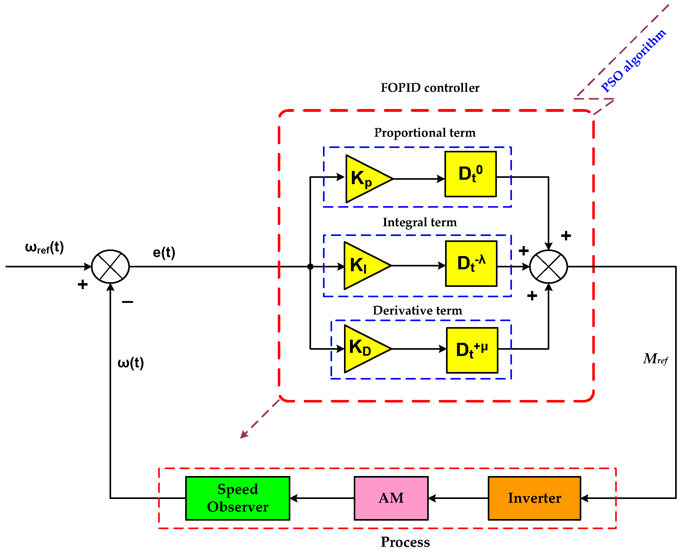
Equation (20) can be extended to a fractional controller that includes an integrator of order λ ∈ R+ and a differentiator of order μ ∈ R+ [45]. Figure 2 shows the schematic diagram of the FOPID control loop.

It can be represented in both continuous and discrete time by the mathematical model of the FOPID controller given by

$$M_{ref}=\left\{\begin{array}{c}{K}_P.e\left(t\right)+K_I.D_t^{-\lambda }e\left(t\right)+K_D.D_t^{\mu }e\left(t\right)\\ K_P.e\left(n.T\right)+K_I{∆}_{n.T}^{-\lambda }e\left(n.T\right)+K_D.{∆}_{n.T}^{\mu }e(n.T)\end{array}\right.$$

(21)

The execution of the control loop involves essentially three steps:

• The first objective is to develop an analysis framework of the controller by using discretization techniques and approximation of fractional-order operators.
• The second objective is to evaluate the developed knowledge base for the identified controller structure by implementing learning and optimization algorithms.
• The final stage for the proposed algorithm is the validation of its coherence through real-time implementation.

Frequency-domain analysis is the most commonly used approach in designing the FOC, where the continuous transfer function of the FOPID controller is derived using the Laplace transform or the discrete z-transfer function.

The Laplace transform of the system’s transfer function, with E(s) as the error signal input and U(s) as the controller’s output, is given by

$$G_c\left(s\right)={\displaystyle \frac{U\left(s\right)}{E\left(s\right)}}=K_P+K_I.s^{-\lambda }+K_D.s^{\mu }, \left\{\lambda ,\mu \right\}>0$$

(22)

Discrete transfer function given by the following expression:

$$G_c\left(z\right)=K_P+K_I.{\left(\psi (z^{-1}\right))}^{-\lambda }+K_D.{\left(\psi (z^{-1}\right))}^{\mu }, \left\{\lambda ,\mu \right\}>0$$

(23)

Here, $s\to \psi \left(z^{-1}\right)$ is the discrete operator, which can be represented as a function of the complex variable z or the shift operator z⁻¹. The discrete-time correspondence of the fractional differentiation-integrator $s^{\pm \alpha }$ should be ${\left(\psi (z^{-1}\right))}^{\pm \alpha }$.

In recent years, FOPID controllers have garnered significant attention from both academic and industrial fields. However, due to the inherent complexity of fractional-order systems, existing control design techniques for these systems often lack direct, systematic approaches that allow for fair comparison with traditional integer-order controllers [48].

Adjusting the FOPID controller involves fine-tuning five key parameters K_P, K_I, K_D, λ, and μ. This expanded parameter set offers enhanced flexibility and precision in control system design. Analytical methods, such as the internal model control approach, extend traditional PID tuning techniques to accommodate the fractional orders in FOPID controllers, deriving parameters that achieve desired closed-loop behavior and robustness [49]. Optimization algorithms, including PSO and genetic algorithms, are employed to fine-tune FOPID parameters, effectively enhancing stability and transient response [50]. Auto-tuning techniques, utilizing relay feedback tests, automatically adjust controller parameters in real-time, simplifying the tuning process and adapting to system changes [26]. Each method offers unique advantages, and the choice depends on specific system requirements and constraints.

To ensure the practical applicability and robustness of the proposed FOPID controller, specific constraints have been introduced to mitigate potential risks, particularly regarding the integral term. These enhancements include the following:

• Anti-Windup Mechanism:
  To address the risk of integral windup, a saturation block has been incorporated into the integral term. This mechanism prevents the accumulation of excessive error, ensuring that the controller maintains stable and effective operation under large disturbances or prolonged error conditions.
• Constraints on Fractional Orders (λ and μ):
  The fractional orders of integration (λ) and differentiation (μ) are constrained within the range [0.1, 1]. This range strikes a balance between flexibility and stability, avoiding impractical configurations that could lead to instability or degraded performance.

In the proposed system, there is no derivative term. However, if it is present, a low-pass filter has to be applied to the derivative term to attenuate high-frequency noise, which is often amplified by fractional-order derivatives. This filtering improves robustness, particularly in noisy environments, and ensures smoother system responses.

The constrained FOPID controller exhibits reduced overshoot, faster settling times, and enhanced robustness under varying operating conditions compared to the unconstrained design.

4. Construction and Optimization of the Drive Controller

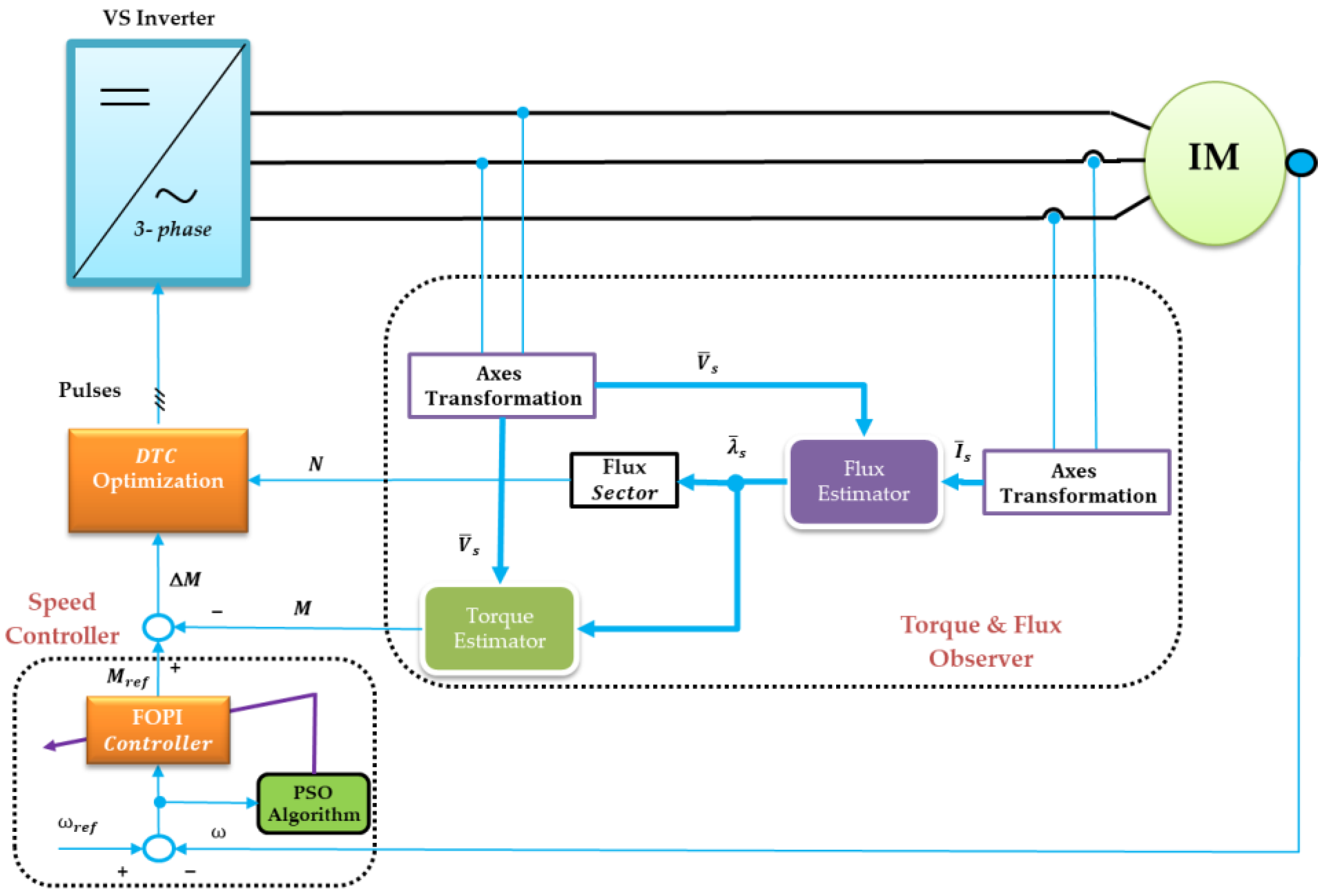
Figure 3 shows a block schematic of the newly developed AM drive with the optimized controller. The suggested system has two optimizations. The speed controller parameter optimization is implemented for the outside loop optimization. It optimizes the speed controller’s performance by applying the PSO algorithm. Nevertheless, according to Equation (11), the next optimization is applied to the interior loop that optimizes the inverter states to attain a rapid torque response. The speed controller, which is the primary controller, creates the outer loop by comparing the commanded and measured speeds, generating the error that is regarded as the regulator’s entered signal. An optimized FOPI regulator is utilized for that job. The PSO algorithm is utilized to optimize the controller. The speed controller’s output serves as the torque loop’s set point and the AM’s reference torque. However, the inner loop is a torque loop that is controlled using optimized DTC. It makes up the inner loop where a different optimization procedure is modified to provide a quick torque response. The AM voltage source inverter’s ideal voltage vector is output by the controller. The following part will describe the control system.

4.1. The A.M. Control Procedure

Digital controllers with constant sampling time are part of the suggested AM control system. The AM model equations, along with the measured currents and speed, are used to develop estimators for the stator flux, AM torque, and rotor flux angle. Figure 3’s optimization process uses the torque error (ΔM) and the calculated parameters using observers as inputs.

The optimization flowchart of the switching states is presented in Figure 4. The speed controller loop is the outer loop. Its FOPI controller is optimized, as will be discussed in the next section.

4.2. Particle Swarm Optimization (PSO) Technique

PSO [51] is a population-based search algorithm where the solutions, called particles, are randomly initialized. Each particle is characterized by a position and a velocity. Particles fly through the search space and their velocities are dynamically adjusted based on past experiences. In PSO, the velocity of each particle determines its flight path in the search space; thus, the method is particularly suited for various optimization problems.

The position of the ith particle in a D-dimensional search space can be represented by a vector $X_i={[x_{i1},x_{i2},\dots ,x_{iD}]}^T$ in the D-dimensional space. The velocity of the above particle can be related to another vector, given by $V_i={[v_{i1},v_{i2},\dots ,v_{iD}]}^T$ in the same D-dimensional space. In addition, the best position encountered so far by particle i can also be mapped to a D-dimensional vector represented as $P_i={[p_{i1},p_{i2},\dots ,p_{iD}]}^T$. The best-performing particle over all of the population is usually referred to as the “global best” and is typically used in guiding the movements of other particles.

Two key equations govern the evolution of the swarm:

$$v_{id}^{h+1}=w_i^{h+1}{v}_{id}^n+a_1{r}_1^h\left(P_{id}^h-x_{id}^h\right)+a_2{r}_2^h(P_{gd}^h-x_{id}^h)$$

(24)

$$x_{id}^{h+1}=x_{id}^h+v_{id}^{h+1}$$

(25)

where $d=\mathrm{1,2},\dots ,D$; $i=\mathrm{1,2},\dots ,Q$, and Q is the size of the swarm (i.e., number of particles in the swarm); $a_1,a_2$: positive values, called acceleration constants; $r_1,r_2$: random numbers uniformly distributed in [0, 1]; $h=\mathrm{1,2},\dots ,H$ determines the iteration number, H is the maximal times of iteration; $y$: is the inertia weight function, denoted as

$$y^h={\displaystyle \frac{0.5h}{1-H}}+{\displaystyle \frac{0.4-0.9H}{1-H}}$$

(26)

“y” varies linearly from 0.9 to 0.4 within the iterations, balancing the global and local search capabilities of the algorithm. A large inertia weight value supports the global search, whereas a small value provides a better local search.

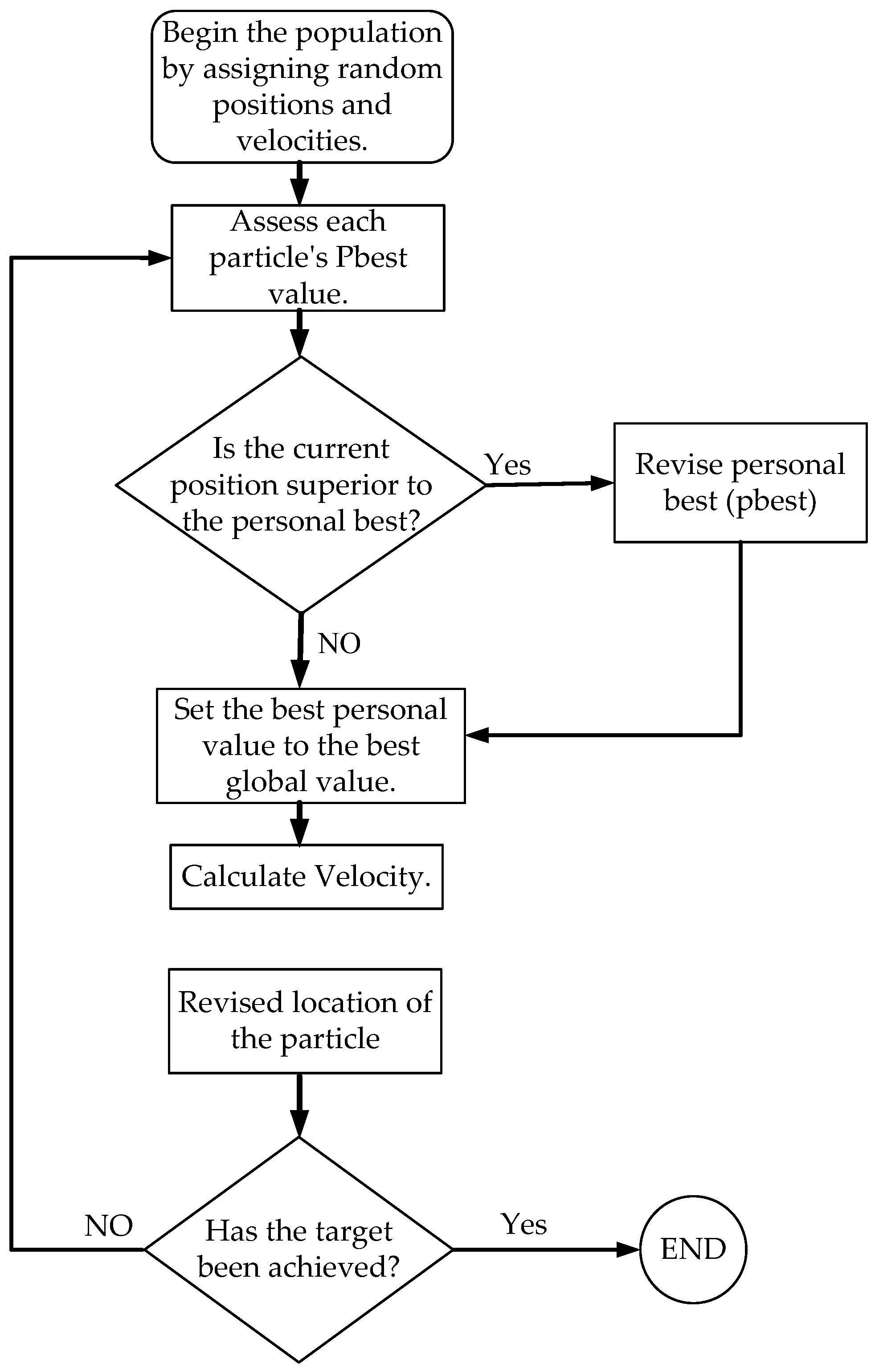
The PSO algorithm proceeds as follows:

• Initialization: A swarm of particles is initialized with random positions and velocities in the D-dimensional problem space, where each particle represents a potential solution. The dimensions correspond to the FOPI controller parameters: K_p: proportional gain.
  • K_I: Integral gain.
  • λ: Order of the integral term.
  • μ: Order of the derivative term.
• Fitness Assessment: The fitness function is defined as the Integral of Time-weighted Absolute Error (ITAE):

  $$ITAE={\int }_0^{T_s}t.\left|e\left(t\right)\right|dt={\int }_0^{T_S}\left|\left(\omega -{\omega }_{ref}\right)\right|·\mathrm{t}dt$$

  (27)

  where e(t) is the error between the reference speed and the actual speed of the motor. Lower fitness values indicate better solutions.
• Personal Best Update: Each particle tracks its best position (personal best, $Pbest$) based on the fitness value. If the current fitness of a particle is better than its personal best, $Pbest$ is updated to the current position.
• The Global Best Update: The best-performing particle across the entire swarm is identified as the global best ($gbest$). The corresponding position in the four-dimensional space $(K_p,K_i,\lambda ,\mu )$ is stored and used to guide the swarm’s movement.
• Velocity and Position Update: The velocity and position of each particle are updated using the formulas Equations (24) and (25).
• Termination: Steps 2–5 are iterated until a termination criterion is met, such as reaching a desired value of fitness threshold (e.g., a sufficiently low ITAE value) or completing a maximum number of iterations.

Figure 5 illustrates a flowchart of how the PSO algorithm works.

The corresponding parameters of the PSO are as follows: the personal best coefficient (C₁) = 1.5, global best position (C₂) = 1.5, Q = 10, the maximum number of iterations = 20, inertia weight (y) = 0.6, and number of particles = 10. In our study, we use the ITAE as the primary optimization criterion, as presented in Equation (27). By prioritizing ITAE, the cost function improves system response by reducing both the size and duration of errors, helping the system stabilize more quickly. The parameters of the PI, the optimal PI, and the optimized FOPI are presented in

Table 3. The controllers’ settings.

Variable	PI	Optimal PI	FOPI
Kp	5.8	10.853	3883.591
KI	1.6	1.9531	120.3078
λ	0	0	0.014168

. The very low objective function estimate can be obtained using the suggested PSO technique. Furthermore, it is noteworthy that the PSO technique can approach the optimal gains in a relatively short length of time, typically within 20 iterations, when taking the objective function (ITAE) into consideration.

$$ITAE={\int }_0^{T_S}\left|\left(\omega -{\omega }_{ref}\right)\right|·\mathrm{t}dt$$

(28)

Table 3 highlights the optimized parameter values for the PI, optimal PI, and FOPI controllers. The PSO algorithm successfully optimized the FOPI parameters, including the fractional orders λ and μ, resulting in improved control performance. These optimized values enable finer control of the system’s dynamics and provide enhanced robustness against parameter variations.

Figure 6 illustrates the convergence behavior of the PSO algorithm used to optimize the FOPI controller. The algorithm achieves rapid convergence within 20 iterations, demonstrating its efficiency in finding optimal parameter values. The steep initial descent in the curve indicates the effective exploration of the solution space, while the subsequent stabilization reflects the fine-tuning of the parameters to minimize the fitness function (ITAE).

4.3. Statistical Analysis of PSO Performance

To validate the consistency and effectiveness of the PSO algorithm in optimizing the FOPI controller parameters, 10 independent trials were conducted under identical conditions. The fitness function ITAE was used to assess the performance of each trial. The best ITAE value obtained across all trials was 4.7081 × 10⁴, reflecting the most optimal result.

The average ITAE across the 10 trials was 4.9904 × 10⁴, with a standard deviation of 2.745 × 10³, indicating minimal variability and high consistency in the optimization process. Additionally, the 95% confidence interval for the ITAE values ranged from 4.5442 × 10⁴ to 5.6009 × 10⁴, further confirming the robustness of the PSO algorithm in producing stable and reliable results despite its inherent stochastic nature.

These statistical results demonstrate that the PSO algorithm consistently produces near-optimal solutions for the FOPI controller parameters, ensuring reliable performance even across multiple trials. The narrow confidence interval further underscores the reliability of the optimization process within the given conditions.

Table 4. The statistical analysis of ITAE values across 10 trials.

Metric	Value
Mean ITAE	4.9904 × 104
Standard deviation	2.745 × 103
Minimum ITAE (Best)	4.7081 × 104
Maximum ITAE	5.6009 × 104
95% Confidence Interval	[4.5442 × 104, 5.6009 × 104]

presents the statistical analysis of ITAE values obtained from 10 independent trials of the PSO-optimized FOPI controller, summarizing key metrics derived from the ITAE evaluations.

Table 5. Comparison of error objective functions for three controllers.

Function	PI	Optimal PI	FOPI
ITAE	92.8552	82.0838	12.0912
IAE	42.2782	32.2508	17.3564
ISE	599.5835	492.6784	427.5514
TAE	126.8486	82.1069	12.1068
SSE	2.924	1.4918	4.0296 × 10−6

provides a detailed comparison of the performance of three controllers PI, optimized PI, and optimized FOPI—using various error objective functions. These objective functions evaluate the accuracy and efficiency of the controllers in minimizing system errors and achieving robust performance.

The results demonstrate the superiority of the FOPI controller across all metrics. The FOPI controller achieves significantly lower ITAE, IAE, and TAE values compared to the PI and optimal PI controllers, indicating enhanced transient and overall performance. Additionally, the FOPI controller exhibits near-zero SSE (4.0296 × 10⁻⁶), underscoring its precision in achieving steady-state accuracy. These findings highlight the advantages of fractional-order control techniques in improving control system performance.

5. Discussion of the Simulation Results

MATLAB/Simulink is used to mimic the suggested AM control system using the optimized FOPI controller, as seen in Figure 3. With the settings listed in

Table 6. The suggested AM drive settings.

Variable	Value
Ls, Lr, Lm	42.4, 41.7, 41 mH
Rr, Rs	156, 294 m Ω
J	0.4 kgm2
λs	454 mWb

, the AM power rating is 10 KW, the number of poles is six, the voltage rating is 220 V, and the frequency is 60 Hz.

The PSO-optimized FOPI controller and the traditional PI controller have been compared. Nonetheless, all the controllers have maintained the same internal optimization loop, which is utilized for the quick torque response. The load torque (M_l) is considered as the system disturbance, while the reference speed (ω_ref.) is the input set point. Figure 7a displays the results obtained under ramp and step changes in the reference speed. Furthermore, as Figure 7b illustrates, there were load torque irregularities. Figure 7c compares the AM speed responses with the two controllers. The best speed response is unquestionably provided by the PSO-optimized FOPI controller. Its steady-state error and settling time are the lowest without overshooting. The conventional PI controller has the worst response. At all disturbances, it exhibits the biggest steady-state inaccuracy, overshoot, and settling time. With the traditional PI and FOPI controllers, the steady-state error value fluctuates with the disturbances but is not constant. Furthermore, it is noted that with the suggested controller, the AM speed is hardly impacted by the sharp increases in the demand torque at the timings (1.5 s, 3 s, 5 s, and 6.5 s). However, with the traditional PI controller, these demand torque variations result in mild transients and marginally increased steady-state errors. Profiles of the % speed errors for both controllers are displayed in Figure 7d. The speed error profile is lowest using the PSO-optimized FOPI regulator. When compared to the traditional PI regulator, it is evident that the new controller—the PSO-optimized FOPI—has better performance. Comparing the proposed controller to the FOPI controller and the traditional PI, the speed errors, such as the IAE, of the AM speed have decreased by roughly 4%.

Figure 8 shows the AM performance characteristics utilizing the PSO-optimized FOPI controller and the traditional PI controllers under the same disturbances as before. Figure 8a–d display the AM currents utilizing the improved FOPI controllers and the conventional PI. The figures are in close proximity to one another. Along with the sinusoidal shapes, the stator direct and quadrature currents’ waveforms also exhibit various distortions. The high system complexity and the output voltage of the inverter contain many harmonics that cause this distortion. A starting inrush current occurs when the AM begins operation because of the low impedance properties of the AM at low speeds. Figure 8e,f show the phase voltage of the inverter output with both controllers. The figure shows that the first-order frequency changes as the AM speed does. As DTC AM drives are identical to the v/f scalar control approach in steady-state conditions, this is to be expected [8]. The torque responses of the AM using both controllers are shown in Figure 8g,h. AM generates a torque larger than the torque demanded to increase the speed of the AM and attain the desired reference speed through the transient stages, which corresponds to the sharp increases in the torque demand, at the following times: 1.5 s, 3 s, 5 s, and 6.5 s. However, in order to maintain the speed at the designated set value in a steady state, the AM generates an electromagnetic torque identical to the torque demand. The AM generates a torque which is higher than the torque demand throughout the ramp-reference speed period, which occurs when the AM speed increases while the torque demand remains constant. Comparing the two figures, it is noticed that the fast and sharp changes in the torque with the proposed controller. The AM has a very quick torque response and does a good job of tracking the reference torque. 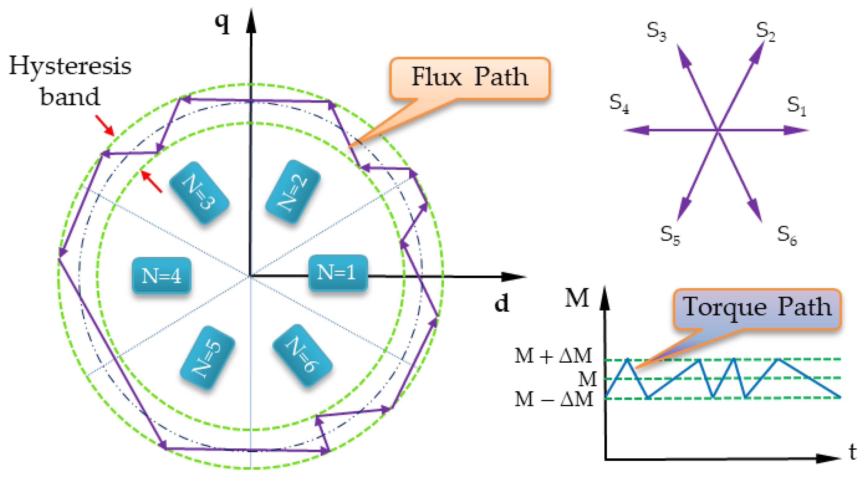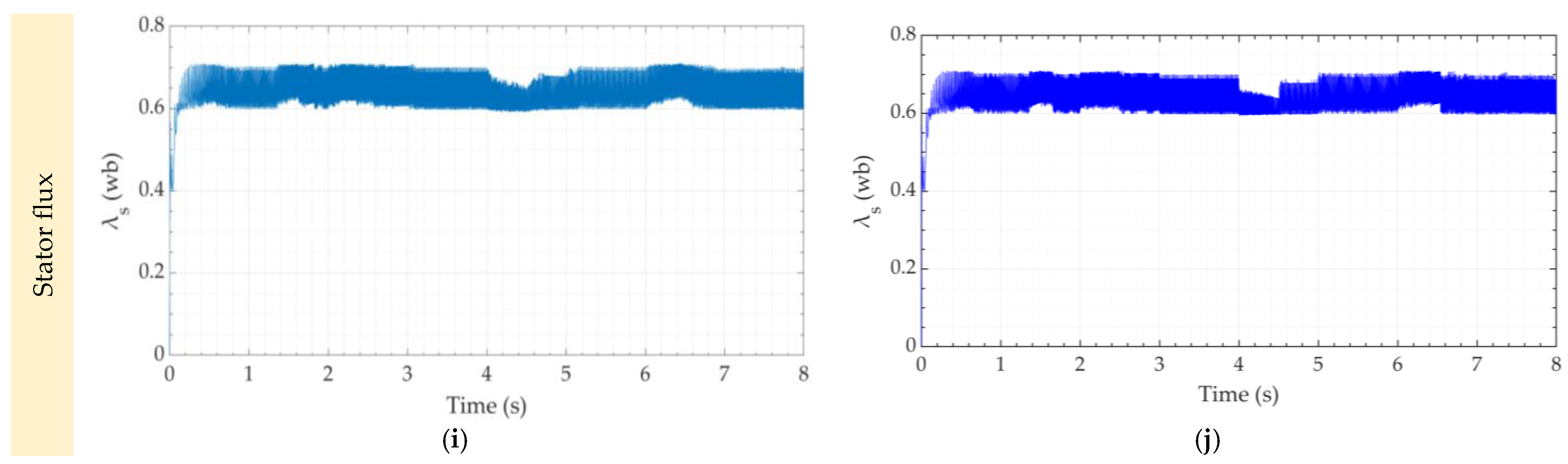Figure 8i,j also show the profile of the AM stator flux for both controllers in relation to the commanded torque produced by the speed controller. Within a hysteresis band, it is found that the magnitude of the stator flux is maintained at its full load value. This issue is crucial to have maximum torque under all conditions in the AM drive.

Some of the AM variables are changed in order to assess the strong stability of the suggested PSO-optimized FOPI regulator versus the variations of the AM parameters. There is a 10% increase in the AM rotor resistance. The AM’s speed response under parameter uncertainty is shown in Figure 9. Despite the modeling mistakes, it is found that the suggested regulator can accurately keep the speed response stable under all disturbances.

Table 7. Peak transients using both the conventional PI and the suggested optimized FOPI controllers.

Time (s)	Disturbance (%)	Highest Overshoot of ω (%)		Settling Time (s)		Steady-State Error (%)
		PSO-Optimized FOPI	Conventional PI	PSO-Optimized FOPI	Conventional PI	PSO-Optimized FOPI	Conventional PI
0	Δω = 50%, ΔMl = 100%	~0.0	~0.0	0.6	0.9	0	−0.5
1.5	ΔMl = −50%	~0.0	~0.0	0.25	0.5	0	2.5
1.38	Δω = 25%	~0.0	~0.0	~0.0	0.16	0	2.5
[2, 2.5]	dω/dt = 400 rpm/s	~0.0	~0.0	~0.0	0.1	0	−5
3	ΔMl = −50%	~0.0	~0.0	~0.0	0.2	0	−0.14
[4, 4.5]	dω/dt = −800 rpm/s	~0.0	~0.0	~0.0	0.4	0	15
5	ΔMl = 100%	~0.0	~0.0	~0.0	0.3	0	−2.5
[6, 6.5]	dω/dt = 600 rpm/s	~0.0	~0.0	0.04	0.2	−0.5	−13.5
6.5	ΔMl = −75%	~0.0	~0.0	~0.0	0.3	0	3.3

shows the evaluation of the peak overshoot for every period of the outcomes using the suggested FOPI and the traditional PI controller. With the suggested FOPI, the speed’s peak overshoot is significantly less than with the traditional PI controller for a range of load torque (M_l) and AM speed (ω) disturbances. The average improvement in the settling time is about 84.4%, and that in the steady-state error is almost killed for all disturbances using the proposed optimized FOPI controller. Also, the ITAE, given by Equation (27), has been calculated for the PI controller, during simulation, and compared to that of the optimized controller. The suggested controller provides a reduction in the cost function of about 200%.

6. Conclusions

An AM drive with direct torque control principles has been proposed in this study; nevertheless, the power converter operation has been improved to provide fast torque performance. To ensure quick torque response, an optimization study and design were conducted for the inverter operation. Optimized FOPI was used to increase the AM drive speed response. The PSO method was utilized to optimize the FOPI. MATLAB/Simulink was used to model and simulate the suggested AM drive with the optimized control system. The responses of the introduced drive utilizing the optimized FOPI, optimal PI, and the conventional PI controllers were compared. The optimal speed and torque performances are provided by the optimized FOPI controller, according to the simulation results. Comparing the proposed controller to the traditional PI, the speed errors evaluated by ITAE of the AM drive decreased by roughly 200%. Additionally, the AM’s performance with the suggested optimized FOPI under parameter uncertainties was examined. The average improvement in the settling time is about 84.4%, and that in the steady-state error is almost killed for all disturbances using the proposed optimized FOPI controller. The findings showed that the system offers reliable performance when the rotor resistance increases to 10%. Using the optimization techniques used in this study, AM drive position control will be the subject of future research. Furthermore, a crucial future consideration will be the experimental implementation of the suggested drive using the optimized FOPI controller.