BetaSigmaSlurryFoam: An Open Source Code for the Numerical Simulation of Pseudo-Homogeneous Slurry Flow in Pipes

Abstract

In this study, we present, test, and make available to the scientific community the betaSigmaSlurryFoam solver, which is a two-phase model based on the Eulerian-Eulerian approach for the simulation of turbulent slurry transport in piping systems. Specifically, betaSigmaSlurryFoam is a fully open source implementation, within the OpenFOAM platform, of the existing $\beta$-$\sigma$ two-fluid model, developed over a decade by researchers at Politecnico di Milano, which, as certified by scientific publications, proved an effective way to simulate the pipe flow of fine particle slurries in the pseudo-homogeneous regime. In this paper, we first provide the mathematical and coding details of betaSigmaSlurryFoam. Afterwards, we verify the new solver by comparison with the earlier $\beta$-$\sigma$ two-fluid model for the case of slurry transport in a horizontal pipe, demonstrating not only that the two solutions are very close to each other, but also that the effects of the two calibration coefficients $\beta$ and $\sigma$ are the same for the two implementations. Finally, we apply betaSigmaSlurryFoam to the more complex case of slurry transport in a horizontal pipe elbow, which has never been subject to investigation using the earlier $\beta$-$\sigma$ two-fluid model. We prove that the solution of betaSigmaSlurryFoam is physically consistent, and, after assessing the impact of $\beta$ and $\sigma$ through an extensive sensitivity analysis, we show that reasonably good agreement could be achieved against experimental data reported in the literature even for slightly different particle sizes than those considered in our previous research. The sharing of betaSigmaSlurryFoam as open source code promotes its further development by fostering collaboration between research groups worldwide.

1. Introduction

Pipe transport of particles in the form of slurry is a common way to convey granular material over long distances in the mining industry [1]. At the same time, slurry flows in piping systems are encountered in several other engineering applications. As a few non-exhaustive examples, we mention the conveying of particulate food materials mixed with water in the food industry [2], the use of slush nitrogen [3] or micro-encapsulated phase change material (MPCM) slurry [4] in cooling processes, the hydraulic conveying of coal ash in thermal power plants [5], and ice pigging technology, which employs a slurry of small ice crystals in a brine solution to clean pipes and ducts [6]. In order to improve the efficiency of slurry pipe transport, reducing energy and water consumption as well as operation costs, a deep understanding of the phenomena occurring in the pipe system is needed. From this perspective, numerical simulation through computational fluid dynamics (CFD) has emerged as a highly effective approach, owing to the fact that CFD provides a lot of distributed information at the local scale and, compared with laboratory testing, does not suffer from limitations in terms of size and complexity of the geometries to be investigated.

However, as we pointed out in a previous review paper [7], there are still open challenges in the CFD simulation of slurry pipe transport. The complexity of the physical processes and the wide range of space and time scales involved precludes the fully, physically-based description of the two-phase flow for reasons of excessive computational cost. Therefore, typical engineering-oriented CFD models for slurry flow rely on the Eulerian-Eulerian approach (two-fluid models), in which both phases are treated as interpenetrating continua and are solved in the Eulerian, cell-based framework. Appropriate closures and constitutive equations are required to describe the behavior of the solid phase in the Eulerian framework, hence augmenting the uncertainty of the CFD solution and enhancing the key role played by the experimental calibration and validation. Such closures and constitutive equations represent a significant modelling challenge, since they must properly represent the key physical mechanisms governing particle transport based on information above the particle scale. In turn, the transport mechanisms depend on the regime of slurry pipe flow.

As a result of a decade of research at Politecnico di Milano, with important contributions from Concentration, Heat, And Momentum (CHAM) Limited and Czech Technical University in Prague, the $\beta$-$\sigma$ two-fluid model, which allows for efficient and accurate simulation of slurry pipe flows in the pseudo-homogeneous regime [8,9,10], was developed and implemented within the PHOENICS 2018 code. The pseudo-homogeneous regime takes place when fine particles (size∼100–200 $\mathsf{\mu }$m) flow in the pipe at a velocity high enough for turbulent dispersion to be the main mechanism driving the particle transport (say above 1.5–2 m/s). Hence, the peculiar features of the $\beta$-$\sigma$ two-fluid model are the modelling of the turbulent dispersion of the particles, as well as of their interactions with the pipe wall. Conversely, neither the solid pressure nor the solid viscosity are introduced in the model, as these terms are associated with particle–particle interactions, which are negligible in pseudo-homogeneous flow.

Conversely, Eulerian-Eulerian models applicable to flow regimes in which the collisional transport plays a role, such as the heterogeneous regime, must include the viscosity and the pressure of the solid phase. These terms are typically modeled through closures derived from the Kinetic Theory of Granular Flow (KTGF), which expresses them as a function of the granular temperature, governed by an advection-diffusion-reaction equation. Nowadays, KTGF-based Eulerian-Eulerian models are very popular among academics and practitioners, as also enhanced by the availability of these models within the most widely used CFD codes. However, there are two main open challenges to be addressed.

Primarily, there is no unified model capable of simulating slurry pipe flow over different regimes. All models, in fact, have been successfully applied to specific regimes or flow conditions. As already mentioned, the $\beta$-$\sigma$ two-fluid model was used to simulate the pseudo-homogeneous flow in which the transport of fine particles is governed by turbulent dispersion. Conversely, applications of KTGF-based models have been reported mostly for situations in which locally high values of solid concentration cannot exclude an influence of particle-particle interactions. These include, for instance, the heterogeneous flow of relatively coarse particles [11,12,13], slurry flow of relatively fine particles at very high solid loading [14,15], slurry flow of small but very heavy particles [16]. Restricting the applicability of a model to a specific regime greatly limits its impact. In fact, some important technical parameters in slurry pipeline technology do not refer to a single flow regime but, rather, to the boundary between two regimes; this is the case, for instance, of the limit deposition velocity that identifies the first occurrence of particle deposit [1]. Additionally, multiple regimes (or, better, multiple transport mechanism) can co-exist in complex components of a slurry pipe system, where the interest in CFD is further enhanced.

Another unresolved issue concerns the control of the existing Eulerian-Eulerian models. As already noted, the Eulerian description of the two phases and, particularly, of the solid one, requires a number of closures and constitutive models. Although these additional equations can rely on a theoretical basis, in the end they have some empirical content, which takes the form of coefficients, sub-models, and parameters not well characterized or difficult-to-decide. The presence of these terms contribute to the overall uncertainty of the CFD solution, through a modelling uncertainty which adds to the numerical uncertainty arising from the discretization of the flow equations [7]. In order to obtain confidence in the predictions of Eulerian-Eulerian models, the modelling uncertainty must be properly controlled and, possibly, reduced, and this requires extensive sensitivity analyses, experimental calibration, and validation. In a recently published paper [10], we addressed these aspects in relation to the $\beta$-$\sigma$ two-fluid model, whose name arises precisely from the two key tuning coefficients. We clearly defined the applicability limits of the model, and we presented a sensitivity analysis aimed at assessing the role played by $\beta$ and $\sigma$ in different features of the CFD solution, which paved the way to proposing a strategy for their experimental calibration. However, to the best of our knowledge, no extensive methodological study was reported for other Eulerian-Eulerian models for the simulation of slurry transport, including KTGF-based ones. Although sensitivity analyses with respect to some features of KTGF-based Eulerian-Eulerian models have been reported in the literature, e.g., [11,15,17,18,19], it has not been well established yet as to which is the complete set of coefficients, sub-models, and parameters of this modelling framework and, among them, which deserves the most attention. This is fundamental to understanding the real predictive capacity of these models within and outside the calibration conditions, and hence their application impact.

We believe that, in addressing these challenges, sharing open source software would be of great advantage, through fostering the cooperation and collaboration of different research groups worldwide. This is in line with the open source philosophy, documented by the number of projects focused on collaborative CFD development through open source tools [20,21,22]. From this perspective, we are here presenting a fully open implementation of the $\beta$-$\sigma$ two-fluid model within the OpenFOAM platform (version 2206), which is called betaSigmaSlurryFoam, providing the complete set of subroutines as Supplementary Material accompanying this article. Specifically, the TwoPhaseEulerFoam solver was the starting point for our implementation. Note that specific routines for incorporating the KTGF closures into the TwoPhaseEulerFoam solver are available, although they were not used within the scope in the present work.

OpenFOAM is a widely used open source code in academia and industry, which includes relevant pre-implemented utilities. Some application examples of this code to slurry flow processes can be found in the literature, which strengthens our conviction that sharing the $\beta$-$\sigma$ two-fluid model through this platform might be an opportunity to foster new achievements. Shouten et al. [23,24] used the TwoPhaseEulerFoam solver with KTGF closures to simulate slurry pipe flows. In [23], these authors focused on the transport of fine particle slurry (90 $\mathsf{\mu }$m and 165 $\mathsf{\mu }$m) at high velocity (3 to 4.33 m/s), limiting the experimental validation to concentration profiles. In [24], the scope of the study was broadened, validating also the hydraulic gradient predictions and considering particle sizes up to 440 $\mathsf{\mu }$m. An interesting discussion about the importance of different types of forces acting on the particles was reported. Other publications investigated more specific features of slurry flow. Reyes and Ihle [25] studied the effect of the phase distribution on the exchange rates of different ionic species in the slurry. Mackenzie et al. [26] developed a hybrid Eulerian-Eulerian/Eulerian-Lagrangian approach to predict the slurry erosion of a square pipe bend. Liu et al. [27] investigated the pipe flow of natural gas hydrated slurry, including phase change about hydrate formation and decomposition as well as aggregation within an Eulerian-Eulerian framework. Ghoudi et al. [28] studied the transport of slurry batches in a water pipe, presenting validation of the TwoPhaseEulerFoam solver with KTGF closures against two experimentally determined concentration profiles of glass bead slurry transport in a pipe.

The objective of this work is to present, test, and share a fully open-source implementation of the previously developed $\beta$-$\sigma$ two-fluid model through the OpenFOAM platform. The goal was achieved by means of the already mentioned betaSigmaSlurryFoam solver, which, preserving the main features of the earlier $\beta$-$\sigma$ two-fluid model, integrates into and takes advantage of some OpenFOAM utilities. Hence, it was necessary to demonstrate that the new solver is consistent with the earlier one, in terms of both quantitative results and impact of the two tuning coefficients, $\beta$ and $\sigma$. Such analysis was performed by referring to the case of slurry flow in horizontal pipes, the one considered in our previous studies. Afterwards, we successfully tested the good predictive capacity of the betaSigmaSlurryFoam solver for a more complex case, which was never a subject of investigation with the $\beta$-$\sigma$ two-fluid model. This was turbulent slurry transport in a horizontal pipe bend, and reference was made to the experimental data of Kaushal et al. [29]. To the best of our knowledge, no fluid dynamic model specifically dedicated to fully suspended slurry flow is available in OpenFOAM; thus, making the well-established $\beta$-$\sigma$ two-fluid model available through the betaSigmaSlurryFoam will be of benefit to those studying this type of flow. At the same time, taking advantage of other KTGF based solvers already available on OpenFOAM, it will help researchers to achieve the long-term goal of developing a unified model for slurry transport and sediment-laden flow over different regimes.

2. Key Features of the $\mathit{\beta }$-$\mathit{\sigma }$ Two-Fluid Model

We now recall the main characteristics of the $\beta$-$\sigma$ two-fluid model in its most recent formulation. Only a brief summary is given in the next sections of this manuscript; for an exhaustive dissertation of all equations, boundary conditions, and applicability criteria, we refer the readers to our previous works [8,9].

2.1. Fluid-Dynamic Model

The $\beta$-$\sigma$ two-fluid model arose as an extension of the inter-phase slip algorithm of Spalding [30], built-in in the PHOENICS code, which incorporated some peculiar features to broaden its applicability to pseudo-homogeneous slurry pipe flow. As in all our previous works, we assumed the liquid phase to be incompressible, the process to be isothermal, and the flow to be turbulent and statistically stationary. With regard to the last feature of the flow, PHOENICS allows solving statistically stationary flows through a steady-state solver. Conversely, the betaSigmaSlurryFlow solver in OpenFOAM uses a transient solver, and characterizes the stationary state through a negligible time variation of the CFD solution. Hence, for coherence with the scope of this manuscript, the formulation of the $\beta$-$\sigma$ two-fluid model presented hereafter is the transient one, which includes the time derivative terms.

The mass and momentum conservation equations for the liquid phase (l) and the solid phase (s) are expressed as follows,

$${\displaystyle \frac{\partial {\Phi }_{\mathrm{l}}{\rho }_{\mathrm{l}}}{\partial t}}+\nabla ·\left({\Phi }_{\mathrm{l}}{\rho }_{\mathrm{l}}{\mathit{U}}_{\mathrm{l}}\right)-\nabla ·\left({\rho }_{\mathrm{l}}{\displaystyle \frac{{\mu }_{\mathrm{l}}^{\mathrm{t}}}{{\rho }_{\mathrm{l}}\sigma }}\nabla {\Phi }_{\mathrm{l}}\right)=0$$

(1)

$${\displaystyle \frac{\partial {\Phi }_{\mathrm{s}}{\rho }_{\mathrm{s}}}{\partial t}}+\nabla ·\left({\Phi }_{\mathrm{s}}{\rho }_{\mathrm{s}}{\mathit{U}}_{\mathrm{s}}\right)-\nabla ·\left({\rho }_{\mathrm{s}}{\displaystyle \frac{{\mu }_{\mathrm{l}}^{\mathrm{t}}}{{\rho }_{\mathrm{l}}\sigma }}\nabla {\Phi }_{\mathrm{s}}\right)=0$$

(2)

$$\begin{array}{cc}\hfill {\displaystyle \frac{\partial {\Phi }_{\mathrm{l}}{\rho }_{\mathrm{l}}{\mathit{U}}_{\mathrm{l}}}{\partial t}}+\nabla ·\left({\Phi }_{\mathrm{l}}{\rho }_{\mathrm{l}}{\mathit{U}}_{\mathrm{l}}{\mathit{U}}_{\mathrm{l}}\right)=-{\Phi }_{\mathrm{l}}\nabla P& +\nabla ·\left[{\Phi }_{\mathrm{l}}({\mu }_{\mathrm{l}}+{\mu }_{\mathrm{l}}^{\mathrm{t}})\nabla {\mathit{U}}_{\mathrm{l}}\right]+\hfill \\ & +{\Phi }_{\mathrm{l}}{\rho }_{\mathrm{l}}\mathbf{g}+{\mathit{M}}_{\mathrm{s}\to \mathrm{l}}+\nabla ·\left({\rho }_{\mathrm{l}}{\displaystyle \frac{{\mu }_{\mathrm{l}}^{\mathrm{t}}}{{\rho }_{\mathrm{l}}\sigma }}{\mathit{U}}_{\mathrm{l}}\nabla {\Phi }_{\mathrm{l}}\right)\hfill \end{array}$$

(3)

$$\begin{array}{cc}\hfill {\displaystyle \frac{\partial {\Phi }_{\mathrm{s}}{\rho }_{\mathrm{s}}{\mathit{U}}_{\mathrm{s}}}{\partial t}}+\nabla ·\left({\Phi }_{\mathrm{s}}{\rho }_{\mathrm{s}}{\mathit{U}}_{\mathrm{s}}{\mathit{U}}_{\mathrm{s}}\right)=-{\Phi }_{\mathrm{s}}\nabla P& +\nabla ·\left({\Phi }_{\mathrm{s}}{\mu }_{\mathrm{s}}^{\mathrm{t}}\nabla {\mathit{U}}_{\mathrm{l}}\right)+\hfill \\ & +{\Phi }_{\mathrm{s}}{\rho }_{\mathrm{s}}\mathbf{g}+{\mathit{M}}_{\mathrm{l}\to \mathrm{s}}+\nabla ·\left({\rho }_{\mathrm{s}}{\displaystyle \frac{{\mu }_{\mathrm{l}}^{\mathrm{t}}}{{\rho }_{\mathrm{l}}\sigma }}{\mathit{U}}_{\mathrm{s}}\nabla {\Phi }_{\mathrm{s}}\right)\hfill \end{array}$$

(4)

where, for each phase k = l, s, $\Phi$ is the volume fraction, $\rho$ is the density, $\mathit{U}$ is the velocity vector, and ${\mu }^{\mathrm{t}}$ is the eddy viscosity, Moreover, P is the pressure, shared by the phases, ${\mu }_{\mathrm{l}}$ is the viscosity of the liquid phase, $\mathit{g}$ is the gravitational acceleration vector, and the vectors ${\mathit{M}}_{\mathrm{s}\to \mathrm{l}}$ and ${\mathit{M}}_{\mathrm{l}\to \mathrm{s}}$, which will be discussed later, represent the action that one phase exerts on the other. Equations (1)–(4) are the essentially the basic equations of the IPSA in the transient formulation with eddy viscosity assumption, as reported in the relevant page of the PHOENICS Encyclopedia [31]. Indeed, one difference exists: the viscosity of the solid phase does not appear in Equation (4), whereas in the IPSA, ${\mu }_{\mathrm{s}}$ is set equal to ${\rho }_{\mathrm{s}}{\mu }_{\mathrm{l}}/{\rho }_{\mathrm{l}}$. This choice was made on the grounds of our previous paper [9], which demonstrated that, for fully suspended turbulent slurry transport, ${\mu }_{\mathrm{s}}$ is much smaller than ${\mu }_{\mathrm{s}}^{\mathrm{t}}$. The mathematical grounding of the two-fluid model formulation above has been explained in Messa et al. [7], where it was clarified that the variables $\Phi$, $\rho$, $\mathit{U}$, and P shall be interpreted as the time average of the locally volume averaged values. Furthermore, the last terms in Equations (1)–(4) are called phase diffusion terms, and arise from the modelling of the double correlations between the fluctuating velocities and the fluctuating volume fractions. They are a peculiar feature of the IPSA, and, in their mathematical expression, there appears the turbulent Schmidt number for volume fraction, $\sigma$, which is one of the two tuning coefficients of the $\beta$-$\sigma$ two-fluid model.

The eddy viscosity of the liquid, ${\mu }_{\mathrm{l}}^{\mathrm{t}}$, could be expressed virtually by any eddy viscosity-based turbulence model applicable within the Eulerian-Eulerian framework. However, in all our previous studies on the $\beta$-$\sigma$ two-fluid model, we have always used the two-phase extension of the high-Reynolds k-$\epsilon$ standard turbulence model of Launder and Spalding [32] available in the PHOENICS code [33]. This consists of two transport equations, one for the turbulent kinetic energy of the liquid phase, $k_{\mathrm{l}}$, and the other for its dissipation rate, ${\epsilon }_{\mathrm{l}}$, which include phase diffusion terms for consistency with the IPSA formulation. A third equation is an algebraic expression relating ${\mu }_{\mathrm{l}}^{\mathrm{t}}$, $k_{\mathrm{l}}$, and ${\epsilon }_{\mathrm{l}}$.

The already mentioned vectors ${\mathit{M}}_{\mathrm{s}\to \mathrm{l}}$ and ${\mathit{M}}_{\mathrm{l}\to \mathrm{s}}$ were here evaluated under the assumption that the drag force was the main contribution to the transfer of momentum between the two phases. Owing to the action-reaction principle, they are equal and opposite; hence, the following formula was applied:

$${\mathit{M}}_{\mathrm{l}\to \mathrm{s}}=-{\mathit{M}}_{\mathrm{s}\to \mathrm{l}}={\displaystyle \frac{{\Phi }_{\mathrm{s}}}{{\displaystyle \frac{4}{3}}\pi {\left({\displaystyle \frac{d_{\mathrm{p}}}{2}}\right)}^3}}·{\displaystyle \frac{1}{2}}{\rho }_{\mathrm{l}}\left(\pi {\displaystyle \frac{d_{\mathrm{p}}^2}{4}}\right)C_{\mathrm{d}}{U}_{\mathrm{rel}}\left({\mathit{U}}_{\mathrm{l}}-{\mathit{U}}_{\mathrm{s}}\right)$$

(5)

where $d_{\mathrm{p}}$ is the particle size, $C_{\mathrm{d}}$ is the drag coefficient acting on a particle in the slurry, and $U_{\mathrm{rel}}$ is the magnitude of the relative velocity between the two phases. The evaluation of $C_{\mathrm{d}}$ is peculiar to the $\beta$-$\sigma$ two-fluid model. Use is made of the common formula by Schiller and Naumann [34] for the drag coefficient on a single spherical particle in a uniform flow:

$$C_{\mathrm{d}}=\max \left[{\displaystyle \frac{24}{{\mathrm{Re}}_{\mathrm{m}}}}{(1+0.15{\mathrm{Re}}_{\mathrm{m}})}^{0.687},0.44\right]$$

(6)

in which the particle Reynolds number is replaced by the friction Reynolds number, ${\mathrm{Re}}_{\mathrm{m}}$, defined as:

$${\mathrm{Re}}_{\mathrm{m}}={\displaystyle \frac{{\rho }_{\mathrm{l}}{d}_{\mathrm{p}}{U}_{\mathrm{rel}}}{{\tilde{\mu }}_{\mathrm{m}}}}$$

(7)

The friction-related parameter of the slurry, ${\tilde{\mu }}_{\mathrm{m}}$, accounts for the effect of the surrounding particles on the flow resistance encountered by a single particle in the slurry. It is expressed as a function of the local solid volume fraction, ${\Phi }_{\mathrm{s}}$, as follows:

$${\tilde{\mu }}_{\mathrm{m}}={\mu }_{\mathrm{l}}\exp \left\{{\displaystyle \frac{2.5}{\beta }}\left[{\displaystyle \frac{1}{{(1-{\Phi }_{\mathrm{s}})}^{\beta }}}-1\right]\right\}$$

(8)

which, albeit its different physical meaning, is formally analogous to the formula of Cheng and Law [35] to estimate the viscosity of solid-liquid suspensions across a broad range of solid concentrations. Equation (8) depends on the dimensionless parameter $\beta$, which is the second tuning coefficient of the $\beta$-$\sigma$ two fluid model. The dependence of ${\tilde{\mu }}_{\mathrm{m}}$ on ${\Phi }_{\mathrm{s}}$ is shown in Figure 1 for different values of $\beta$ in the range commonly considered in our previous studies [10]. The influence of $\beta$ is obvious only at relative high solid volume fraction, whereas it is really mild for ${\Phi }_{\mathrm{s}}$ below about 10%.

2.2. Wall Boundary Condition for the Solid Phase

The boundary conditions used in our previous applications of the $\beta$-$\sigma$ two-fluid model were inlet, outlet, axis, and solid wall. The first three were imposed using built-in functionalities of PHOENICS, which are also typical of similar software. The same holds for the wall boundary condition of the liquid phase, which was a modified formulation of the equilibrium wall function, suitable for incorporation within the Eulerian-Eulerian framework. Instead, the wall boundary condition for the solid phase is a peculiar feature of the $\beta$-$\sigma$ two-fluid model, which required user-defined coding. Specifically, the proposed condition was developed in analogy to the log-law wall function implemented in the PHOENICS code for single-phase flow [36], and it takes the form of a relation between the solid wall shear stress, ${\tau }_{\mathrm{s}}^{\mathrm{w}}$, the solid volume fraction in the near-wall cells, ${\Phi }_{\mathrm{s}}^{\mathrm{w}}$, and the magnitude of the velocity of the solid phase parallel to the wall in the near-wall cell, ${\tilde{U}}_{\mathrm{s}}^{\mathrm{w}}$:

$${\tau }_{\mathrm{s}}^{\mathrm{w}}={\Phi }_{\mathrm{s}}^{\mathrm{w}}{\rho }_{\mathrm{s}}{s}_{\mathrm{s}}{\left({\tilde{U}}_{\mathrm{s}}^{\mathrm{w}}\right)}^2$$

(9)

where the friction coefficient $s_{\mathrm{s}}$ is obtained through the following implicit expression, that assumes a logarithmic velocity profile for the solid phase in the first grid nodes:

$$s_{\mathrm{s}}={\displaystyle \frac{{\kappa }^2}{{\ln }^2\left(E·{\mathrm{Re}}_{\mathrm{s}}^{\mathrm{w}}\sqrt{s_{\mathrm{s}}}\right)}}$$

(10)

with $\kappa$ = 0.42, the Von Karman constant; E = 8.6, the roughness parameter; and ${\mathrm{Re}}_{\mathrm{s}}^{\mathrm{w}}$ the friction wall Reynolds number of the solid phase. In turn, ${\mathrm{Re}}_{\mathrm{s}}^{\mathrm{w}}$ is given by:

$${\mathrm{Re}}_{\mathrm{s}}^{\mathrm{w}}={\displaystyle \frac{{\rho }_{\mathrm{s}}{\tilde{U}}_{\mathrm{s}}^{\mathrm{w}}\delta }{{\tilde{\mu }}_{\mathrm{s}}^{\mathrm{w}}}}$$

(11)

where $\delta$ is the distance between the center of the near-wall cells and the wall, and the friction-related parameter of the solid phase, ${\tilde{\mu }}_{\mathrm{s}}^{\mathrm{w}}$, is obtained from the following equation:

$${\tilde{\mu }}_{\mathrm{m}}^{\mathrm{w}}={\Phi }_{\mathrm{s}}^{\mathrm{w}}{\tilde{\mu }}_{\mathrm{s}}^{\mathrm{w}}+{\Phi }_{\mathrm{l}}^{\mathrm{w}}{\mu }_{\mathrm{l}}^{\mathrm{w}}$$

(12)

Through the term ${\tau }_{\mathrm{s}}^{\mathrm{w}}$, which is not included in the original IPSA, the $\beta$-$\sigma$ two-fluid model is able to account for the additional energy losses due to particle-wall collisions that characterize slurry pipe flow in comparison with the single-phase case. Further discussion around the Equations (9)–(12) here above and, more generally, around the wall boundary conditions in the $\beta$-$\sigma$ two-fluid model can be found in our previous paper [8].

2.3. Applicability Conditions

The $\beta$-$\sigma$ two-fluid model has three main applicability constraints, once again outlined in Messa and Matoušek [8]. These constraints have been mostly formulated for horizontal pipe flow, which has been the main application field of the $\beta$-$\sigma$ two-fluid model, but they could be potentially generalized to arbitrary classes of flows. An important feature of these constraints is that they can be verified a priori, before running a CFD simulation.

The first constraint is related to the wall boundary condition of the solid phase presented previously. Specifically, Equation (10) assumes the solid phase velocity to follow a logarithmic profile in the centres of the near-wall cells. This appears a valid assumption if the size of the particles is sufficiently smaller than the extension of the log-law layer of the liquid phase. Hence, accordingly, we set the constraint:

$$d_{\mathrm{p}}^{+}={\displaystyle \frac{{\rho }_{\mathrm{l}}{d}_{\mathrm{p}}{U}_{\mathrm{l}}^{\ast }}{{\mu }_{\mathrm{l}}}}<30$$

(13)

where $U_{\mathrm{l}}^{\ast }=\sqrt{{\tau }_{\mathrm{l}}^{\mathrm{w}}/{\rho }_{\mathrm{l}}}$ is the friction velocity of the liquid phase. Since Equation (13) cannot be verified a priori, as it depends on the unknown wall shear stress ${\tau }_{\mathrm{l}}^{\mathrm{w}}$, we propose to replace $d_{\mathrm{p}}^{+}$ with its estimate $d_{\mathrm{p}}^{+\mathrm{B}}$, where ${\tau }_{\mathrm{l}}^{\mathrm{w}}$ is obtained by rearranging the formula of Blasius for the friction factor of turbulent, single-phase flow in hydraulically smooth pipes [37]. After some calculations, one obtains:

$$d_{\mathrm{p}}^{+\mathrm{B}}={\displaystyle \frac{d_{\mathrm{p}}}{{\displaystyle \frac{{\mu }_{\mathrm{l}}}{{\rho }_{\mathrm{l}}{V}_{\mathrm{m}}}}{\left[0.039{\left({\displaystyle \frac{{\rho }_{\mathrm{l}}{V}_{\mathrm{m}}D}{{\mu }_{\mathrm{l}}}}\right)}^{-0.25}\right]}^{-0.5}}}$$

(14)

where $V_{\mathrm{m}}$ is the bulk velocity of the slurry, that is, the ration of the slurry volumetric flow rate and the cross section area of the pipe, and D is the pipe diameter. In practice, for a given pipe diameter and particle characteristics, Equation (13) is used to obtain the maximum transport velocity at which the $\beta$-$\sigma$ two-fluid model is applicable. Recently, we have added another constraint $d_{\mathrm{p}}^{+}\approx d_{\mathrm{p}}^{+\mathrm{B}}$ > 5, to prevent situations in which very tiny particles are transported within the viscous sub-layer, which is typical of the homogeneous regime.

The two other constraints are related to the fact that the $\beta$-$\sigma$ model assumes particle transport to be due to their interaction with the turbulent liquid, with negligible influence of particle–particle interactions. This implies, firstly, that the bulk velocity is sufficiently high compared to the limit deposition velocity, $V_{\mathrm{dl}}$, below which the particles start to form a deposit. The practical, a priori constraint takes the following form:

$$V_{\mathrm{m}}>1.5V_{\mathrm{dl}}^{\mathrm{T}}$$

(15)

where $V_{\mathrm{dl}}^{\mathrm{T}}$ is the estimate of the $V_{\mathrm{dl}}^{\mathrm{T}}$ obtained through the formula by Thomas [38], which is applicable over a wide range of flow conditions.

$$V_{\mathrm{dl}}^{\mathrm{T}}=F_{\mathrm{L}}\sqrt{2\left|\mathit{g}\right|D\left({\displaystyle \frac{{\rho }_{\mathrm{s}}}{{\rho }_{\mathrm{l}}}}-1\right)}$$

(16)

$$F_{\mathrm{L}}=2+0.305{\log }_{10}▵+1.1\times {10}^{-4}{▵}^{-0.489}-0.044{({10}^7▵)}^{-1.06}$$

(17)

$$▵={\displaystyle \frac{3}{4}}{\displaystyle \frac{{\rho }_{\mathrm{l}}{w}_{\mathrm{t}}^2}{\left|\mathit{g}\right|D({\rho }_{\mathrm{s}}-{\rho }_{\mathrm{l}})}}$$

(18)

where $w_{\mathrm{t}}$ is the settling velocity of a single spherical particle in a fluid, which depends on the drag coefficient, and can be easily obtained in an iterative manner. The third and last constraint sets an upper limit to the local solid volume fraction, ${\Phi }_{\mathrm{s}}$ which must be below 0.45. The underlying concept is that, if the solid concentration is very high, particle–particle interactions might play an important role, even at high velocity. The upper threshold value of 0.45 was obtained from the experimental study by Korving [39], who detected a sudden increase in hydraulic gradient above this concentration level, even at transport velocities well above the limit deposition value. Since the fulfillment of the condition ${\Phi }_{\mathrm{s}}$ can be verified only a posteriori, we changed the constraint into $C_{\mathrm{in}}$ < 0.40, where $C_{\mathrm{in}}$ is the area-averaged solid volume fraction at the inlet section of the pipe.

3. Key Implementation Details of betaSigmaSlurryFoam

As anticipated, betaSigmaSlurryFoam, which is the OpenFOAM implementation of the $\beta$-$\sigma$ two-fluid model, was developed starting from the twoPhaseEulerFoam solver and making the necessary modifications. Specifically, our main tasks were to include the phase diffusion terms in all conservation equations, to define the drag coefficient as a function of the friction parameter ${\tilde{\mu }}_{\mathrm{m}}$, and to implement the wall boundary condition for the solid phase, which also depends on the variable ${\tilde{\mu }}_{\mathrm{m}}$.

Only the key aspects of twoPhaseEulerFoam will be recalled here, since a detailed description of the algorithms is out of the scope of this manuscript and, in this context, we refer the interested readers to the documentation of OpenFOAM. TwoPhaseEulerFoam uses the transient PIMPLE method for pressure-velocity coupling. In twoPhaseEulerFoam, at every calculation time, the five steps illustrated in the flow chart in Figure 2 are executed sequentially. The inclusion of the phase diffusion terms affected all five steps, requiring the modification of several scripts. Note that phase diffusion terms were included not only in the mass and momentum conservation equations, but also in the transport equations of the turbulence model for the liquid phase. In this study, we used two turbulence models, namely, the k-$ϵ$ standard turbulence model, employed in the straight pipe flow simulations for coherence with our previous studies with the $\beta$-$\sigma$ two-fluid model, and the k-$\omega$ SST turbulence model, selected for the analysis of the slurry transport in the pipe bend based on a previous investigation in single-phase conditions [40]. Hence, the subroutines of these two turbulence models also had to be customized. The introduction of the friction parameter ${\tilde{\mu }}_{\mathrm{m}}$ was made in a dedicated code block between step 1 and step 2. After step 1, the volume fraction of the solid phase at the current time, ${\Phi }_{\mathrm{s}}$, was obtained. This was used to calculate ${\tilde{\mu }}_{\mathrm{m}}$ and, in cascade, the friction Reynolds number, ${\mathrm{Re}}_{\mathrm{m}}$, and the drag coefficient, $C_{\mathrm{d}}$, through Equations (8), (7) and (6), respectively. At this point, the interfacial momentum transfer vectors, ${\mathit{M}}_{\mathrm{l}\to \mathrm{s}}$ and ${\mathit{M}}_{\mathrm{s}\to \mathrm{l}}$ were calculated through Equation (5), and these became part of the phase velocity predictor equations, which are step 2 in the solution algorithm. The wall boundary condition of the solid phase was implemented similarly to the PHOENICS code. Specifically, a vector source term was added to the finite volume formulation of the solid phase momentum equation in all near-wall cells, with the following form:

$${\mathbf{S}}_{\mathrm{s}}^{\mathrm{w}}=-{\Phi }_{\mathrm{s}}^{\mathrm{w}}{\rho }_{\mathrm{s}}{s}_{\mathrm{s}}{A}^{\mathrm{w}}{\tilde{U}}_{\mathrm{s}}^{\mathrm{w}}{\mathit{U}}_{\mathrm{s}}^{\mathrm{w}}$$

(19)

where $A^{\mathrm{w}}$ is the area of the near-wall cell, ${\mathit{U}}_{\mathrm{s}}^{\mathrm{w}}$ is the solid velocity vector in the near-wall cell, and, as already mentioned, ${\tilde{U}}_{\mathrm{s}}^{\mathrm{w}}$ is the magnitude of the solid phase velocity parallel to the wall in the near-wall cell. Equation (19) can be seen as a generalization of Equation (9), suitable for inclusion within a 3D framework, in which there exist two velocity components parallel to the wall, and one velocity component normal to it. The friction coefficient, $s_{\mathrm{s}}$, is obtained from Equations (10)–(12), and Equation (10) could be solved in six iterations with a satisfactory degree of accuracy.

Although the model equations are basically the same, some inherent differences exist between the formulation of the $\beta$-$\sigma$ in PHOENICS and betaSigmaSlurryFoam. One concerns the implementation of the wall boundary condition of the liquid phase. In fact, PHOENICS incorporates in the momentum equations of the liquid phase a source term analogous to Equation (19), with some small differences in the evaluation of the friction coefficient. Conversely, the most straightforward option in OpenFOAM is to call dedicated WallFunction subroutines, e.g., nutkWallFunction, nutkRoughWallFunction, kqRWallFunction, epsilonWallFunction, and omegaWallFunction. Preliminary tests performed for single-phase flow in straight pipes and channels revealed negligible differences between the PHOENICS and OpenFOAM implementations; hence, in betaSigmaSlurryFoam, we decided to adopt the built-in wall functions. Additionally, all previous applications of the $\beta$-$\sigma$ model in PHOENICS concerned the case of slurry flow in a horizontal pipe, which was discretized using a structured mesh in cylindrical-polar coordinate system. The equation formulation was elliptic-staggered, with the scalar variables stored at the cell centres and the velocity components over the cell faces. In this work, co-located grid arrangement was employed, in which all variables are stored at the cell centres. In order to ensure sufficient accuracy, most solution settings were set as those of configuration 2 in Passalacqua and Fox [41]. Specifically, for discretizing convective terms, the second-order central differencing scheme with the limiter proposed by Sweby [42] was used. A special version of this scheme, known as “limitedLinearV”, was employed for all vector terms. The second-order “Gauss vanLeer” scheme was used to discretize the term related to the volume fraction. Other terms, such as phase diffusion flux, gradient terms, and the stress tensor, were discretized using the “Gauss linear” scheme. For implicit time discretization, the first-order “Euler” scheme was employed. The other settings were left as the default ones in OpenFOAM.

The routines of the betaSigmaSlurryFoam solver are provided in a dedicated GitHub repository, indicated in the “Data Avilability Statement” section at the end of the manuscript.

4. Testing of betaSigmaSlurryFoam

The betaSigmaSlurryFoam solver was extensively tested with a two-fold objective. Firstly, the accuracy of the new implementation was verified with respect to the earlier PHOENICS solver and, for this purpose, reference was made to the case of slurry transport in a horizontal pipe considered in our previous papers. Secondly, betaSigmaSlurryFoam was employed to study a more complex flow configuration that we had never investigated before, which is slurry transport in a horizontal pipe bend, showing satisfactory predictive capacity even beyond its original application limits. The two application cases are presented in Section 4.1 and Section 4.2, respectively.

4.1. Similarity Assessment Against the Previous $\beta$-$\sigma$ Two-Fluid Model for Horizontal Pipe Flow

The good performance of the $\beta$-$\sigma$ two-fluid model for simulating the horizontal pipeline transport of fine particle slurry in the pseudo-homogeneous regime has been widely investigated in many of our previous papers. For instance, in [8], we considered three experimental datasets reported in the literature and, after exploring the influence of $\beta$ and $\sigma$ on hydraulic gradient and solid concentration profile, we made an assessment of the model accuracy and inspected difficult-to-measure quantities. In a more recent paper [10], we delved further into the role played by $\beta$ and $\sigma$ by considering different features of the CFD solution for a wider range of flow conditions (pipe diameter, inlet concentration, flow velocity); then, we developed a calibration strategy to find out suitable values of the two coefficients, and tested them against three other experimental datasets. Here, our goal was to demonstrate the consistency between betaSigmaSlurryFoam (in OpenFOAM) and the $\beta$-$\sigma$ two-fluid model (in PHOENICS), which required assessing not only that the two solvers provide very close results, but also that they are able to capture the same effects as $\beta$ and $\sigma$. Once the similarity of the two solvers was proven, presenting further experimental validation results for betaSigmaSlurryFoam would not have added significant value, given the extensive experimental assessment already reported for the $\beta$-$\sigma$ two-fluid model. In order to guarantee that the consistency of the findings was not limited to special flow conditions, the analysis was mainly focused on two extreme testing conditions among the six considered previously in [10], which were referred to as C1 (small diameter, low velocity, low concentration) and C6 (large diameter, high velocity, high concentration), and are summarized in

Table 1. Test conditions for similarity assessment based on the horizontal pipe simulations.

Simulation ID	D [mm]	${\mathit{V}}_{\mathbf{m}}$ [m/s]	${\mathit{C}}_{\mathbf{in}}$ [−]	${\mathit{\rho }}_{\mathbf{p}}$ [kg/m3]	${\mathit{d}}_{\mathbf{p}}$ [$\mathsf{\mu }$m]	${\mathit{H}}_{\mathbf{s}}$ [$\mathsf{\mu }$m]
C1	50	2.0	0.05	2650	150	0
C6	500	4.5	0.40	2650	150	0

. The symbol $H_{\mathrm{s}}$ denotes the surface roughness, assumed null in both test conditions. The range of pipe diameters defined in [10], fully covered in Table 1, was selected by considering the typical values at which experimental data were available, e.g., [43]. The upper concentration level, equal to 0.40, was dictated by one of the applicability constraints of the $\beta$-$\sigma$ two-fluid model, previously recalled in Section 2.3, whereas the lower one was regarded as well representative of slurry transport processes at moderate solid loading. For each pipe diameter, the range of flow velocity was decided by accounting for the first two applicability constraints in Section 2.3. Specifically, for D = 50 mm, we analyzed two velocities (2.0 m/s and 4.5 m/s), whereas, for D = 500 mm, we considered only the upper one (4.5 m/s), because the limit deposition velocity predicted by the formula of Thomas [38] was quite large. This was the origin of the six combinations investigated in [10], but, as already mentioned, the results will be here shown only for cases C1 and C6.

4.1.1. Numerical Set-Up

In these simulations, the turbulence model was the k-$\epsilon$ standard one to allow for consistency with our previous PHOENICS results. The domain of the horizontal pipe case was a simple cylindrical volume, in which the two end faces were the inlet and the outlet boundaries, whereas the later surface was a solid wall, as shown in Figure 3a. At the inlet boundary, uniform distributions were set to both the axial velocities of the two phases, $U_{\mathrm{l}}^{\mathrm{in}}$ = $U_{\mathrm{s}}^{\mathrm{in}}$ = $V_{\mathrm{m}}$, to the solid concentrations, ${\Phi }_{\mathrm{s}}^{\mathrm{in}}$ = 1 −${\Phi }_{\mathrm{l}}^{\mathrm{in}}$ = $C_{\mathrm{in}}$, as well as to the turbulent kinetic energy of the liquid and its dissipation rate. Note that no slip was allowed between the phases at the inlet, but both velocities were set equal to the viscosity of the mixture. At the outlet, the pressure and the normal gradient of all solved variables were set to zero. At the pipe wall, the wall shear stress of the liquid phase, as well as the turbulent kinetic energy and its dissipation rate in the near wall cells, were obtained through the built-in subroutines nutkWallFunction (since the pipe was assumed hydraulically smooth), kqRWallFunction, and epsilonWallFunction, respectively. The wall shear stress of the solid phase was evaluated through the source term in Equation (19), as explained previously. The domain was discretized using a O-type structured mesh, composed of hexahedral blocks, to reduce the computational effort and promote the numerical stability. The O-type mesh pattern was selected as it appeared a straightforward option to discretize a cylindrical pipe in OpenFOAM, as was also suggested by the previous studies on slurry pipe transport using this code [23,24,27,28]. This marks a difference with the earlier $\beta$-$\sigma$ two-fluid model in PHOENICS, where the grid was a cylindrical polar one with axis conditions. Representative pictures of the used O-type meshes are shown in Figure 3b, and a discussion around the grid independence study will be given in Section 4.1.2. Unlike the $\beta$-$\sigma$ two-fluid model in PHOENICS, betaSigmaSlurryModel is a transient solver, and hence a time discretization must be provided. The initial time step was set to as 0.002 s, and then automatically adjusted to produce a Courant number of 0.8.

4.1.2. Control of the Numerical Sources of Uncertainty

The attainment of statistically steady, fully developed flow was ensured for both cases, with $\beta$ = 2.5 and $\sigma$ = 0.75. This was achieved, firstly, by inspecting the time histories of relevant fluid dynamic parameters at some monitoring probes. The target parameters were the chord-average solid volume fraction, ${\langle {\Phi }_{\mathrm{s}}\rangle }_{\gamma }$, the axial velocity of the liquid phase, $U_{\mathrm{l},z}$, the eddy viscosity of the liquid phase, ${\nu }_{\mathrm{l}}^{\mathrm{t}}$, as well as the turbulent kinetic energy and the dissipation rate of the same phase, $k_{\mathrm{l}}$ and ${\epsilon }_{\mathrm{l}}$. By way of example, Figure 4a shows the time histories of the chord-averaged solid concentration, ${\langle {\Phi }_{\mathrm{s}}\rangle }_{\gamma }$, and of the eddy viscosity of the liquid phase, ${\nu }_{\mathrm{l}}^{\mathrm{t}}$, at the center (y = D/2) of the pipe outlet, normalized by the values after 10 s. The curves clearly indicate that, after about 5 s, statistically steady flow conditions are reached at the outlet, and hence over the entire pipe. Therefore, the physical time simulated was 5 s, and the solution was inspected at the final time instant. In order to identify fully developed flow, we increased the length of the pipe to 200D and inspected the space variation of the same fluid dynamic parameters ${\langle {\Phi }_{\mathrm{s}}\rangle }_{\gamma }$ and ${\nu }_{\mathrm{l}}^{\mathrm{t}}$ along the streamwise coordinate, z. By way of example, Figure 4b shows the streamwise profiles of ${\langle {\Phi }_{\mathrm{s}}\rangle }_{\gamma }$ (values on the left vertical axis) and ${\nu }_{\mathrm{l}}^{\mathrm{t}}$ (values on the right vertical axis) at two elevations along the vertical diameter, namely, elevation A ($y/D$ = 0.25) and elevation B ($y/D$ = 0.75). Like Figure 4a, Figure 4b is also presented in dimensionless form, with the streamwise coordinate, z, normalized by the pipe diameter, $bD$, and ${\langle {\Phi }_{\mathrm{s}}\rangle }_{\gamma }$ and ${\nu }_{\mathrm{l}}^{\mathrm{t}}$ normalized by the corresponding values at the same elevation at the pipe outlet, $z/D$ = 200. It is immediately evident that all curves in Figure 4b approach a unit value, indicating the attainment of fully developed flow conditions. A close quantitative look reveals that, at $z/D$ = 120, the values of ${\langle {\Phi }_{\mathrm{s}}\rangle }_{\gamma }$ and ${\nu }_{\mathrm{l}}^{\mathrm{t}}$ deviate by much less than 1% than the values at $z/D$ = 200. Hence, it could be reasonably argued that the solution at $z/D$ = 120 was representative of the fully developed state. However, to lie even further on the safe side and considering the low computational burden of the straight pipe simulations, the length of the computational domain was set to 150D, and the solution was inspected at the outlet section. Although no streamwise pressure profile is shown here in order to avoid making this paper too lengthy, our results indicated that the pressure started decreasing linearly almost immediately starting from the inlet boundary. In this study, the hydraulic gradient was evaluated by referring to the area-average pressures at locations 120D and 150D; however, the estimates would be indistinguishable if two different pipe sections or the pressures at the pipe axis instead of the area-averaged values were considered.

Afterwards, a sensitivity analysis with respect to the computational mesh was performed, once again for both cases and $\beta$ = 2.5 and $\sigma$ = 0.75. The study was conducted in two steps. Initially, the overall number of cells was varied, producing the four O-meshes sketched in Figure 3, keeping the distance between the center of the near-wall cells and the wall approximately equal to 30 wall units (that is, $y^{+}\approx 30$, where $y^{+}$ was calculated with respect to the friction velocity of the fluid phase). The details of the meshes are given in

Table 2. Number of cells in the four O-type meshes, sketched in Figure 3, for the horizontal pipe simulations. The last two columns are the predicted hydraulic gradients with $y^{+}$ of the near-wall cells around 30 for case C1, and the percentage deviation from the mesh 4 solution.

Mesh ID	${\mathit{N}}_{\square }$	${\mathit{N}}_{\mathbf{\Gamma }}$	${\mathit{N}}_{\mathit{z}}$	${\mathit{N}}_{\mathbf{tot}}$	${\mathit{i}}_{\mathbf{m}}$	$\mathit{▵}{\mathit{i}}_{\mathbf{m}}$
mesh1	6	6	90	16,200	0.1251	1.790%
mesh2	8	8	110	35,200	0.1237	0.651%
mesh3	10	10	130	65,000	0.1231	0.163%
mesh4	16	14	180	207,360	0.1229	-

, where $N_{\square }$ is the number of subdivisions of the edges of the central square, $N_{\Gamma }$ is the number layers of the outer ring, $N_{\mathrm{z}}$ is the number of subdivisions along the pipe axis, and $N_{\mathrm{tot}}$ is the total number of cells. The number of subdivisions was defined progressively after inspecting their effect on relevant target parameters, without the need to use specific utilities for the automatic optimization of the mesh resolution. As target parameters, the vertical profiles of the same variables mentioned before were considered, namely, ${\langle {\Phi }_{\mathrm{s}}\rangle }_{\gamma }$, $U_{\mathrm{l},z}$, ${\nu }_{\mathrm{l}}^{\mathrm{t}}$, $k_{\mathrm{l}}$, and ${\epsilon }_{\mathrm{l}}$, in addition to the hydraulic gradient, $i_{\mathrm{m}}$. For all of them, the effect of the mesh was relatively mild, as exemplified in Figure 5 ${\langle {\Phi }_{\mathrm{s}}\rangle }_{\gamma }$ and ${\nu }_{\mathrm{l}}^{\mathrm{t}}$, and in the last two columns of Table 2 for $i_{\mathrm{m}}$. Particularly, the difference between the mesh 3 and mesh 4 solutions was very small and, considering that the run time of the mesh 3 simulations was just about about 10 min on our workstation with a Xeon Gold 6248R @ 3.00 GHz (X2) processor and 256 GB RAM, using 40 cores, we decided to adopt this level of discretization.

As a second step, keeping the overall discretization as in mesh 3, the thickness of the near wall layer was varied. In one of our previous studies [9], we found that the hydraulic gradient predicted by the $\beta$-$\sigma$ two-fluid model was affected by the dimensionless wall distance of the first grid nodes, $y^{+}$, and that the influence of $y^{+}$ depends on the flow conditions, and, especially, the level of solid concentration, $C_{\mathrm{in}}$. The betaSigmaSlurryFoam was found to preserve this feature of the $\beta$-$\sigma$ two-fluid model, in spite of the different implementation of the wall boundary conditions of the liquid phase. This is shown in Figure 6 for cases C1 and C6, but similar findings were obtained also for the four other combinations of pipe diameter, bulk velocity, and inlet concentration in [10]. Hence, for the definition of the near-wall mesh, we adopted the same recommendation developed for the $\beta$-$\sigma$ two-fluid model, that is, to keep $y^{+}$ around 30, which is the smallest possible value consistent with the wall boundary condition of the liquid phase.

4.1.3. Results

The correct implementation of the betaSigmaSlurryFoam was verified against the results of the $\beta$-$\sigma$ two-fluid model obtained with the PHOENICS code and presented in our previous paper [10]. The comparison was made in terms of hydraulic gradient, chord average concentration profile, streamwise velocity profile of the two phases along the vertical diameter, and distribution of the wall shear stresses of the two phases over the pipe circumference. Here, we will show only the results for hydraulic gradient and chord average concentration profile. The axial velocity distributions, in fact, were practically insensitive to the values of $\beta$ and $\sigma$. Conversely, an effect of the two coefficients was detected on the wall shear stresses profiles, which could be interpreted mostly from the distributions of the volume fractions in the near-wall cells. In any case, for all these additional variables, there was full consistency between OpenFOAM and PHOENICS. The hydraulic gradient predictions are summarized in

Table 3. Effects of $\beta$ and $\sigma$ on the hydraulic gradient for testing conditions C1 and C6.

		betaSigmaSlurryFoam		$\mathit{\beta }$-$\mathit{\sigma }$ Model
		(OpenFOAM)		(PHOENICS)
$\mathit{\beta }$	$\mathit{\sigma }$	C1	C6	C1	C6
0.5	0.75	0.0766	0.0402	0.0801	0.0396
1.5		0.0776	0.0443	0.0802	0.0435
2.5		0.0776	0.0519	0.0803	0.0514
3.5		0.0776	0.0698	0.0805	0.0712
2.5	0.50	0.0766	0.0525	0.0789	0.0514
	0.75	0.0776	0.0519	0.0803	0.0514
	1.00	0.0786	0.0517	0.0818	0.0513

. The $i_m$ values obtained by the two solvers are reasonably similar to each other, the maximum deviation being of the order of a few percent in the C1 case. A similar situation is found when inspecting the chord-average concentration profiles, shown in Figure 7, where the biggest deviations are found close to the pipe bottom for the C1 case. The definitive identification of the reasons for the lack of a complete match between the two solutions would be very challenging, since there are peculiarities in the internal structures of the two platforms, of which the users have little or no awareness nor control capacity. At this stage, we can make only reasonable speculations based on the differences that appear immediately evident, which concern the treatments of the wall boundary condition of the liquid phase, the structure of the grid, and the post-processing techniques for extracting the chord-average concentration profile. However, the key finding is that betaSigmaSlurryFoam predicts the same influence of $\beta$ and $\sigma$ as the $\beta$-$\sigma$ two-fluid model in PHOENICS, both qualitatively and quantitatively. Specifically, changing $\beta$ has very little or no influence on the C1 solution, whereas changing $\sigma$ affects the concentration profile, with some minor effect also on the hydraulic gradient. The situation is the opposite for case C6: here, in fact, the effect of $\beta$ is obvious on both the hydraulic gradient and the concentration profile, whereas the influence of $\sigma$ is more moderate. These findings suggest that the calibration strategy of $\beta$ and $\sigma$ presented in [10] for the $\beta$-$\sigma$ two-fluid model is a valid recommendation also for the simulations performed with betaSigmaSlurryFoam. Based on the above results, the implementation of betaSigmaSlurryFoam was succesfully tested, opening the way to the testing of the new solver against a more complex case study never addressed with the $\beta$-$\sigma$ two-fluid model. We remark that, in order to strengthen our confidence in the new betaSigmaSlurryFoam solver, the similarity assessment was extended to other combinations of pipe diameter, inlet concentration, and flow velocity in [10], always obtaining full consistency with the earlier $\beta$-$\sigma$ two-fluid model in PHOENICS. Additionally, we tested betaSigmaSlurryFoam against data of hydraulic gradient and concentration profile from the same horizontal pipe experiments considered in our previous validation of the $\beta$-$\sigma$ two-fluid model [8,10]. Not surprisingly, we detected a satisfactory degree of agreement with the experimental data upon proper calibration of $\beta$ and $\sigma$, which is a reasonably accurate prediction of the slope of the concentration profile and estimates of the hydraulic gradient within $\pm 15\%$ accuracy. None of these expected results are reported in the present manuscript, as it would not have added significant value.

4.2. Validation Against Slurry Flow Experiments in a Horizontal Pipe Bend

The second test case concerns the slurry transport in a horizontal 90° pipe bend. The goal was to assess the ability of the betaSigmaSlurryFoam solver to correctly predict the behavior of a flow which is considerably more complex of that in a straight pipe, yet of engineering relevance. Particular attention was paid, once again, to the effect of $\beta$ and $\sigma$, and a comparison against data from the literature was made.

4.2.1. Description of the Test Case

The testing conditions were sourced from the experiments conducted by Kaushal et al. [29] on slurry pipe flows of silica sand in a pipeline of diameter 53 mm with 90° bends having different ratios of bend radius, $R_{\mathrm{b}}$, to pipe radius, R. Specifically, we selected the value $R_{\mathrm{b}}/R$ = 5.6, for which detailed two-phase flow data are available. The relative roughness of the pipe, $H_{\mathrm{s}}/D$, was declared as 0.0003. These experiments involved three flow velocities ($V_{\mathrm{m}}$ = 1.78 m/s, 2.67 m/s, 3.56 m/s) and three in situ concentrations ($C_{\mathrm{in}}$ = 0.0394, 0.0882, 0.1628). The granular material was silica sand with density 2650 kg/m³ and particle size 450 $\mathsf{\mu }$m. Although the particle size was larger than the typical particles used in the $\beta$-$\sigma$ two-fluid model, which are in the range 100–200 $\mathsf{\mu }$m, the authors reported critical deposition velocities around 1.55 m/s. Conservatively, we considered only the highest flow velocity (3.56 m/s), to have confidence that the slurry transport is mainly driven by particle–turbulence interaction, although it cannot be excluded that some particle–particle interactions take place within the bend or downstream of it. For every combination of slurry velocity and concentration, the authors measured the pressure at different locations upstream and downstream of the bends, by averaging the data for the inner and outer sides. They also provided vertical concentration profiles at locations 5D, 25D, and 50D downstream of the bend, using sampling probes.

4.2.2. Numerical Set-Up

The k-$\omega$ SST turbulence model was used, which, according to our previous study [40], proved effective to simulate the single-phase flow in a pipe bend. The computational domain, shown in Figure 8a, comprises the 90° bend and two straight pipes, located upstream and downstream. Their lengths were 100D and 140D, to ensure that fully developed flow is attained at the bend entrance and that a complete flow recovery has occurred before the outlet. The boundary conditions were as in the horizontal pipe case, namely, inlet, outlet, and solid walls. Once again in analogy to the previous case, uniform distributions were set for all variables, namely, the axial velocity of both phases (equal to $V_{\mathrm{m}}$), the volume fractions, the turbulent kinetic energy of the liquid phase and, as required by the k-$\omega$ SST turbulence model, the specific rate of turbulence dissipation of the liquid phase. Specifically, four test cases were considered, corresponding to the four levels of $C_{\mathrm{in}}$ (0.0394, 0.0882, 0.1628, plus the single phase case), at the velocity $V_{\mathrm{m}}$ = 3.56 m/s. The properties of the solid particles were set as detailed in Section 4.2.1. In order to account for the wall roughness, the wall shear stress of the liquid phase was obtained through the subroutine nutkRoughWallFunction, setting a sand grain roughness equal to 0.0003 times the pipe diameter. The subroutines kqRwallfunction and omegaWallFunction were used to impose the wall boundary conditions on $k_{\mathrm{l}}$ and ${\omega }_{\mathrm{l}}$, respectively. The CFD domain was discretized using a O-type mesh. The discretization pattern of the pipe cross-section was qualitatively similar to that of the straight pipe case, previously shown in Figure 3b. The size of the subdivisions along the main flow direction was smaller in the bend zone and larger in the upstream and downstream pipe; by way of example, Figure 8b shows a side view of the bend zone for “mesh 3”. As for the straight pipe case, the time step was automatically adjusted by the solver to produce a Courant number of 0.8, starting from an initial value of 0.002.

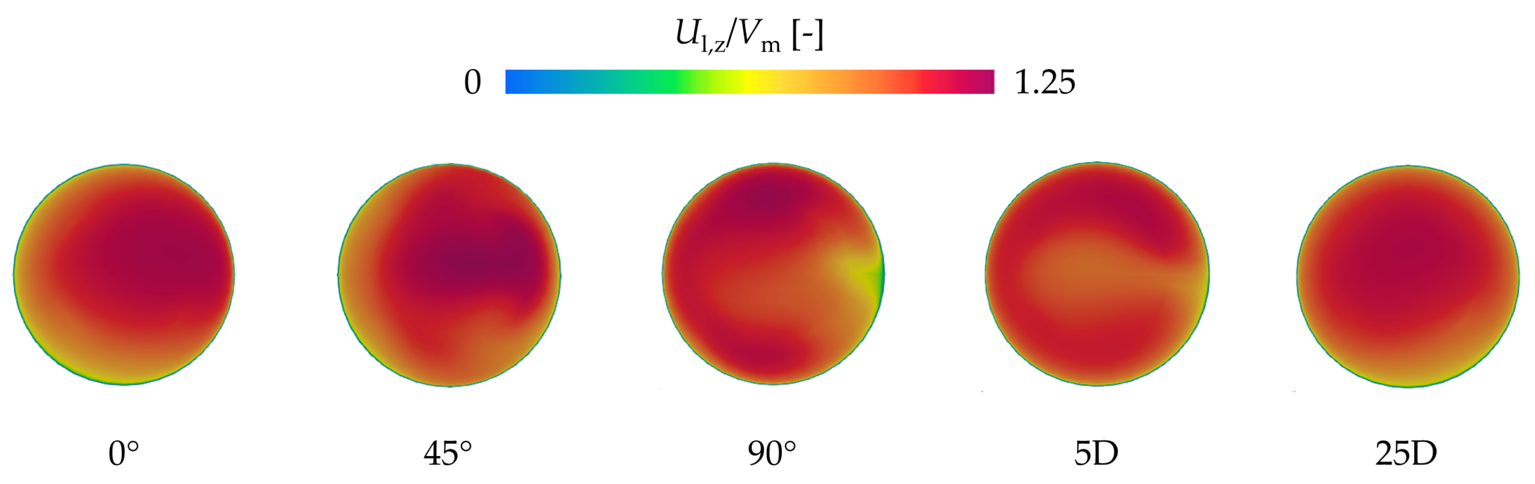
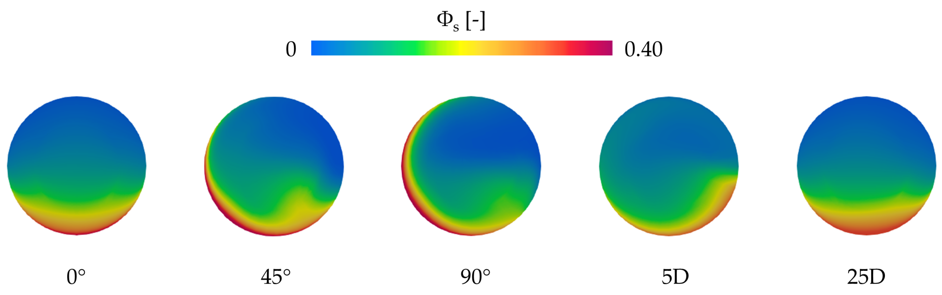
4.2.3. Inspection of the CFD Results and Their Physical Interpretation

Firstly, a qualitative assessment of the goodness of the CFD solution was carried out by interpreting the results in the light of the theoretical and physical principles. The analysis was carried out for $C_{\mathrm{in}}$ = 0.0882. The results presented hereafter refer to $\beta$ = 0.5 and $\sigma$ = 0.5, and they have been calculated using “mesh 3”.

From a qualitative point of view, the two-phase results were in line with the single-phase ones subject to investigation in our previous work [40]. Unlike in the straight pipe case, the pressure was not linearly varied with the vertical elevation in each cross section; it exhibited a more complex pattern because of the centrifugal effect of the bend. The trend of the pressure along the streamwise coordinate was quantified by the dimensionless wall pressure coefficient, defined as:

$$C_{\mathrm{p}}^{\mathrm{w}}\left(\theta ,z\right)={\displaystyle \frac{P^{\mathrm{w}}\left(\theta ,z\right)-P_{\mathrm{ref}}}{\frac{1}{2}\rho V_{\mathrm{m}}^2}}$$

(20)

where $P_{\mathrm{ref}}$ is a reference value, which was here set as the value at the intrados ($\theta$ = 0°) of the cross-section located 8D downstream of the bend exit. Figure 9 shows the curves $C_{\mathrm{p}}^{\mathrm{w}}$ versus z for two azimuthal locations, namely, the intrados and the extrados. Clearly, far upstream and far downstream of the bend, $C_{\mathrm{p}}^{\mathrm{w}}$ decreases linearly with z as a result of the major losses in the straight pipes. Between about 2D upstream and about 2D downstream of the bend, the centrifugal acceleration produces a transversal pressure gradient directed from the extrados to the intrados, which, in turn, has an impact on the velocity field.

The contours of the streamwise velocity of the liquid phase, $U_{z,\mathrm{l}}$, are shown in Figure 10 over five cross-sections at different locations along the pipe. The last section, 25D downstream of the bend exit, is essentially representative of the fully developed condition, with symmetrical behavior with respect to the vertical diameter and the point of maximum velocity in the upper half of the pipe. Inside of the bend, the point of maximum streamwise velocity first moves towards the intrados in the first half of the bend, whereas, at the exit of the bend, the region with maximum streamwise velocity is located close to the extrados. The distortion in the streamwise velocity distribution is accompanied by secondary flow. As shown in Figure 11, the secondary flow is characterized by two visible rotational structures, and changes direction from section to section. The behavior of the secondary flow, which is already quite complex in the single-phase case, is even more challenging to understand in the slurry flow case, owing to the presence of two phases interacting with each other. In order to capture in a more direct manner the secondary flow, we referred to the intensity of the secondary flow of the liquid phase, $I_{\mathrm{s},\mathrm{l}}$, defined as:

$$I_{\mathrm{s},\mathrm{l}}\left(z\right)={\displaystyle \frac{4}{\pi D^2{V}_{\mathrm{m}}^2}}{\int }_0^{2\pi }{\int }_0^R\left(U_{\theta ,\mathrm{l}}^2+U_{r,\mathrm{l}}^2\right)rdrd\theta$$

(21)

The trend $I_{\mathrm{s},\mathrm{l}}$ versus z, shown in Figure 12a, indicates that, practically speaking, the secondary flow generates starting from the entrance of the bend, and then grows, reaching the maximum value in the second half of the bend (between 45° and 90°); afterwards, it vanishes slowly, coming to almost complete suppression at a distance of about 10D downstream of the bend exit. The $I_{\mathrm{s},\mathrm{l}}$ curve is fully coherent with the secondary flow patterns depicted in Figure 11, where the length scale of the vectors is the same at all locations. Specifically, the longest vectors are seen at sections 45° and 90°, where the secondary flow had the maximum intensity. At location 25D, no vectors are visible in Figure 11, since the secondary flow had already reached complete suppression. Another cross-section averaged parameter was considered to obtain a more comprehensive picture of the liquid velocity field, namely, the turbulent energy parameter, $k_{\mathrm{a},\mathrm{l}}$:

$$k_{\mathrm{a},\mathrm{l}}\left(s\right)={\displaystyle \frac{4}{\pi D^2{V}_{\mathrm{m}}^2}}{\int }_0^{2\pi }{\int }_0^R{k}_{\mathrm{l}}rdrd\theta$$

(22)

The streamwise profile of $k_{\mathrm{a},\mathrm{l}}$, shown in Figure 12b, highlights the significant amount of turbulence produced within the bend, which is progressively dissipated in the downstream pipe and followed by a mild recovery.

The behavior of the solid particles was inspected by referring to the solid phase velocity and the local solid volume fraction. As far as the former is concerned, Figure 13 shows the contours of the magnitude of the relative velocity, $U_{\mathrm{rel}}$. The predominance of the blue color indicates that, despite their relatively large size, the 0.45 mm particles basically tend to follow the carrier liquid, even if higher slip velocities are seen within the bend, specifically on the 45° section close to the intrados. Note that this region is also characterized by strong secondary flow. The solid volume fraction distribution, provided in Figure 14, indicates that the particles are mainly likely to travel in the lower part of the pipe, and that their motion is significantly affected by their inertia and centrifugal force. Particularly, some complementary color pair between the liquid velocity (Figure 10) and the solid volume fraction (Figure 14) can be perceived, demonstrating the tendency of the slurry to flow in regions with lower solid volume fraction, and thus lower slurry density.

The analysis above corroborates the physical consistency of the results of betaSigmaSlurryFoam. A quantitative experimental validation will be presented later. At this stage, we point out that, from a qualitative point of view, the velocity-related results shown in Figure 10, Figure 11 and Figure 12 for the liquid phase in our slurry flow simulation are in agreement with the experimental findings from Sudo et al. [44] concerning the turbulent, single-phase flow of air in a 90° bend. On the one hand, this confirms the good quality of our simulations; on the other hand, it suggests that, under the conditions subject to investigation, the presence of solid particles does not alter the key fluid dynamic features of turbulent pipe bend flow.

4.2.4. Control of the Numerical Sources of Uncertainty

Control of the numerical sources of uncertainty was performed following the same approach as the horizontal pipe simulations. Firstly, the physical time simulated was established as 30 s, which proved long enough to attain a stationary state. All CFD results presented in this study, including those in the previous Section 4.2.3, refer to the last time step of the transient simulations. Secondly, the influence of the computational mesh was assessed. As anticipated in Section 4.2.2, four meshes were considered, in which the discretization of the cross section was qualitatively similar to that of the horizontal pipe case (Figure 3b). The number of subdivisions along the streamwise coordinate was increased, keeping the layout exemplified in Figure 8b. The characteristics of the four meshes are summarized in

Table 4. Number of cells of the four O-type meshes for the pipe bend simulations. The last two columns report the predicted loss coefficients for case $C_{\mathrm{in}}$ = 0.0882 with $\beta$ = 0.5 and $\sigma$ = 0.5, and the percentage deviation from the mesh 4 solution.

Mesh ID	${\mathit{N}}_{\square }$	${\mathit{N}}_{\mathbf{\Gamma }}$	${\mathit{N}}_{\mathit{z}}^{\mathbf{u}}$	${\mathit{N}}_{\mathit{z}}^{\mathbf{b}}$	${\mathit{N}}_{\mathit{z}}^{\mathbf{d}}$	${\mathit{N}}_{\mathbf{tot}}$	${\mathit{k}}_{\mathbf{t}}$	$\mathbf{▵}{\mathit{k}}_{\mathbf{t}}$
mesh1	8	8	150	30	250	137,600	0.355	1.508%
mesh2	10	10	150	30	250	215,000	0.357	2.198%
mesh3	12	10	180	50	280	318,240	0.350	0.177%
mesh4	14	10	200	50	300	415,800	0.349	-

: as for the horizontal pipe case, $N_{\square }$ and $N_{\Gamma }$ are the numbers of subdivisions of the edges of the central square and the number of layers of the outer ring, respectively; $N_z^{\mathrm{u}}$, $N_z^{\mathrm{b}}$, and $N_z^{\mathrm{d}}$ are the numbers of axial subdivisions in the upstream pipe, within the bend, and in the downstream pipe, respectively.

The grid independence study was performed for $C_{\mathrm{in}}$ = 0.0882 with $\beta$ = 0.5 and $\sigma$ = 0.5, which is the same case discussed in the previous section. Several target parameters were considered, including the streamwise profiles of $C_{\mathrm{p}}^{\mathrm{w}}$ (at intrados and extrados), of $I_{\mathrm{s},\mathrm{l}}$, and of $k_{\mathrm{a},\mathrm{l}}$, as well as the vertical solid volume fraction profiles at sections 5D, 25D, and 50D. Some exemplary results are shown in Figure 15. The four meshes provide indistinguishable $C_{\mathrm{p}}^{\mathrm{w}}$ and ${\varphi }_{\mathrm{s}}$ profiles. Except for the coarsest mesh, the influence of the grid resolution is rather moderate also on the $I_{\mathrm{s},\mathrm{l}}$, and of $k_{\mathrm{a},\mathrm{l}}$ profiles. In order to achieve a quantitative estimate of the grid discretization error on the pressure, reference was made to the bend loss coefficient, defined as:

$$k_{\mathrm{t}}={\displaystyle \frac{P_{\mathrm{u}}-P_{\mathrm{d}}}{\frac{1}{2}\rho V_{\mathrm{m}}^2}}$$

(23)

where $P_{\mathrm{u}}$ and $P_{\mathrm{d}}$ are appropriate values of pressure upstream and downstream of the bend. In this work, $P_{\mathrm{u}}$ and $P_{\mathrm{d}}$ were evaluated at the intrados of the two cross sections 2D upstream of the bend entrance and 8D downstream of the bend exit. These sections were sufficiently far from the bend that the radial pressure gradient was not felt anymore, as confirmed by the overlap of the $C_{\mathrm{p}}^{\mathrm{w}}$ values at intrados and extrados in Figure 9. Note that, based on this definition, $k_{\mathrm{t}}$ does not include only the pressure losses of the bend in a strict sense, but also some fraction of the frictional losses of the straight pipes. The values of $k_{\mathrm{t}}$ calculated on the four meshes are reported in the penultimate column of Table 4, whereas the last column indicates their percentage deviations from the finest mesh estimate. The $k_{\mathrm{t}}$ predictions are moderately affected by the mesh and, particularly, the values for the two finest meshes are almost identical to each other.

Based on the findings illustrated above, and considering also the computational cost of the simulations, we decided to perform the remainder of the simulations using the “mesh 3” discretization, which produced a simulation time of about 1 h on the same workstation with a Xeon Gold 6248R processor @ 3.00 GHz (X2) and 256 GB RAM, using 40 cores.

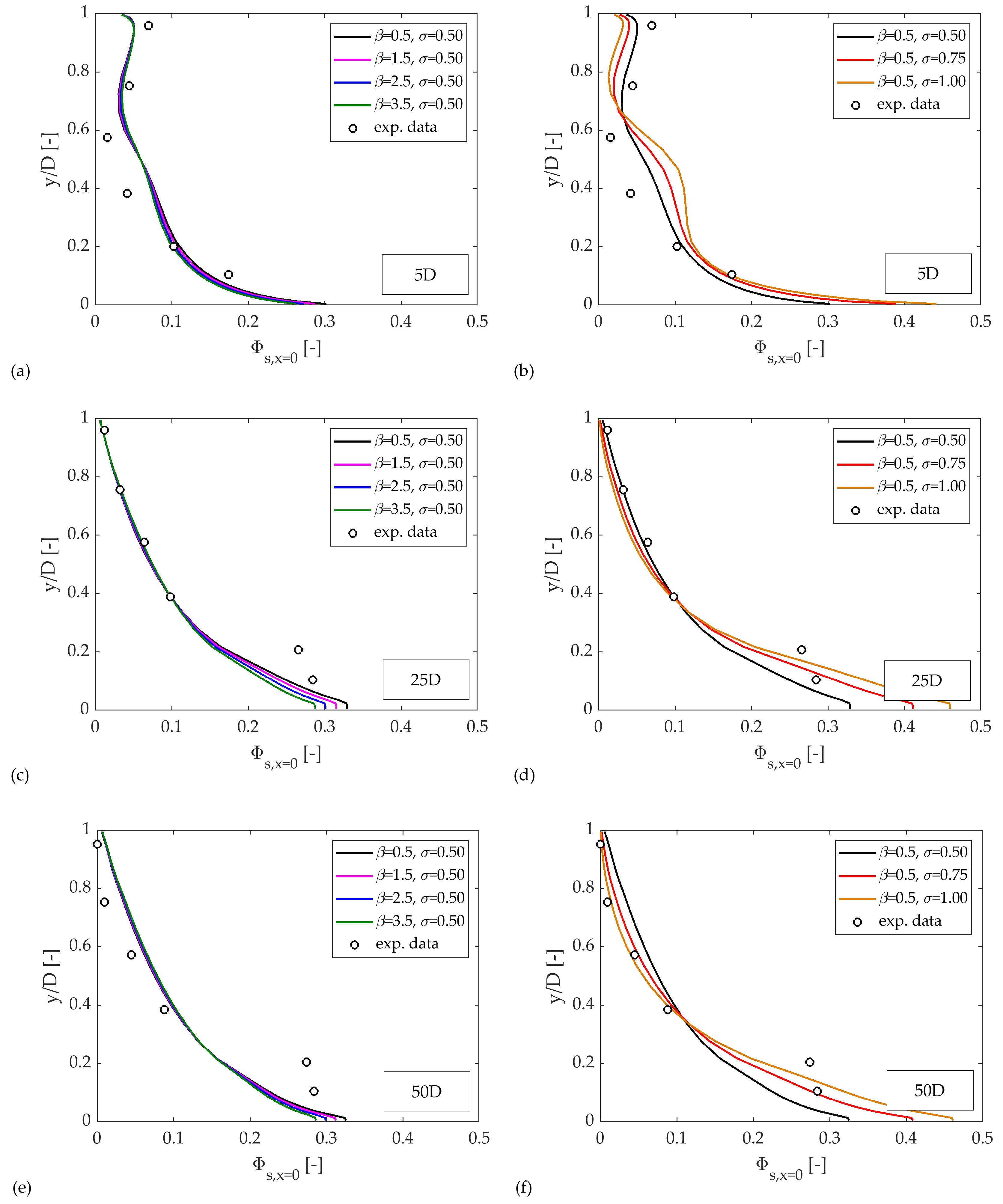
4.2.5. Effect of the Calibration Coefficients and Comparison with Experiments

As a conclusion of this test case, the predictive capacity of the betaSigmaSlurryFoam solver was investigated by making a sensitivity analysis of the solution with respect to the values of the tuning parameters $\beta$ and $\sigma$ and performing a comparison with the experimental data from Kaushal et al. [29].

Firstly, we focused on the experiment carried out in the absence of particles, with the aim of testing the suitability of some features of the betaSigmaSlurryFlow model that plays a role also in single-phase conditions, such as the turbulence model. As anticipated, we decided to use the k-$\omega$ SST turbulence model based on the findings of our previous work [40]. However, some differences exist between the experiment by Sudo et al. [44], considered in [40], and the current test by Kaushal et al. [29]. For instance, in the experiment of Sudo and co-workers, the bulk Reynolds number, Re, and the radius ratio, $R_{\mathrm{b}}/R$ were $6.2\times {10}^4$ and 4.0, respectively; in the test by Kaushal and co-workers, they were $1.89\times {10}^5$ and 5.6. Additionally, the pipe was hydraulically smooth in the set up of Sudo and co-workers, whereas a non negligible relative roughness of 0.0003 was reported in that of Kaushal and co-workers. Figure 16 compares the $C_{\mathrm{p}}^{\mathrm{w}}$ profiles along the intrados and the extrados, as obtained by OpenFOAM, and the experimental results by Kaushal et al. [29]. Note that each experimental point provided by the experimenters was the average of two pressure taps located at the intrados and at the extrados, and that all data have been have been adjusted to have $C_{\mathrm{p}}^{\mathrm{w}}$ = 0 at the intrados of the section 8D downstream of the bend. Although the numerical results agreed with the experimental data from a qualitative point of view, there are obvious differences, which deserved some investigation; particularly, the calculated bend loss coefficient $k_{\mathrm{t}}$ was 0.277, about 30% lower than the measured value of 0.392. Note that, in [40], the same single-phase fluid dynamic model yielded very good prediction of $C_{\mathrm{p}}^{\mathrm{w}}$ at both intrados and extrados for the experimental test of Sudo et al. [44], which, as just mentioned, differs from the present ones in several aspects. The considerations reported by Kaushal et al. [29] suggest that the roughness of the pipe was the main factor responsible for the deviations observed in Figure 16. Indeed, a closer look at the $C_{\mathrm{p}}^{\mathrm{w}}$ downstream of section 8D indicates that our CFD simulations tend to underestimate the frictional losses in straight pipes. Additionally, repeating the simulation assuming a hydraulically smooth pipe (that is, calling the function nutkWallFunction insead of nutkRoughWallFunction) yielded practically the same $C_{\mathrm{p}}^{\mathrm{w}}$ profiles, whereas the Moody chart indicates that, at a Reynolds number of $1.89\times {10}^5$, the friction factor in a straight pipe with relative roughness of 0.0003 is about 15% higher than the value for a hydraulically smooth pipe. This finding suggests that the combination of the k-$\omega$ SST turbulence model and the nutkRoughWallFunction might be unable to correctly capture the effect of wall roughness in the range of interest, an interpretation which is further corroborated by a report available in the literature [45]. The development of more accurate models for rough walls is needed, but this task is shelved for future research. Our objective was to assess the predictive capacity of betaSigmaSlurryFoam for a more complex case than the straight horizontal pipe one considered so far, and we believe that this goal could be achieved despite the limitations of the rough wall model. Nonetheless, the comparison against the experimental data cannot ignore the unresolved modelling issue. From this perspective, for the slurry flow cases, the validation of the bend loss coefficient was made in terms of $k_{\mathrm{t}}/k_{\mathrm{t},\mathrm{SP}}$, that is, its ratio with the single phase value, which was expected to be less sensitive to the wall roughness than the individual $k_{\mathrm{t}}$ and $k_{\mathrm{t},\mathrm{SP}}$ values.

Focusing on the three slurry flow cases, a sensitivity analysis was made for four different values of $\beta$ (0.5, 1.5, 2.5, 3.5) and three values of $\sigma$ (0.50, 0.75, 0.50). The tested combinations and the corresponding values of $k_{\mathrm{t}}/k_{\mathrm{t},\mathrm{SP}}$ are summarized in

Table 5. Effect of $\beta$ and $\sigma$ on the ratio between the pressure loss coefficient, $k_{\mathrm{t}}$ (calculated as in Equation (23)), and the corresponding single phase value, $k_{\mathrm{t},\mathrm{SP}}$: comparison between CFD predictions and experimental measurements for the three concentration levels.

		${\mathit{C}}_{\mathbf{in}}$ = 0.0394		${\mathit{C}}_{\mathbf{in}}$ = 0.0882		${\mathit{C}}_{\mathbf{in}}$ = 0.1628
$\mathit{\beta }$	$\mathit{\sigma }$	CFD	Exp.	CFD	Exp.	CFD	Exp.
0.5	0.50	0.996	0.999	1.102	1.225	1.331	1.328
1.5		1.002		1.130		1.408
2.5		1.009		1.161		1.500
3.5		1.016		1.197		1.604
0.50	0.50	0.996	0.999	1.102	1.225	1.331	1.328
	0.75	1.035		1.185		1.442
	1.00	1.073		1.251		1.524

, alongside with the experimentally measured values. For the three values of $C_{\mathrm{in}}$, increasing either of the two parameters results in higher loss coefficient. Such effect is quite small at $C_{\mathrm{in}}$ = 0.0394, but it becomes noticeable at $C_{\mathrm{in}}$ = 0.0882 and 0.1628; from a certain standpoint, this marks a difference from the previous horizontal pipe case, where the effect of these two parameters on the hydraulic gradient was sensible only at much higher concentration levels (Table 3). This finding confirms the higher fluid dynamic complexity of a bend flow compared to the flow in a straight pipe, and, specifically, highlights that different physical mechanisms come into play in determining the related energy losses. In order to achieve a more complete picture of the pressure distribution, Figure 17 shows the streamwise wall pressure profile at the intrados and at the extrados of the pipe for the three test cases and the six combinations of $\beta$ and $\sigma$. On the horizontal axes, we highlighted sections −2D (two pipe diameters upstream of the bend entrance) and 8D (eight pipe diameters downstream of the bend exit), which were those used for the calculations of $k_{\mathrm{t}}$. The $C_{\mathrm{p}}^{\mathrm{w}}$ curves were translated to have a null value at the intrados of section +8D. The observations previously made for $k_{\mathrm{t}}/k_{\mathrm{t},\mathrm{SP}}$ hold for the entire set of $C_{\mathrm{p}}^{\mathrm{w}}$ profiles. At $C_{\mathrm{in}}$ = 0.0394, the $C_{\mathrm{p}}^{\mathrm{w}}$ profiles are practically unaffected by $\beta$ and $\sigma$; at $C_{\mathrm{in}}$ = 0.0882, the effect of $\sigma$ starts to be visible; at $C_{\mathrm{in}}$ = 0.1628, the influence of both $\beta$ and $\sigma$ is obvious. A more detailed look at the plots shows that, even at the highest concentration levels, $\beta$ and $\sigma$ do not have an impact on the linear decrease of $C_{\mathrm{p}}^{\mathrm{w}}$ downstream the bend and that, at the same time, the linear $C_{\mathrm{p}}^{\mathrm{w}}$ profiles upstream of the bend are nearly parallel to each other. This suggests that, whenever an effect of $\beta$ and $\sigma$ on the pressure field is detected, this is confined to the bend region, whereas the frictional losses in the upstream and downstream pipes, quantified by the slope of the linear branches of the $C_{\mathrm{p}}^{\mathrm{w}}$ profiles, are practically insensitive to the values of the two coefficients. This finding was not surprising since, as partially demonstrated in Table 3, the effect of $\beta$ and $\sigma$ on the hydraulic gradient of straight pipe flow becomes sensitive only at concentration levels higher than those of the present bend experiments (0.0394, 0.0882, and 0.1628).

The study of the influence of $\beta$ and $\sigma$ was extended to the two parameters related with the velocity field of the liquid phase, namely, the intensity of the secondary flow, $I_{\mathrm{s},\mathrm{l}}$ (Equation (21)), and the turbulent energy parameter, $k_{\mathrm{a},\mathrm{l}}$ (Equation (22)). As shown in Figure 18 and Figure 19, the effects of the two coefficients on $I_{\mathrm{s},\mathrm{l}}$ and $k_{\mathrm{a},\mathrm{l}}$ are quite similar to those observed for the pressure-related parameters, $k_{\mathrm{t}}$ and $C_{\mathrm{p}}^{\mathrm{w}}$. Specifically, increasing either $\beta$ or $\sigma$ increases both the intensity of the secondary flow and the level of turbulence in the liquid phase. It is difficult to give a definitive interpretation for these findings, due to the complexity of the fluid dynamics model and the interplay of different features. The effect of $\sigma$ on $k_{\mathrm{a},\mathrm{l}}$ might be explained by considering that a higher $\sigma$ induces the particles to travel in the bottom part of the pipe, pushing the liquid to move in the upper part at higher velocity, hence generating high turbulence levels.

Finally, the sensitivity analysis was extended to the solid volume fraction distribution, making specific reference to the vertical profiles of ${\Phi }_{\mathrm{s}}$ at sections 5D, 25D, and 50D downstream of the bend exit. The results are shown in Figure 20, Figure 21 and Figure 22 for the three concentration levels. At 50D (plots (e) and (f)), the slurry flow has practically recovered and, not surprisingly, the effects of $\beta$ and $\sigma$ are as expected for a straight pipe case. That is, the effect of $\beta$ is practically undetectable even at the higher $C_{\mathrm{in}}$, whereas a larger $\sigma$ dampened the turbulent dispersion of the particles inducing them to occupy the lower part of the pipe. The influence of $\beta$ remains mild even in the two other sections, whereas the effect of $\sigma$ is obvious. Specifically, the enhancement of turbulent dispersion brought by a lower $\sigma$ reflects in a flatter concentration profile; conversely, a higher $\sigma$ produces higher solid concentration in the central region of the pipe section, as a result of the complex interplay between the solids and the secondary flow pattern.

As a conclusion to this study, a comparison with the experimental data from Kaushal et al. [29] was made to assess the overall level of accuracy of the betaSigmaSlurryFlow solver, taking into account the sensitivity of the solution with respect to the values of $\beta$ and $\sigma$. Specifically, the comparison was made in terms of the $k_{\mathrm{t}}/k_{\mathrm{t},\mathrm{SP}}$ ratio, that is, the ratio of the bend loss coefficient in slurry conditions to that in single-phase conditions, and the vertical concentration profiles at sections 5D and 25D. The calculated and the measured values of $k_{\mathrm{t}}/k_{\mathrm{t},\mathrm{SP}}$ as well as of the vertical concentration profiles are compared in Table 5 and in Figure 20 and Figure 21, respectively. Although there is no single combination of $\beta$ and $\sigma$ that allows a perfect match between the three experimentally measured values of $k_{\mathrm{t}}/k_{\mathrm{t},\mathrm{SP}}$, for every is ($\beta$, $\sigma$), the betaSigmaSlurryFlow solver was able to capture the increasing trend of the bend loss coefficient with solid concentration. It should also be noted that the experimental values of $k_{\mathrm{t}}$ and $k_{\mathrm{t},\mathrm{SP}}$ reported in Table 5 were obtained by extracting the $C_{\mathrm{p}}^{\mathrm{w}}$ data points from the published article, and this might have produced inaccuracies which added to the experimental error. As for the vertical concentration profiles, in this case, the experimental data points were digitized from the figures in the paper, and no uncertainty bars were provided. Nonetheless, the model appears able to capture the distortion of the solid concentration profile produced by the bend compared to the straight pipe configuration. Although the considerations above prevented the accurate comparison of experiments and simulations, the combination $\beta$ = 0.5 and $\sigma$ = 0.5 appeared the best among those considered. Importantly, these values were compatible with our previous investigations on straight pipe flows. Specifically, in [46], we found that the appropriate value for $\sigma$ increases with increasing pipe diameter, obtaining 0.5 for a pipe diameter of the order of 50 mm, which is the case for the pipe bend experiments of Kaushal et al. [29]. At the same time, in [10], we found that values of $\beta$ in the order of 0.25–0.50 were appropriate to simulate the transport of silica sand particles.

5. Conclusions

The following achievements have been reached through this research.

• We developed and shared with the scientific community betaSigmaSlurryFoam, a fully open source implementation of our earlier $\beta$-$\sigma$ two-fluid model for the simulation of fully suspended slurry transport in pipes within the OpenFOAM platform.
• We demonstrated the similarity between betaSigmaSlurryFoam, implemented in OpenFOAM, and the earlier $\beta$-$\sigma$ two-fluid model, implemented in PHOENICS, for horizontal slurry pipe transport in different testing conditions. We found not only that the two solutions are very close to each other, but also that the effects of $\beta$ and $\sigma$ are the same for the two implementations, confirming that the same calibration procedures could be used.
• We successfully assessed the predictive capacity of betaSigmaSlurryFoam for the more complex case of slurry transport in a horizontal pipe bend, which was not considered in our previous works of the $\beta$-$\sigma$ two-fluid model, referring to some experimental tests carried out by Kaushal et al. [29]. Two features in particular made the results fully satisfactory. Firstly, betaSigmaSlurryFoam showed physical consistency and good agreement with the experimental data also for slightly coarser particles than those considered so far. Secondly, the suitable combination of $\beta$ and $\sigma$ in the case of pipe bend flow was in line with the values obtained in previous studies on straight horizontal pipes with similar diameter and type of particles.

Hence, the betaSigmaSlurryFlow solver has proven an engineering-effective tool which, with a simple mathematical structure and only two main calibration coefficients, was capable of predicting the most relevant features of slurry transport not only in straight pipes, but also in pipe bends. In terms of the future scope of this research, we mention the application of betaSigmaSlurryFlow to deepen insight into the behavior of slurry transport in straight pipes and bends at varying conditions, e.g., velocity, concentration, particle type, pipe diameter, pipe roughness etc., as well its use to obtain useful information for the design and the management of complex devices of interest in slurry technology, such as pumps or valves. At the same time, we aim at fostering the collaboration of researchers in the field of CFD slurry flow modelling to achieve the long-term goal of developing a unified model for slurry transport over different regimes, which would be include, within the same framework, the effects of particle–turbulence interactions, particle–particle collisions, and particle–particle contacts.

References

1. Visintainer, R.; Matoušek, V.; Pullum, L.; Sellgren, A. Slurry Transport Using Centrifugal Pumps; Springer: Berlin/Heidelberg, Germany, 2023. [Google Scholar]
2. Lareo, C.; Fryer, P.J.; Barigou, M. The fluid mechanics of two-phase solid-liquid food flows: A review. Food Bioprod. Process. 1997, 75, 73–105. [Google Scholar] [CrossRef]
3. Jiang, Y.Y.; Zhang, P. Numerical investigation of slush nitrogen flow in a horizontal pipe. AIChE J. 2012, 59, 1762–1773. [Google Scholar] [CrossRef]
4. Alvarado, J.L.; Marsh, C.; Sohn, C.; Phetteplace, G.; Newell, T. Thermal performance of microencapsulated phase change material slurry in turbulent flow under constant heat flux. Int. J. Heat Mass Transf. 2007, 50, 1938–1952. [Google Scholar] [CrossRef]
5. Singh, M.K.; Kumar, S.; Ratha, D.; Kaur, H. Design of slurry transportation pipeline for the flow of muti-particulate coal ash suspension. Int. J. Hydrogen Energy 2017, 42, 19135–19138. [Google Scholar] [CrossRef]
6. Quarini, G.; Aislie, E.; Ash, D.; Leiper, A.; McBryde, D.; Hebert, M.; Deans, T. Transient thermal performance of ice slurries pumped through pipes. Appl. Therm. Eng. 2021, 50, 743–748. [Google Scholar] [CrossRef]
7. Messa, G.V.; Yang, Q.; Adedeji, O.E.; Chára, Z.; Duarte, C.A.R.; Matoušek, V.; Rasteiro, M.G.; Sanders, R.S.; Silva, R.C.; de Souza, F.J. Computational Fluid Dynamics Modelling of Liquid-Solid Slurry flows in Pipelines: State-of-the-Art and Future Perspectives. Processes 2021, 9, 1566. [Google Scholar] [CrossRef]
8. Messa, G.V.; Matoušek, V. Analysis and discussion of two-fluid modelling of pipe flow of fully suspended slurry. Powder Technol. 2020, 360, 747–768. [Google Scholar] [CrossRef]
9. Messa, G.V.; Malin, M.; Matoušek, V. Parametric study of the β-σ two-fluid model for simulating fully suspended slurry flow: Effect of flow conditions. Meccanica 2021, 56, 1047–1077. [Google Scholar] [CrossRef]
10. Messa, G.V.; Yang, Q.; Rasteiro, M.G.; Faia, P.; Matoušek, V.; Silva, R.; Garcia, F. Computational fluid dynamic modelling of fully-suspended slurry flows in horizontal pipes with different solids concentrations. KONA Powder Part. J. 2023, 40, 219–235. [Google Scholar] [CrossRef]
11. Ekambara, K.; Sanders, R.; Nandakumar, K.; Masliyah, J. Hydrodynamic Simulation of Horizontal Slurry Pipeline Flow Using ANSYS-CFX. Ind. Eng. Chem. Res. 2009, 48, 8159–8171. [Google Scholar] [CrossRef]
12. Gopaliya, M.K.; Kaushal, D.R. Analysis of effect of grain size on various parameters of slurry flow through pipeline using CFD. Particul. Sci. Technol. 2015, 33, 369–384. [Google Scholar] [CrossRef]
13. Gopaliya, M.K.; Kaushal, D.R. Modeling of sand-water slurry flow through horizontal pipe using CFD. J. Hydrol. Hydromech. 2016, 64, 261–272. [Google Scholar] [CrossRef]
14. Kaushal, D.R.; Thinglas, T.; Tomita, Y.; Kuchii, S.; Tsukamoto, H. CFD modeling for pipeline flow of fine particles at high concentration. Int. J. Multiphase Flow 2012, 43, 85–100. [Google Scholar] [CrossRef]
15. Singh, M.K.; Kumar, S.; Ratha, D. Computational analysis on disposal of coal slurry at high solid concentrations through slurry pipeline. Int. J. Coal Prep. Util. 2020, 40, 116–130. [Google Scholar] [CrossRef]
16. Kumar, N.; Gopaliya, M.K.; Kaushal, D.R. Experimental investigations and CFD modeling for flow of highly concentrated iron ore slurry through horizontal pipeline. Part. Sci. Technol. 2018, 37, 232–250. [Google Scholar] [CrossRef]
17. Krampa, F.N. Two-Fluid Modelling of Heterogeneous Coarse Particle Slurry Flows. Ph.D. Thesis, University of Saskatchewan, Saskatoon, Saskatchewan, 2009. [Google Scholar]
18. Antaya, C.L.; Adane, K.F.K.; Sanders, R.S. Modelling concentrated slurry pipeline flows. In Proceedings of the ASME 2012 Fluids Engineering Summer Meeting, Rio Grande, Puerto Rico, 8–12 July 2012. [Google Scholar]
19. Ofei, T.N.; Ismail, A.Y. Eulerian-Eulerian simulation of particle-liquid slurry flow in horizontal pipe. J. Pet. Eng. 2016, 37, 232–250. [Google Scholar] [CrossRef]
20. Lapworth, L. Hydra-CFD: A framework for collaborative CFD development. In Proceedings of the International Conference on Scientific and Engineering Computation, Singapore, 30 June–2 July 2004. [Google Scholar]
21. Fiorina, C.; Shriwise, P.; Dufresne, A.; Ragusa, J.; Ivanov, K.; Valentine, T.; Lindley, B.; Kelm, S.; Shwageraus, E.; Monti, S.; et al. An initiative for the development and application of open-source multi-physics simulation in support of R&D and E&T in nuclear science and technology. In Proceedings of the PHYSOR2020—International Conference on Physics of Reactors: Transition to a Scalable Nuclear Future, Cambridge, UK, 30 March–2 April 2020. [Google Scholar]
22. Kodman, J.B.; Singh, B.; Murugaiah, M. A Comprehensive Survey of Open-Source Tools for Computational Fluid Dynamics Analyses. J. Adv. Res. Fluid Mech. Therm. Sci. 2024, 119, 123–148. [Google Scholar] [CrossRef]
23. Shouten, T.D.; Keetels, G.H.; van Rhee, C. Suspended pipeflow with OpenFOAM. In Proceedings of the 19th International Conference on Transport and Sedimentation of Solid Particles, Cape Town, South Africa, 24–27 September 2019. [Google Scholar]
24. Shouten, T.D.; van Rhee, C.; Keetels, G.H. Two-phase modelling for sediment water mixtures above the limit deposit velocity in horizontal pipelines. J. Hydrol. Hydromech. 2021, 3, 263–274. [Google Scholar] [CrossRef]
25. Reyes, C.; Ihle, C.F. Numerical simulation of cation exchange in fine-coarse seawater slurry pipeline flow. Miner. Eng. 2018, 117, 14–23. [Google Scholar] [CrossRef]
26. Mackenzie, A.; Stickland, M.T.; Dempster, W.M. Development of a Combined Euler-Euler Euler-Lagrange Slurry Model. In OpenFOAM: Selected Papers of the 11th Workshop; Nóbrega, J.M., Jasak, H., Eds.; Springer: Cham, Switzerland, 2019; pp. 77–92. [Google Scholar]
27. Liu, X.; Yuan, A.; Li, Y.; Wang, Z.; Wang, Z.; Liu, Z.; Wang, W. Numerical simulation of hydrate slurry flow and deposit behavior based on openfoam-IATE. Fuel 2022, 310, 122426. [Google Scholar] [CrossRef]
28. Ghoudi, Z.; Benckhaldoun, F.; Piscaglia, F.; Hajjaji, N. Towards the modeling of the effect of turbulent water batches on the flow of slurries in horizontal pipes using CFD. Eur. J. Mech. B Fluids 2023, 100, 208–222. [Google Scholar] [CrossRef]
29. Kaushal, D.R.; Kumar, A.; Tomita, Y.; Kuchii, S.; Tsukamoto, H. Flow of mono-dispersed particles through horizontal bend. Int. J. Multiphase Flow 2013, 52, 71–91. [Google Scholar] [CrossRef]
30. Spalding, D.B. Numerical computation of multi-phase fluid flow and heat transfer. In Recent Advances in Numerical Methods in Fluids; Taylor, C., Morgan, K., Eds.; Pineridge Press Limited: Swansea, UK, 1980; Volume 1, pp. 139–168. [Google Scholar]
31. The PHOENICS Encyclopedia: Two-Phase Flows. Available online: https://www.cham.co.uk/phoenics/d_polis/d_lecs/ipsa/ipsa.htm (accessed on 6 December 2024).
32. Launder, B.E.; Spalding, D.B. The numerical computation of turbulent flows. Comput. Meth. Appl. Mech. Eng. 1974, 3, 269–289. [Google Scholar] [CrossRef]
33. Models for Two-Phase Flow: Two-Equation k-ε Turbulence Model. Available online: https://www.cham.co.uk/phoenics/d_polis/d_enc/turmod/enc_tu74.htm (accessed on 6 December 2024).
34. Schiller, L.; Naumann, A. A drag coefficient correlation. Z. Ver. Deutsch. Ing. 1935, 77, 318–320. [Google Scholar]
35. Cheng, N.S.; Law, A.W.K. Exponential formula for computing effective viscosity. Powder Technol. 2003, 129, 156–160. [Google Scholar] [CrossRef]
36. The PHOENICS Encyclopedia: Equilibrium Log-Law Wall Functions. Available online: https://www.cham.co.uk/phoenics/d_polis/d_enc/turmod/enc_tu82.htm (accessed on 6 December 2024).
37. Massey, B.S.; Ward-Smith, J. Mechanics of Fluids; Taylor & Francis: London, UK, 2006. [Google Scholar]
38. Thomas, A. A modification of the Wilson & Judge deposit velocity equation, extending its applicability to finer particles and larger pipe sizes. In Proceedings of the 17th International Conference of Transport and Sedimentation of Solid Particles, Delft, The Netherlands, 22–25 September 2015. [Google Scholar]
39. Korving, A.C. High concentrated fine-sand slurry flow in pipelines: Experimental study. In Proceedings of the 15th International Conference on Hydrotransport, Banff, AB, Canada, 3–5 June 2002. [Google Scholar]
40. Yang, Q.; Dong, J.; Xing, T.; Zhang, Y.; Guan, Y.; Liu, X.; Tian, Y.; Peng, Y. RANS-Based Modelling of Turbulent Flow in Submarine Pipe Bends: Effect of Computational Mesh and Turbulence Modelling. J. Mar. Sci. Eng. 2023, 11, 336. [Google Scholar] [CrossRef]
41. Passalacqua, A.; Fox, R.O. Implementation of an iterative solution procedure for multi-fluid gas–particle flow models on unstructured grids. Powder Technol. 2011, 213, 174–187. [Google Scholar] [CrossRef]
42. Sweby, P.K. High resolution schemes using flux limiters for hyperbolic conservation laws. SIAM J. Numer. Anal. 1984, 21, 995–1011. [Google Scholar] [CrossRef]
43. Gillies, R.G. Pipeline Flow of Coarse Particle Slurries. Ph.D. Thesis, University of Saskatchewan, Saskatoon, Saskatchewan, 1993. [Google Scholar]
44. Sudo, K.; Sumida, H.; Hibara, H. Experimental investigation on turbulent flow in a circular-sectioned 90-degree bend. Exp. Fluids 1998, 25, 42–49. [Google Scholar] [CrossRef]
45. Thomas, T. Friction Factor in Internal Pipe Turbulent Flow; Internship Report; Indian Institute of Technology: Bombay, India, 2022. [Google Scholar]
46. Yang, Q.; Messa, G.V.; Matoušek, V. Towards the assessment of the predictive capacity of the β-σ two-fluid model for pseudo-homogeneous slurry flow in pipes. In Proceedings of the 20th International Conference on Transport and Sedimentation of Solid Particles, Wroclaw, Poland, 26–29 September 2023. [Google Scholar]
Figure 1. Effect of coefficient β on the relation between the friction parameter, μ ˜ m , and the local solid volume fraction, Φ s .
Processes 12 02863 g001
Figure 2. Flow chart of the betaSigmaSlurryFoam solver.
Processes 12 02863 g002
Figure 3. Horizontal pipe case: (a) computational domain and boundary conditions; (b) layouts of the four computational meshes over the pipe section used for the grid independence study. Mesh 3 was employed for the subsequent similarity assessment analysis.
Processes 12 02863 g003
Figure 4. Exemplary results for case C1: (a) time histories of the chord-average solid concentration, Φ s γ , and of the eddy viscosity of the liquid, at the center of the pipe outlet, normalized by the values at t = 10 s; (b) axial development of the same variables at t = 5 s, normalized by the values at the pipe outlet, at two locations along the vertical pipe diameter.
Processes 12 02863 g004
Figure 5. Vertical profiles of (a) the chord-average solid concentration, Φ s γ , and of (b) the eddy viscosity of the liquid, ν l t , calculated on the four O-type meshes in Figure 3 for case C1.
Processes 12 02863 g005
Figure 6. Effect of the thickness of the near wall cells, in terms of y + , on the predicted hydraulic gradient, i m , for cases C1 and C6: comparison of betaSigmaSlurryFoam in OpenFOAM and the β - σ two-fluid model in PHOENICS.
Processes 12 02863 g006
Figure 7. Sensitivity analysis on the chord averaged solid volume fraction profile: (a) effect of varying β for case C1, with σ = 0.75; (b) effect of varying σ for case C1, with β = 2.5; (c) effect of varying β for case C6, with σ = 0.75; (d) effect of varying σ for case C6, with β = 2.5 (continuous lines: predictions of betaSigmaSlurryFoam using OpenFOAM; dotted lines: predictions of β - σ two-fluid model using PHOENICS).
Processes 12 02863 g007
Figure 8. Horizontal pipe bend case: (a) computational and boundary conditions; (b) detail of the “mesh 3” discretization in the bend region.
Processes 12 02863 g008
Figure 9. Case C in = 0.0882 with β = 0.5 and σ = 0.5: wall pressure coefficient along the streamwise coordinate at the intrados ( θ = 0°) and the extrados ( θ = 180°) of the pipe bend.
Processes 12 02863 g009
Figure 10. Case V m = 3.56 m/s and C in = 0.0882 with β = 0.5 and σ = 0.5: contours of the normalized streamwise velocity of the liquid at different sections inside of the bend and downstream of it. The left and right sides of each figure show the extrados and the intrados of the bend, respectively.
Processes 12 02863 g010
Figure 11. Case C in = 0.0882 with β = 0.5 and σ = 0.5: pattern of the secondary velocity vectors of the liquid at different sections inside of the bend and downstream of it. The left and right sides of each figure show the extrados and the intrados of the bend, respectively.
Processes 12 02863 g011
Figure 12. Case C in = 0.0882 with β = 0.5 and σ = 0.5: streamwise profiles of (a) secondary flow intensity of the liquid phase and (b) turbulent energy parameters of the liquid phase.
Processes 12 02863 g012
Figure 13. Case V m = 3.56 m/s and C in = 0.0882 with β = 0.5 and σ = 0.5: contours of the magnitude of the relative velocity at different sections inside of the bend and downstream of it. The left and right sides of each figure show the extrados and the intrados of the bend, respectively.
Processes 12 02863 g013
Figure 14. Case V m = 3.56 m/s and C in = 0.0882 with β = 0.5 and σ = 0.5: contours of the solid volume fraction at different sections inside of the bend and downstream of it. The left and right sides of each figure show the extrados and the intrados of the bend, respectively.
Processes 12 02863 g014
Figure 15. Case C in = 0.0882 with β = 0.5 and σ = 0.5: effect of the mesh on the streamwise profiles of (a) C p w (at intrados and extrados), of (b) I s , l , and of (c) k a , l , and (d) on the solid volume fraction profile along the vertical diameter of section 5D downstream the bend exit.
Processes 12 02863 g015
Figure 16. Single-phase case: wall pressure coefficient along the streamwise coordinate at the intrados and the extrados of the pipe bend and experimental data by Kaushal et al. [29]. The experimental points colored in red are those used for the calculation of the bend loss coefficient.
Processes 12 02863 g016
Figure 17. Sensitivity analysis on the wall pressure coefficient along the streamwise coordinate at the intrados (continuous lines) and at the extrados (dotted lines) of the pipe bend: (a) effect of varying β for C in = 0.0394, with σ = 0.5; (b) effect of varying σ for C in = 0.0394, with β = 0.5; (c) effect of varying β for C in = 0.0882, with σ = 0.5; (d) effect of varying σ for C in = 0.0882, with β = 0.5; (e) effect of varying β for C in = 0.1628, with σ = 0.5; (f) effect of varying σ for C in = 0.1628, with β = 0.5.
Processes 12 02863 g017
Figure 18. Sensitivity analysis on the streamwise profile of the secondary flow intensity of the liquid phase: (a) effect of varying β for C in = 0.0394, with σ = 0.5; (b) effect of varying σ for C in = 0.0394, with β = 0.5; (c) effect of varying β for C in = 0.0882, with σ = 0.5; (d) effect of varying σ for C in = 0.0882, with β = 0.5; (e) effect of varying β for C in = 0.1628, with σ = 0.5; (f) effect of varying σ for C in = 0.1628, with β = 0.5.
Processes 12 02863 g018
Figure 19. Sensitivity analysis on the streamwise profile of the turbulent energy parameter of the liquid phase: (a) effect of varying β for C in = 0.0394, with σ = 0.5; (b) effect of varying σ for C in = 0.0394, with β = 0.5; (c) effect of varying β for C in = 0.0882, with σ = 0.5; (d) effect of varying σ for C in = 0.0882, with β = 0.5; (e) effect of varying β for C in = 0.1628, with σ = 0.5; (f) effect of varying σ for C in = 0.1628, with β = 0.5.
Processes 12 02863 g019
Figure 20. Sensitivity analysis on the solid concentration profile along the vertical diameter for C in = 0.0394: (a) section 5D downstream the bend exit, effect of varying β with σ = 0.5; (b) section 5D downstream the bend exit, effect of varying σ with β = 0.5; (c) section 25D downstream the bend exit, effect of varying β with σ = 0.5; (d) section 25D downstream the bend exit, effect of varying σ with β = 0.5; (e) section 50D downstream the bend exit, effect of varying β with σ = 0.5; (f) section 50D downstream the bend exit, effect of varying σ with β = 0.5.
Processes 12 02863 g020
Figure 21. Sensitivity analysis on the solid concentration profile along the vertical diameter for C in = 0.0882: (a) section 5D downstream the bend exit, effect of varying β with σ = 0.5; (b) section 5D downstream the bend exit, effect of varying σ with β = 0.5; (c) section 25D downstream the bend exit, effect of varying β with σ = 0.5; (d) section 25D downstream the bend exit, effect of varying σ with β = 0.5; (e) section 50D downstream the bend exit, effect of varying β with σ = 0.5; (f) section 50D downstream the bend exit, effect of varying σ with β = 0.5.
Processes 12 02863 g021
Figure 22. Sensitivity analysis on the solid concentration profile along the vertical diameter for C in = 0.1628: (a) section 5D downstream the bend exit, effect of varying β with σ = 0.5; (b) section 5D downstream the bend exit, effect of varying σ with β = 0.5; (c) section 25D downstream the bend exit, effect of varying β with σ = 0.5; (d) section 25D downstream the bend exit, effect of varying σ with β = 0.5; (e) section 50D downstream the bend exit, effect of varying β with σ = 0.5; (f) section 50D downstream the bend exit, effect of varying σ with β = 0.5.
Processes 12 02863 g022