1. Introduction
Rare Earth Elements (REEs), also known as industrial vitamins [
1], have been widely used in various fields such as metallurgy, high-speed trains, and the national defense military industry [
2]. The cascade extraction process, which is a cascade of many extraction tanks, is widely used to improve the purity of REs [
3]. As a typical complex industrial process, the Rare Earth Extraction Process (REEP) is usually characterized by large nonlinear delays and strong coupling of various process variables [
4]. However, adjusting the controlled parameters of the REEP often relies on manual experience, which can easily leads to poor performance and instability. Workers need to spend a great deal of time adjusting the parameters to stabilize the production status of the REE, especially when the feed conditions of production change; therefore, it is necessary to simulate the REEP in advance according to process data, as process simulation can quickly and accurately grasp the changes of component content (i.e., production index) to provide a decision basis for production [
5]. At present, how to achieve process simulation for the REEP is an open problem.
Several scholars have used the extraction mechanism model to describe the REEP. In [
6], an average fraction method based on the effective separation coefficient was proposed to calculate the component content of the REEP. In [
7], a relative separation coefficient-based static calculation model was proposed to calculate the component content. Recently, Yun et al. [
8] simplified the thermodynamic equilibrium equation to calculate the equilibrium concentration of REs in different extraction tanks. However, the extraction mechanism is unclear due to the complicated physicochemical reactions of REEP, which results in a mechanistic model with poor accuracy.
With the vigorous development of artificial intelligence and deep learning [
9,
10], scholars have begun to use data-driven methods to model the REEP. Giles et al. [
11] used an artificial neural network to simulate the material transmission process for the REEP. The results showed their proposed method to be more accurate than the mechanism model. Backpropagation neural networks have also been applied to simulate the extraction equilibrium of RE solvents in order to predict the distribution ratio of rare earth elements between the organic phase and the aqueous phase [
12]. In [
13], Multiple Linear Regression (MLR), Stepwise Regression (SWR), and Artificial Neural Networks (ANNs) were used to simulate the REEP, fnding that the simulation results of the models were consistent with the actual values.
Nevertheless, it is well known that the performance of the neural networks depends on the completeness of labeled data [
14], which need to be collected from the factory at substantial time and cost. To address insufficient label data, Zheng et al. [
15] used a convolution stacked auto-encoder and t-distributed Stochastic Neighbor Embedding (t-SNE) algorithm to extract useful features from unlabeled data. In [
16], a semi-supervised training strategy with auto-encoder was proposed to automatically adjust the training process according to whether or not the input data are labeled, which makes the model learn the hidden information of the unlabeled data. Further, in [
17], a Semi-Supervised Deep Sparse Auto-Encoder (SSDSAE) with both local and nonlocal information was proposed to increase the robustness of the network for intelligent fault diagnosis of rotating machinery. From the above, it can be concluded that auto-encoder networks represent an effective solution for cases of insufficient labeled industrial data.
In addition, existing methods have only designed simple shallow models to obtain the component content of the extraction tank. However, in process simulation of the REEP it is necessary to obtain the component content of every extraction tank [
18]. Due to the limitation of having only a single hidden layer structure, shallow neural networks cannot meet this accuracy requirement, as such methods cannot accurately describe a REEP with many extraction tanks. For example, solutions based on LS-SVM [
19] or Neural Networks (NNs) [
12] are only able to display the prediction results in the final output layer. Thus, shallow models do not consider the extraction tank in the posterior sequence of REEP, the deep models can easily lead to NNs overfitting the component content of the more forward extraction tanks. Hence, it is necessary to set up many NNs with different hidden layers to obtain the component content of all extraction tanks. However, these independent neural networks cannot consider the cascade relationship between extraction tanks and computing resources. In order to solve these problems, in the current paper we innovatively propose a Multi-Branch Deep Neural Network (MBDNN). In this neural network architecture, side branches are added to the main branch, allowing the component content of the forward extraction tanks to be output earlier than in the original baseline neural network. In this way, the network outputs the component content of the cascade extraction tanks through the branch layer, which meets the process simulation requirements for the REEP.
At present, the research on MBDNNs has mainly focused on classification problems. In [
20], BranchyNet added side (lateral) branch classifiers to the traditional CNN structure, allowing image prediction results with different confidence to be output from different branches to reduce computational redundancy. Multi-Branch Neural Network (MB-Net) [
21] was proposed to solve manual annotation of different remote sensing image datasets. This approach successfully boosted the average accuracy over all transfer scenarios to 89.05%, representing an improvement over standard architectures. In [
22], Chen et al. designed an end-to-end trainable two-branch Partition and Reunion Network (PRN) for the vehicle re-identification task. Through structural innovations, multi-branch networks have achieved good results in image classification and fault diagnosis [
23,
24,
25]. However, to the best of our knowledge, this kind of MBDNN has rarely been discussed for multiple-output regression problems [
26] in complex industrial processes.
In this paper, we propose the Multi-Branch Deep Feature Fusion Network with Sparse Auto-Encoder for REEP modeling, which we call SAE-MBDFFN. We first design a multi-branch deep neural network with multiple outlets to obtain the multi-stage component content of the REEP. For SAE-MBDFFN, a multiscale feature fusion mechanism is introduced to overcome gradient disappearance. Due to the limited amount of labeled data and large amount of unlabeled data in the REEP, an unsupervised pretraining method based on stacked sparse auto-encoder is proposed to determine initial value of the hidden layer. Compared with random initialization of the parameters, the proposed unsupervised pretraining method leads to faster objective function convergence. In summary, the specific innovations of this paper are as follows:
- (1)
We propose a Multi-Branch Deep Feature Fusion Network (MBDFFN) to build a simulation model for the cascaded REEP. To overcome gradient disappearance, we introduce multiscale feature fusion in the branch layer via the residual attention structure and the branch feature short connection.
- (2)
Second, we present a stacked SAE-based unsupervised pretraining method for MBDFFN to determine the initial parameters of the network. Supervised fine-tuning on SAE-MBDFFN is then utilized to obtain the simulation model of the REEP.
- (3)
Finally, simulation results show that our proposed SAE-MBDFFN achieves better performance compared to conventional neural networks and models that do not utilize pretraining.
In summary, this paper proposes a method for simulating the Rare Earth Extraction Process (REEP) by combining prior information extraction and a multi-branch neural network. Simulation results show that the proposed method has a small error for component content prediction and is able to meet actual production needs, which can provide intelligent decision support for process reorganization and parameter optimization.
The rest of this article is structured as follows: in
Section 2, the principles of REEP and sparse auto-encoder algorithms are briefly introduced; then, the proposed multi-branch deep feature fusion network combined with SAE is described in detail in
Section 3, which also introduces the unsupervised fine-tuning training process and REEP modeling steps; subsequently, the proposed method is verified using an the RE extraction factory dataset in
Section 4; finally,
Section 5 summarizes the main contributions of this article.
2. Introduction to the Rare Earth Extraction Process (REEP) and Sparse Auto Encoders
2.1. Description of the REEP
Because the separation factor between rare earth elements (REEs) is small, it is difficult to obtain the ideal component content of REEs using only a single extraction tank. Therefore, factories usually cascade a certain number of extraction tanks to ensure that REE liquids are continuously mixed, stirred, separated, and clarified under the action of the detergent and extractant [
18].
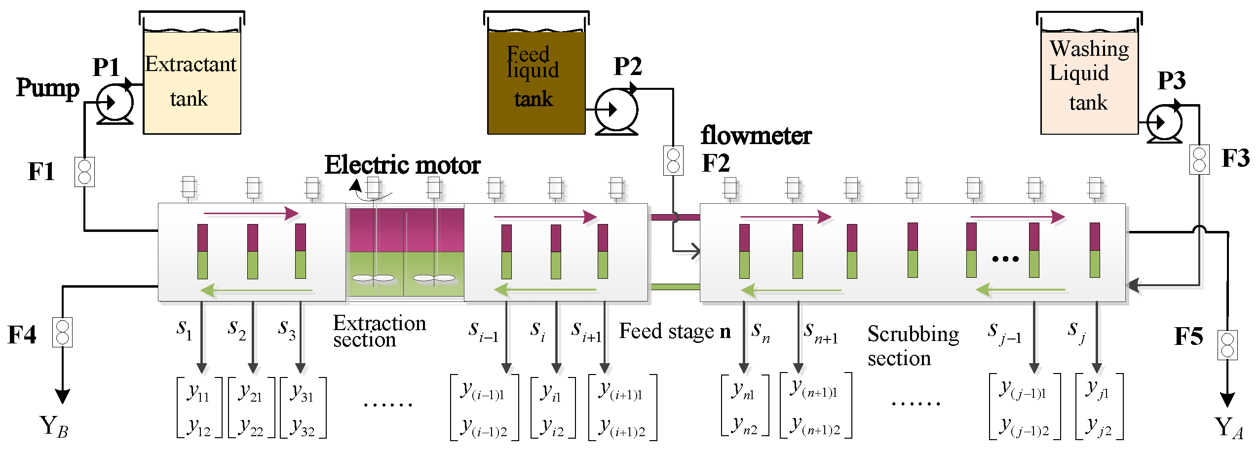
Figure 1 depicts the production flow of the REEP, which involves the stages of extraction and scrubbing. Here, j = n + m, where each stage contains the corresponding mixer–settler number.
In REEP, the detergent and extractant are injected in the first and last stages respectively, with the liquid raw material is added between these stages. Then, the rare earth liquid appears with up-and-down stratification during the clarification process. Generally, the elements in the upper solution are called easy-to-extract components (i.e., organic phase), while the elements in the lower solution are called difficult-to-extract components (i.e., aqueous phase). The upper organic-phase liquid flows from left to right, while the lower aqueous phase solution has the opposite direction. After this process, the aqueous phase product with content can be obtained from the first extraction tank, while the organic phase product with content can be obtained at the last stage. For the i-th extraction tank, the corresponding component content value is , where indicates the component content of the organic phase elements and indicates component content of the aqueous phase elements.
Obviously, when the raw rare earth solution changes, the product quality (component content) changes during the REEP as well; therefore, obtaining these changes in a timely and accurate fashion is an important prerequisite for quickly adjusting the controlled parameters during production. Process simulation of the REEP is considered to be an effective method, as it can avoid the need for workers to spend time and cost on stabilizing the production status of the REEP when the raw REE solution changes.
In the REEP, the a relationship between the component content and the feed parameters is , where represent the component contents of the stage organic and aqueous phases, respectively, represents the feed parameters, T represents external disturbances such as temperature that affect the production process, and represents a complex nonlinear function connecting the feed parameters and the component content. The goal of this paper is to develop an effective simulation model for the function .
2.2. Sparse Auto-Encoders
As shown in
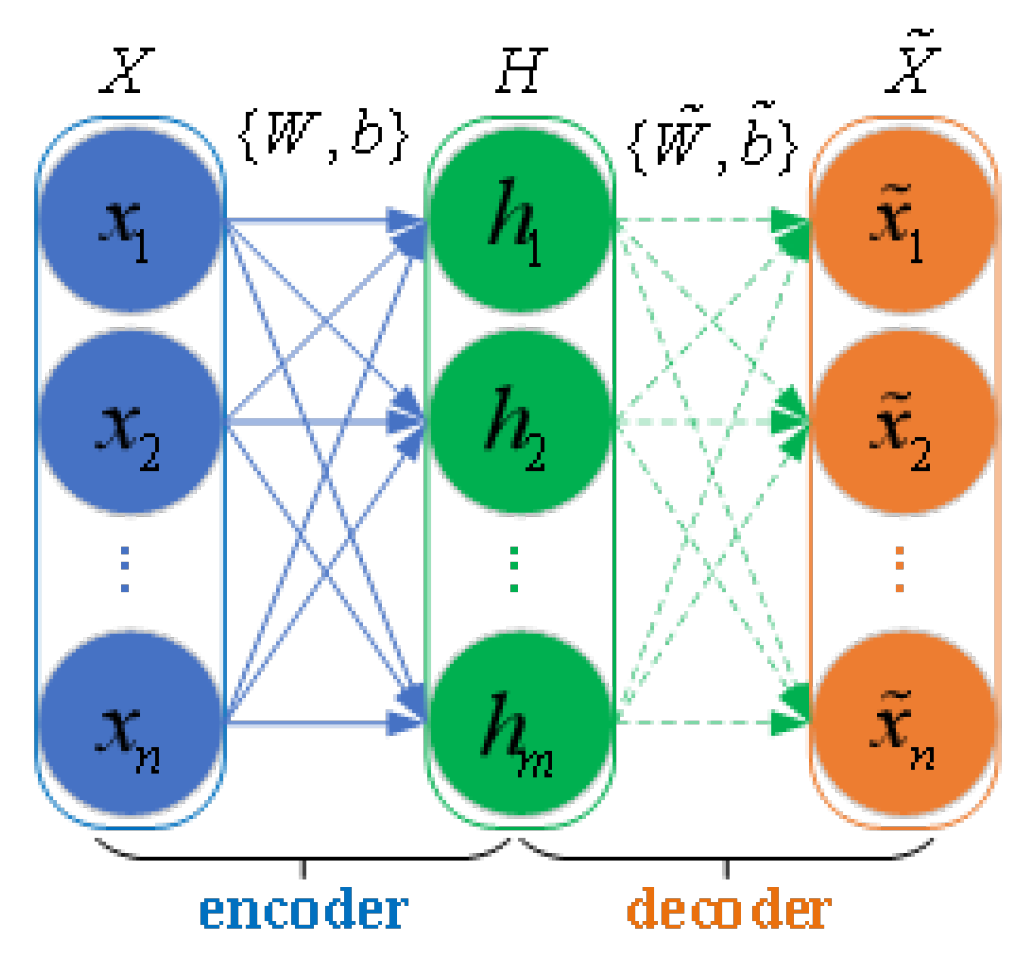
Figure 2, an Auto-Encoder (AE) [
27] is a three-layer neural network which consist of an input layer, a hidden layer, and an output layer. The encoder consists of the input layer and hidden layer, while the decoder includes the hidden layer and output layer. First, the input data are mapped as hidden features in the encoder. Then, the decoder maps the hidden feature to reconstruct the input data at the output layer. The encoder can be represented by
where
denotes n-dimensional input data,
is the hidden information, w and b respectively indicate the weight matrix and bias vector connecting the input layer and hidden layer, and
f is the activation function. Similarly, the decoder is expressed as
where
is the reconstructed output vector, while
, and
are the weight matrix, bias vector, and activation function at the output layer, respectively. To train the model parameters and obtain the feature data, the AE is trained using the reconstruction loss function of a mean squared error term, which is
.
In order to further extract key feature information and reduce feature redundancy, the Sparse Auto-Encoder (SAE) proposed in [
28] adds a sparse penalty term to the loss function, as follows:
where is the number of cells in the hidden layer,
is the constant factor of the sparse term,
is called the sparse constant, and
is the average activation amount of the
cell in the hidden layer, i.e.,
, where
represents the activation amount of the
cell in the hidden layer and
is the Kullback–Leibler (KL) divergence. The first term is the Mean Squared Error (MSE) function, while the second term is called the sparse penalty term, which calculates KL divergence value between
and
. Specifically, the KL value mathematical expression is provided as follows:
To make most neurons ‘inactive’, the SAE adds a sparse penalty term to let in a small range during the training process, ensuring that the features of the hidden layer are sparsely distributed.
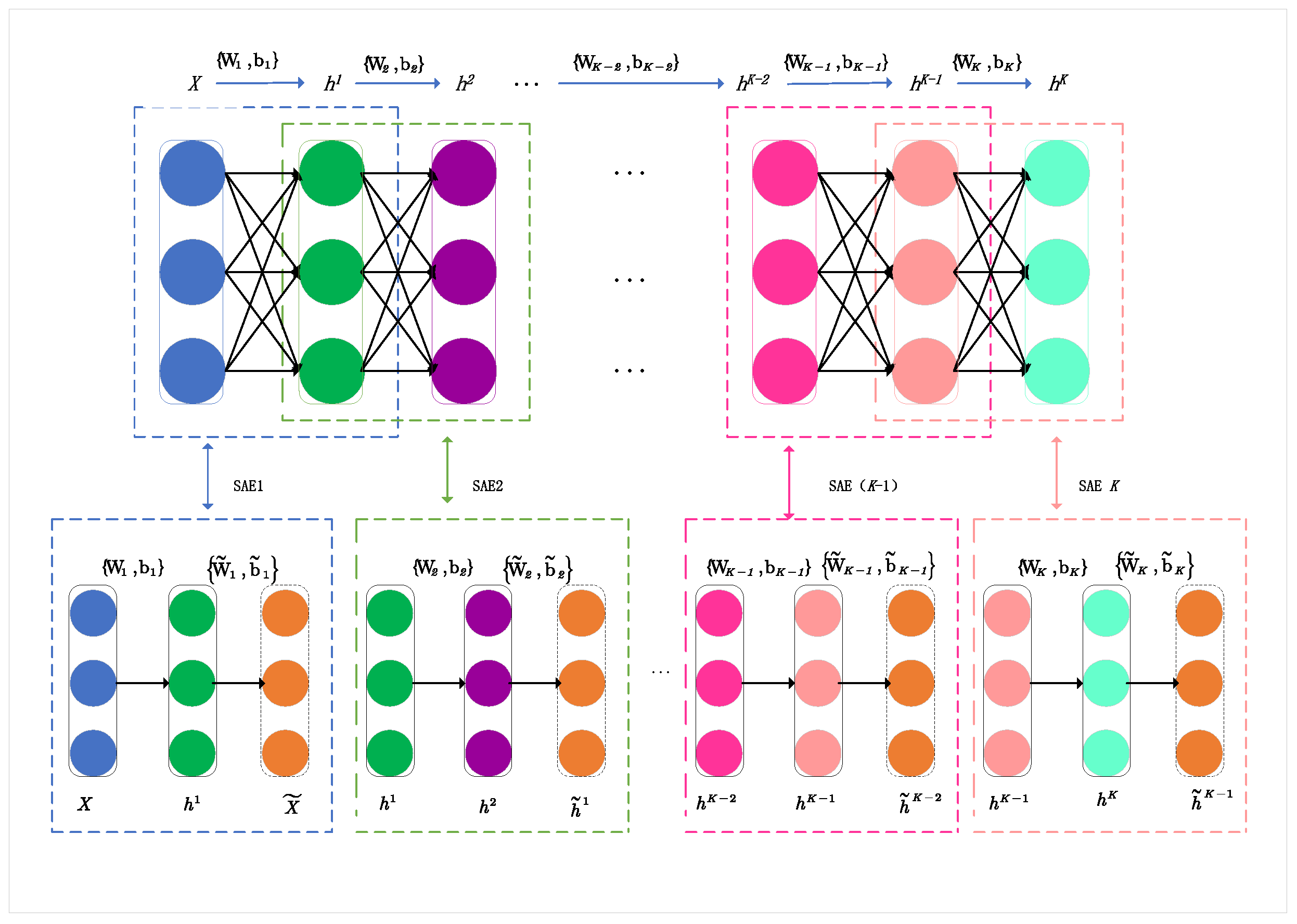
Multiple SAEs can be hierarchically stacked to form a Stacked Sparse Auto-Encoder Network (SSAE). The schematic of an SSAE is illustrated in
Figure 3. A deep SSAE network with k layers can be obtained by connecting the encoder part of each SAEs hierarchically, then continuously reconstructing the outputs of the front hidden layers. It should be noted that the decoder part of each SAE is discarded. First, the raw input data
and reconstructed data
are utilized to learn the first-layer hidden information
. Then, the remaining layers of information (h2, h3, …, hK) can be progressively calculated based on layer-wise learning. In SAE1, the encoder maps X to
with parameter set
and the decoder reconstructs the input data as
from
with parameters
. In this way, the SSAE can obtain the a multilayer information representation of the original input. For unlabeled data, this can be denoted as
, with the weight and bias parameters of the connection between the hidden layers as
. Thus, for situations with insufficient labeled data, SSAE can be used as an unsupervised learning method [
29,
30].
3. Methodology
The description in
Section 2 demonstrates that the complexity of the REEP is closely related to the number of extraction tanks. In this section, the SAE-MBDFFN model is proposed to simulate the REEP with strong coupling and multiple outputs. This model realizes multi-output industrial process simulation by introducing branch output and multiscale feature fusion to meet the changing complexity trend of the REEP. Further, to deal with the lack of labeled data and the issue of models with randomly initialized network parameters easily falling into local optima [
14], we use stacked SAE for unsupervised pretraining of SAE-MBDFFN. By introducing SAE to learning the multilayer hidden representation of the original input, which determines the initial values of the network. On the basis of pre-training, supervised fine-tuning of the whole SAE-MBDFFN model can enhance the network generalization.
3.1. Basic Structure of SAE-MBDFFN
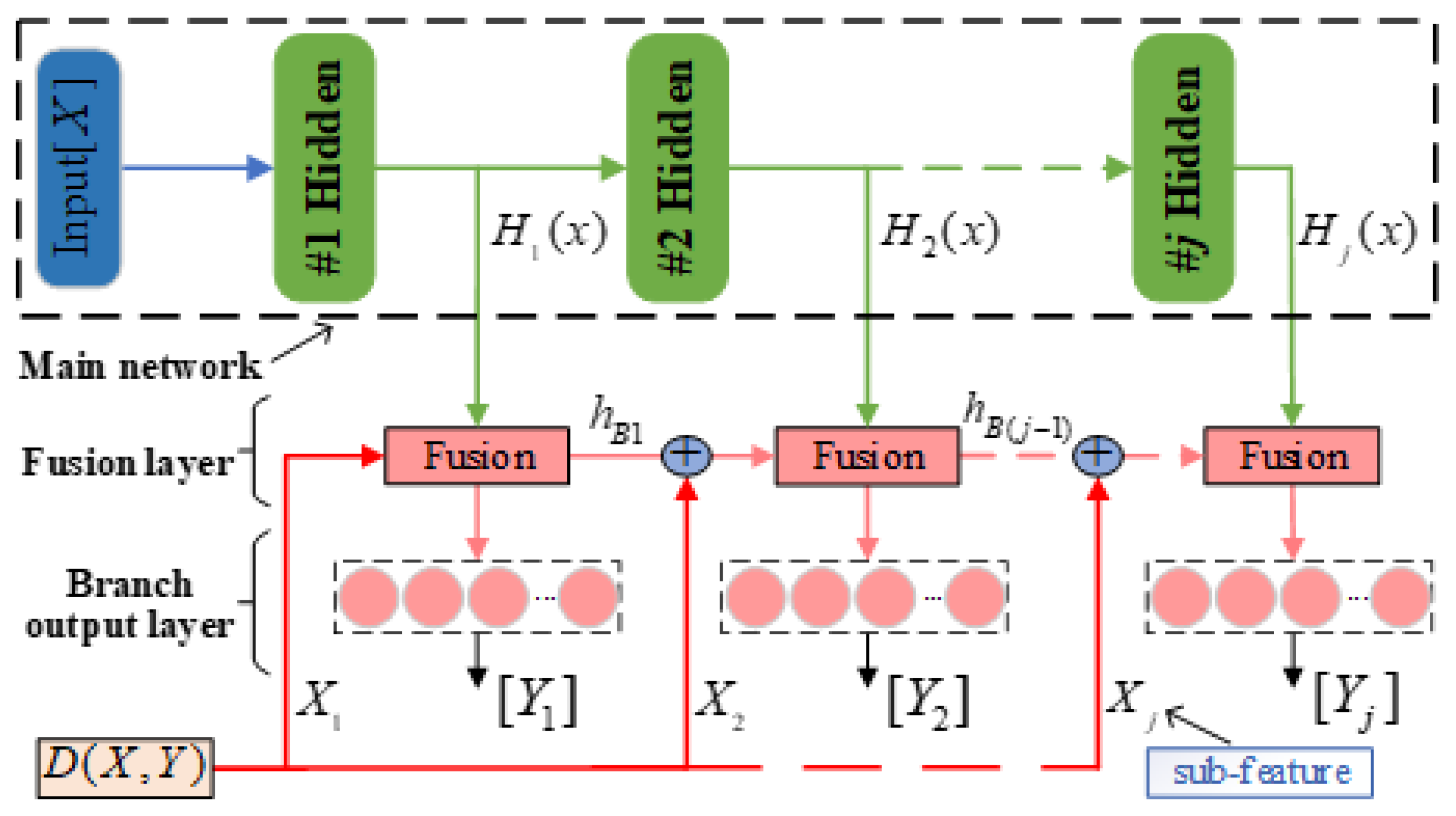
The proposed SAE-MBDFFN consists of a main network, fusion layer, and branch output layer, as shown in
Figure 4. Here,
represents the input features and
represents the actual value of the
branch. For the complex REEP, we use a multilayer structure to extract the feature information. In SAE-MBDFFN, the component content of the
extraction tank is output from the corresponding branch
, where the main network formed by stacked SAEs obtains the hidden features
of the original input based on layer-wise learning.
An actual REEP often involves dozens of extraction tanks. Supposing that the component content of each extraction tank is taken as the branch output, the resulting model will include dozens of hidden layers. This can easily result in gradient disappearance during model training [
30]. To address this, SAE-MBDFFN can solves the information loss by introducing multiscale feature fusion. Specifically, a feature fusion layer in each branch of the model extracts the residuals of the original input and the coupled features between branches.
As seen in
Figure 4, a branch is designed after each hidden layer in the main network. The branch contains the fusion layer and the output layer for result prediction. In addition to the hidden features
obtained by forward propagation, the subfeature
and coupled features
of the previous branch are also input to the fusion layer of the
branch. First, to transfer more useful information for prediction, we improve upon the traditional residual structure [
31,
32] by adding an estimate function to calculate the correlation between the original input X and branch output
. Then, a subfeature vector
that contributes more to the output is obtained, where we let
jump connects to the fusion layer of the
branch. To make the subfeatures retain more interpretable information of original features, in this paper we adopt the decision tree regression algorithm [
33] as the estimate function, expressed as follows:
Further, it is worth noting that due to the cascade relationship, there is positive coupling between adjacent extraction stages of the REEP (i.e., the component content of the previous extraction tank has an effect on the variation of the component content of the latter extraction tank). To make the model more descriptive of the actual production process, we need to consider this prior information. Thus, we design a branch feature short-connection operation for the
n+m-1 branches after branch 1. By feature short-connection, the predicted features extracted in the previous branch can be input to the fusion layer of the next branch, which is called the coupled feature between branches. The details are shown in
Figure 4, starting from the second branch fusion layer and adding another feature concatenation before each fusion layer. In this way, the j-th branch fusion layer not only possesses the deep hidden feature
of the main network and residual subfeature
input, but also the coupled features
from the previous branch.
After forward propagation, SAE-MBDFFN can simultaneously learn the original subfeatures, hidden features, and coupled features between branches in the fusion layer. Therefore, each branch of SAE-MBDFFN can use the features obtained through multiscale fusion to predict the changes in component content. The input vector (predicted feature) of the output layer of the
branch is represented as
. After realizing multiscale feature fusion, the input vector of all branch output layers can be expressed as
where
denotes the input vector of (j − 1)th branch output layer,
denotes the hidden feature of the j-th hidden layer of main network, and ⊕ represents the concatenation operator. By introducing feature fusion, the branch output function to be learned changes from
to
. This not only improves the prediction accuracy but also alleviates gradient disappearance in the deep neural network. To avoid information loss during feature transfer, in this paper we use concatenation in the feature fusion operation. Let dimensions
be r, s, t, respectively; then, the fused feature dimension obtained by the concatenation operation is
. In this way, the features of different scales can be extracted and learned simultaneously in the fusion layer of SAE-MBDFFN. The fusion features
obtained in the
branch are used for making the final prediction of the component content. For the fusion layer and output layer of branch
j, the weights and bias parameters of the connection are assumed to be
. Thus, the output expression is
, where
denotes the activation function of the output layer. Similarly, supposing
j = n + m, the output of all
n + m branches is represented as shown below.
3.2. Training Process of SAE-MBDFFN
In REEP, the component content of each extraction tank is difficult to measure in real time, and is usually obtained by offline assay. The offline assay process has a time delay, resulting in incomplete acquisition of the component content under different running conditions. However, the process feature data under different running statuses can be easily collected, which leads to a dataset with two parts: a labeled dataset , where is the number of samples, is the feature dimension (i.e., the number of input features in the sample), and represents the component content of each extraction tank, and an unlabeled dataset , which generally has due to the ease of data collection. Existing deep learning methods based on supervised training often focus only on datasets with labeled data, ignoring the larger amount of unlabeled feature data. In addition, the typical training process of deep networks adopts random initialization of parameters, which can easily lead to the network falling into local optima. To solve the shortcomings of existing training methods, we propose an unsupervised pretraining method based on stacked SAEs for the parameter initialization of SAE-MBDFFN.
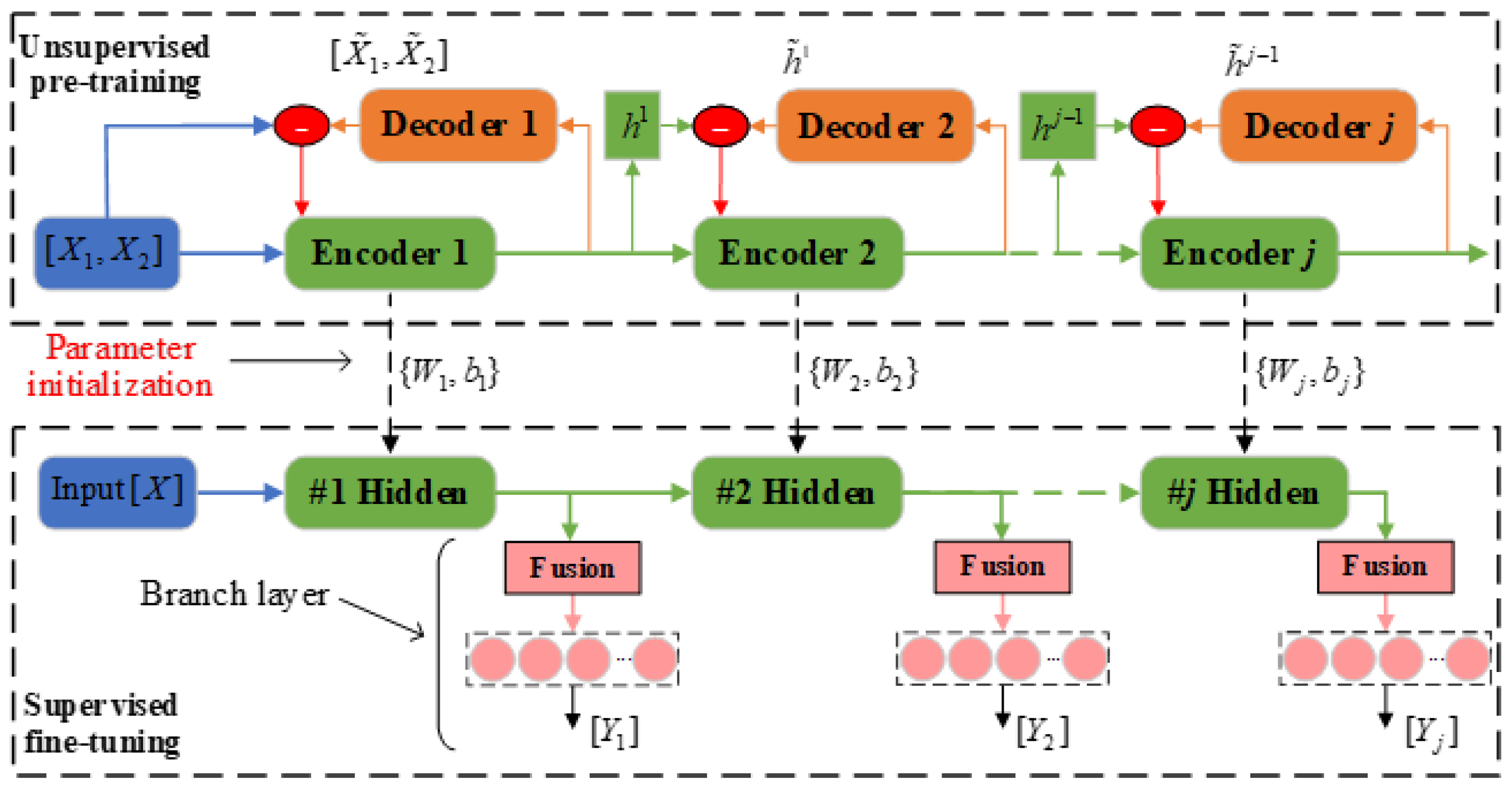
The complete training procedure of SAE-MBDFFN is shown in
Figure 5. We define it in two stages: an unsupervised pretraining process using only feature data, and a supervised fine-tuning process using labeled data. In the pretraining stage, a stacked SAE network is constructed with the same number of layers as the SAE-MBDFFN main network. Then, unsupervised training of the stacked SAE uses the feature dataset
. The first SAE structure consists of the input, encoder 1, and decoder 1 layers. First, encoder 1 learns the hidden representation of the input features and outputs its reconstruction
to decoder 1. The output vector of encoder 1 is denoted as
. Then, decoder 2 outputs its reconstruction
obtained by feature extraction to encoder 2. The subsequent process is similar to this. For a deep SAE structure with a total of n+m encoders, the latter SAE reconstructs the encoder output of the previous SAE by minimizing the sparse loss function
. In this way, training proceeds layer-wise until the
SAE, obtaining a multilayer representation of the original input.
The pretraining process of SAE-MBDFFN does not require labeled data, and hidden information can be learned through the error backpropagation algorithm. After the pretraining, the weight matrix and bias vector parameters of each encoder are expressed as
. For convenience of display, in
Figure 5 we refer to the fusion layer and branch output layer of SAE-MBDFFN together as the branch layer.
After unsupervised pretraining is completed, supervised fine-tuning is carried out. For the stacked SAE network, we remove its decoder parts and retain the (
n + m) stacked encoders as the main network of SAE-MBDFFN. On this basis, the SAE-MBDFFN model can be constructed by introducing the branch output after each encoder. The encoder parameter
obtained during pretraining is the initial parameter of the main network. The labeled dataset
is then used to fine-tune the whole network. The fine-tuning process needs to first establish the objective loss function of each branch output. In this paper, the MSE function is adopted. For SAE-MBDFFN with branch output, the loss function is represented as follows.
In the above equation
,
is the loss function of the
branch, where N is the total number of training samples,
is the actual value of the
branch output, and
is the predicted output of the corresponding branch; moreover,
denotes the cumulative weight matrix and bias vector of input to
branch. To update the network parameters
during the fine-tuning stage, this paper uses the Adam algorithm [
16] for iterative training.
3.3. SAE-MBDFFN-Based REEP Simulation
The SAE-MBDFFN method proposed in this paper simulates complex REEPs with strong coupling and multiple outputs through innovative design of a multi-branch structure and multiscale feature fusion mechanism. Further, a pretraining method based on stacked SAEs enables the model to obtain initial parameter values that conform to the actual feature distribution. The training method effectively uses a large amount of unlabeled data while avoiding the shortcomings around local optima encountered with random parameter initialization.
There are four main steps in SAE-MBDFFN-based REEP modeling. First, original data are collected and preprocessed. Second, a stacked SAE network matched with the main network of SAE-MBDFFN is established and the SSAE undergoes layer-wise unsupervised learning via backpropagation. In this step, each encoder can learn the hidden representation of the original feature. Third, the decoder parts of the SSAE network are discarded and the encoder parts are stacked to construct the main network of SAE-MBDFFN, then supervised fine-tuning is performed on the whole model to update all parameters. Lastly, component content is output in each branch layer for the testing samples by substituting only their raw input data into the trained SAE-MBDFFN network and then carrying out forward propagation. The details of the REEP simulation are as follows:
- (1)
The feature data and corresponding labeled data are collected as the original dataset, where denotes the component content of the organic and aqueous phases in the extraction stage. Then, the network structure of SAE-MBDFFN is determined according to the actual REEP.
- (2)
Unsupervised pretraining of the main SAE-MBDFFN network is performed. First, the initial SAE is trained to minimize the reconstruction error between the input data and reconstructed data . Then, the parameter set of the first encoder and the hidden feature representation can be obtained, where L represents the number of neurons.
- (3)
In a similar way, pretraining of the stacked SAE network is completed by reconstructing the previous encoder’s output in a layer-wise manner. The obtained weight and bias parameter set are then used the initial parameters of the main network.
- (4)
After determining the initial parameters of the main network, the whole SAE-MBDFFN network is fine-tuned based on the labeled dataset . The loss function corresponding to the output of each branch is constructed, and the Adam algorithm is used to continuously minimize the output prediction error , . When the loss function converges to around zero, the optimal model in the process is saved and the fine-tuning is considered complete.
- (5)
Finally, the model’s prediction accuracy can be evaluated using test data. If the model meets accuracy requirements, it can achieve the purpose of simulating REEP, with the branch output being the component content.


