Rate Transient Analysis for Fractured Wells in Inter-Salt Shale Oil Reservoirs Considering Threshold Pressure Gradient

Abstract

The low-velocity non-Darcy effect within the shale matrix significantly influences the well production performance of shale reservoirs, primarily caused by the threshold pressure gradient identified by various researchers. Moreover, in inter-salt shale reservoirs, salt minerals dissolve and diffuse when they encounter water-based working fluids, resulting in substantial alterations in pore structure. This paper introduces a transient pressure model for inter-salt shale oil reservoirs that accounts for oil flow from formation to the wellbore, considering all of the aforementioned mechanisms. The partial differential equations of this dual-porosity model, which incorporate salt dissolution and the low-velocity non-Darcy effect in the shale matrix, are derived. An accurate solution is achieved through the application of Laplace transformation and Green’s functions. We derive the analytical solutions for transient pressure and production in real space by employing the Stehfest numerical inversion method and obtain the bi-logarithmic type curves. Six distinct flow regimes are identified, and the impacts of salt dissolution, the threshold pressure gradient, the cross-flow coefficient, and the storativity ratio are discussed. This analysis holds significant importance for evaluating fluid flow and transport in inter-salt shale oil reservoirs.

1. Introduction

As the gap between the world’s energy supply and demand continues to increase, unconventional resources have received extensive worldwide attention [1], for instance, shale oil reserves. The EIA reported that the US has 59 billion barrels of technically recoverable oil resources, and nearly half of all produced crude oil comes from shale reservoirs. China is predicted to have 32 billion barrels of technically recoverable oil resources [2]. Inter-salt shale formation is regarded as a high-quality source rock among shale reservoirs, because the oil produced in inter-salt shales is effectively trapped within the formation, owing to the barrier created by the upper and lower salt layers. The Jianghan Basin, as a typical salt lake basin in the eastern fault depression, has rich shale oil resources in the Qianjiang Sag, which is one of the areas with the best development conditions of salt lake shale oil in China [3]. However, the development process of inter-salt shale oil reservoirs differs from that of other oil fields because of its significant salt content, which encourages researchers to investigate the oil flow mechanisms behind the phenomenon in inter-salt shale reservoirs.

The high salt mineral content in inter-salt shale oil reservoirs results in the relatively high solubility of these salts. When the salt minerals come into contact with water-based working fluids, processes such as dissolution and diffusion take place. Additionally, changes in temperature and pressure can cause recrystallization of the dissolved salts, which can significantly affect the pore structure of the reservoir. Researchers have indeed found that salt dissolution significantly affects shale permeability through various laboratory experiments. Yang et al. examined the alterations in the pore structure resulting from salt dissolution by analyzing scanning electron microscopy (SEM) images of shale samples soaked in water [4]. Zhang et al. observed that salt precipitation significantly affects flow performance, with salt potentially causing damage to core permeability of over 90% [5]. Li et al. investigated that core permeability improved by 34.76% and 61.15% after flooding with low salinity water and ultra-pure water, respectively [6].

The low-velocity non-Darcy effect within the shale matrix is believed to be one of the factors hindering the development of shale oil reservoirs [7], which also leads to a significant decrease in ultimate recovery, as shown in previous studies [8]. Many scholars believe that the non-Darcy flow existing in low permeability reservoirs can be attributed to the threshold pressure gradient (TPG) and have investigated the flow problems related to the TPG [9,10,11,12,13,14]. Pascal [15] studied the influence of the TPG on fluid flow in porous media and evaluated its effect on pressure and flow rates. Lu and Ghedan [16] proposed various analytical solutions for the transient pressure equations related to vertical wells in low permeability reservoirs, taking the TPG into account. Numerical calculation methods have also been studied by scholars [17,18]. Song et al. [19] considered the low-velocity non-Darcy flow effect when establishing the steady productivity equations of fractured wells in tight gas reservoirs and concluded that the TPG had a great influence on the flow rate of gas wells and could not be disregarded.

Well pressure behavior analysis and transient rate decline analysis with consideration of the TPG have been applied in different types of oil and gas reservoirs [20,21,22,23,24,25,26], However, there is no literature that presents the transient pressure model for fractured wells in the inter-salt shale oil reservoir. In this paper, the mathematical model of fractured wells in the inter-salt shale oil reservoir is derived and the exact solution of this model is obtained by applying the Laplace transform, the Bessel equation, and Green’s functions. The analytical solutions for transient pressure and production in real space are derived by employing the Stehfest numerical inversion algorithm. This study addresses how factors such as the TPG, salt dissolution, the cross flow coefficient, and the storativity ratio influence the type curves of transient pressure and rate decline behaviors of a fractured well in an inter-salt shale oil reservoir.

2. Mathematical Model

Figure 1 shows the schematic of a fractured well produced in an inter-salt shale oil reservoir. The inter-salt shale oil reservoir can be characterized as dual-porosity media including a matrix system and a fracture system with relatively independent physical properties. Given a physical model of a fractured vertical well produced in an inter-salt shale oil reservoir (as illustrated in Figure 1), oil first flows from the fracture system to the fractured well. When the pressure in the fracture system decreases, oil stored in the matrix system begins to flow into the fracture system.

To make this mathematical model easier to solve, it is necessary to make certain assumptions to derive the analytical solutions for complex flow equations:

(1)

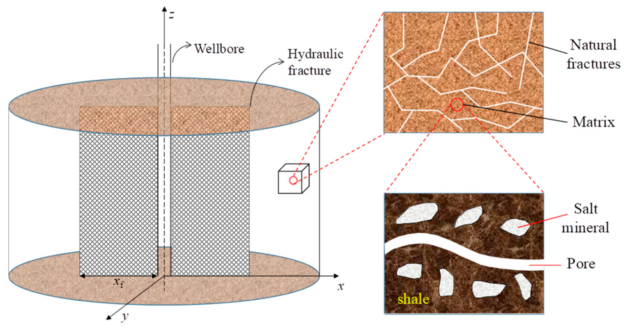
The inter-salt shale oil reservoir is treated as the dual-porosity system, while the matrix is considered to be a uniformly distributed gas source that supplies gas to the fracture system, and gas does not flow from the matrix system to the wellbore directly;

(2)

The reservoir is assumed to be isotropic. The lateral boundary extends infinitely, and the top and bottom boundaries are not permeable.

(3)

The fractured well is produced at a constant wellbore pressure or a constant rate, and hydraulic fractures are fully penetrated and have infinite conductivity;

(4)

The skin effect and wellbore storage effect are considered;

(5)

Oil flow in the inter-salt shale oil reservoir is under isothermal conditions.

2.1. Dimensionless Mathematical Model

The mathematical model of a fractured vertical well in the inter-salt shale oil reservoir, considering the TPG, is shown in Appendix A.

The dimensionless variables definitions are outlined as follows:

$$p_{\mathrm{fD}}={\displaystyle \frac{K_{\mathrm{f}}h\left(p_{\mathrm{i}}-p_{\mathrm{f}}\right)}{q_{\mathrm{sc}}B\mu }}$$

(1)

$$p_{\mathrm{mD}}={\displaystyle \frac{K_{\mathrm{mi}}h\left(p_{\mathrm{i}}-p_{\mathrm{m}}\right)}{q_{\mathrm{sc}}B\mu }}$$

(2)

$${\lambda }_{BD}={\displaystyle \frac{K_{\mathrm{f}}hL}{q_{\mathrm{sc}}B\mu }}{\lambda }_B$$

(3)

$$t_D={\displaystyle \frac{K_{\mathrm{f}}t}{\left({\varphi }_{\mathrm{f}}{C}_{\mathrm{ft}}+{\varphi }_{\mathrm{m}}{C}_{\mathrm{mt}}\right)\mu L^2}}$$

(4)

$$C_{\mathrm{D}}={\displaystyle \frac{C}{\left({\varphi }_{\mathrm{f}}{C}_{\mathrm{ft}}+{\varphi }_{\mathrm{m}}{C}_{\mathrm{mt}}\right)h{L}^2}}$$

(5)

$$\omega ={\displaystyle \frac{{\varphi }_{\mathrm{f}}{C}_{\mathrm{ft}}}{{\varphi }_{\mathrm{f}}{C}_{\mathrm{ft}}+{\varphi }_{\mathrm{m}}{C}_{\mathrm{mt}}}}$$

(6)

$$\lambda =\alpha {\displaystyle \frac{K_{\mathrm{mi}}-F}{K_{\mathrm{f}}}}{L}^2$$

(7)

$$r_{\mathrm{D}}={\displaystyle \frac{r}{L}}$$

(8)

Conducting the dimensionless process on Equation (A10) with the definitions of dimensionless variables, the dimensionless governing differential equations can be obtained as follows:

$$\mathrm{For} \mathrm{the} \mathrm{fracture}, {\displaystyle \frac{1}{r_{\mathrm{D}}}}{\displaystyle \frac{\partial }{\partial r_{\mathrm{D}}}}\left[r_{\mathrm{D}}{\displaystyle \frac{\partial p_{\mathrm{fD}}}{\partial r_{\mathrm{D}}}}\right]+{\displaystyle \frac{{\lambda }_{BD}}{r_{\mathrm{D}}}}=\omega {\displaystyle \frac{\partial p_{\mathrm{fD}}}{\partial t_D}}+\left(1-\omega \right){\displaystyle \frac{\partial p_{\mathrm{mD}}}{\partial t_D}}$$

(9)

$$\mathrm{For} \mathrm{the} \mathrm{matrix}, \left(1-\omega \right){\displaystyle \frac{\partial p_{\mathrm{mD}}}{\partial t_D}}+\lambda \left(p_{\mathrm{mD}}-p_{\mathrm{fD}}\right)=0$$

(10)

For the initial condition,

$${\left.p_{\mathrm{fD}}\right|}_{t_{\mathrm{D}}=0}={\left.p_{\mathrm{mD}}\right|}_{t_{\mathrm{D}}=0}=0$$

(11)

For the inner boundary condition,

$$\underset{r_{\mathrm{D}}\to 0}{\lim }\left[r_{\mathrm{D}}\left({\displaystyle \frac{\partial p_{\mathrm{fD}}}{\partial r_{\mathrm{D}}}}+{\lambda }_{\mathrm{BD}}\right)\right]=-1$$

(12)

For the infinite lateral boundary condition,

$${\left.p_{\mathrm{fD}}\right|}_{r_{\mathrm{D}}\to \infty }={\left.p_{\mathrm{mD}}\right|}_{r_{\mathrm{D}}\to \infty }=0$$

(13)

2.2. Solution to Mathematical Model

Considering the nonlinearity of the seepage differential Equation (9), the Laplace transform is implemented with respect to time, the seepage differential equation is degenerated to the Bessel equation, and Green’s functions are combined to derive the exact solution of the model.

Taking the following Laplace transformation,

$${\overline{p}}_{\mathrm{D}}={\displaystyle {\int }_0^{+\infty }{p}_{\mathrm{D}}{\mathrm{e}}^{-s{t}_{\mathrm{D}}}}\mathrm{d}t$$

(14)

where s represents the variable of the Laplace transform.

Applying the Laplace transform to Equations (9)–(13) with respect to t_D, we can obtain the following:

$${\displaystyle \frac{1}{r_{\mathrm{D}}}}{\displaystyle \frac{\partial }{\partial r_{\mathrm{D}}}}\left(r_{\mathrm{D}}{\displaystyle \frac{\partial {\overline{p}}_{\mathrm{fD}}}{\partial r_{\mathrm{D}}}}\right)+{\displaystyle \frac{{\lambda }_{BD}}{s{r}_{\mathrm{D}}}}=\omega s{\overline{p}}_{\mathrm{fD}}+\left(1-\omega \right)s{\overline{p}}_{\mathrm{mD}}$$

(15)

$${\overline{p}}_{\mathrm{mD}}={\displaystyle \frac{\lambda }{\lambda +\left(1-\omega \right)s}}{\overline{p}}_{\mathrm{fD}}$$

(16)

$$\underset{r_{\mathrm{D}}\to 0}{\lim }\left[r_{\mathrm{D}}\left({\displaystyle \frac{\partial {\overline{p}}_{\mathrm{fD}}}{\partial r_{\mathrm{D}}}}+{\displaystyle \frac{{\lambda }_{\mathrm{BD}}}{s}}\right)\right]=-{\displaystyle \frac{1}{s}}$$

(17)

$${\left.{\overline{p}}_{\mathrm{fD}}\right|}_{r_{\mathrm{D}}\to \infty }={\left.{\overline{p}}_{\mathrm{mD}}\right|}_{r_{\mathrm{D}}\to \infty }=0$$

(18)

When $u={\displaystyle \frac{\lambda +s\omega \left(1-\omega \right)}{\lambda +\left(1-\omega \right)s}}s$, Equations (15) and (16) can be integrated as follows:

$${\displaystyle \frac{1}{r_{\mathrm{D}}}}{\displaystyle \frac{\partial }{\partial r_{\mathrm{D}}}}\left(r_{\mathrm{D}}{\displaystyle \frac{\partial {\overline{p}}_{\mathrm{fD}}}{\partial r_{\mathrm{D}}}}\right)+{\displaystyle \frac{{\lambda }_{BD}}{s{r}_{\mathrm{D}}}}-u{\overline{p}}_{\mathrm{fD}}=0$$

(19)

(1)

When λ_BD is equal to 0, both sides of Equation (19) are multiplied by $r_{\mathrm{D}}^2$:

$$r_{\mathrm{D}}^2{\displaystyle \frac{{\partial }^2{\overline{p}}_{\mathrm{fD}}}{\partial r_{\mathrm{D}}^2}}+r_{\mathrm{D}}{\displaystyle \frac{\partial {\overline{p}}_{\mathrm{fD}}}{\partial r_{\mathrm{D}}}}-u{r}_{\mathrm{D}}^2{\overline{p}}_{\mathrm{fD}}=0$$

(20)

When $x=r_{\mathrm{D}}\sqrt{u}$, and thus $r_{\mathrm{D}}={\displaystyle \frac{x}{\sqrt{u}}}$, according to the derivative rule of the composition function, Equation (20) can be written as follows:

$$x^2{\displaystyle \frac{{\partial }^2{\overline{p}}_{\mathrm{fD}}}{\partial x^2}}+x{\displaystyle \frac{\partial {\overline{p}}_{\mathrm{fD}}}{\partial x}}-\left(x^2+{\nu }^2\right){\overline{p}}_{\mathrm{fD}}=0$$

(21)

where v is equal to 0, and v represents the order of the modified Bessel equation.

So, we can obtain the general solution of Equation (21):

$${\overline{p}}_{\mathrm{fD}}=A{I}_0\left(r_{\mathrm{D}}\sqrt{u}\right)+B{K}_0\left(r_{\mathrm{D}}\sqrt{u}\right)$$

(22)

where I₀ is the modified Bessel function of the first kind of order zero, and K₀ is the modified Bessel function of the second kind of order zero. A and B are constants.

(2)

When λ_BD is not equal to 0, Equation (15) is inhomogeneous because its free term does not equal zero. We can use Green’s functions to represent the particular solution, so the general solution can be written as follows:

$${\overline{p}}_{\mathrm{fD}}=A{I}_0\left(r_{\mathrm{D}}\sqrt{u}\right)+B{K}_0\left(r_{\mathrm{D}}\sqrt{u}\right)+{\displaystyle {\int }_0^{+\infty }G\left(r_{\mathrm{D}},\tau \right)}\mathrm{d}\tau$$

(23)

where ${\displaystyle {\int }_0^{+\infty }G\left(r_{\mathrm{D}},\tau \right)}\mathrm{d}\tau$ is Green’s function, and its expression can be written as follows:

$$G\left(r_{\mathrm{D}},\tau \right)=\left\{\begin{array}{c}{\displaystyle \frac{{\lambda }_{\mathrm{BD}}}{s}}{K}_0\left(r_{\mathrm{D}}\sqrt{u}\right)I_0\left(\tau \sqrt{u}\right)\begin{array}{c}\hspace{1em}\left(0<\tau <r_D\right)\end{array}\\ {\displaystyle \frac{{\lambda }_{\mathrm{BD}}}{s}}{K}_0\left(\tau \sqrt{u}\right)I_0\left(r_D\sqrt{u}\right)\begin{array}{c}\hspace{1em}\left(r_D<\tau <+\infty \right)\end{array}\end{array}\right.$$

(24)

Substituting Equation (23) into the inner boundary conditions, we can obtain the following:

$$\begin{array}{l}\underset{r_{\mathrm{D}}\to 0}{\lim }{r}_{\mathrm{D}}{\displaystyle \frac{\partial }{\partial r_{\mathrm{D}}}}\left(A{I}_0\left(r_{\mathrm{D}}\sqrt{\mu }\right)+B{K}_0\left(r_{\mathrm{D}}\sqrt{\mu }\right)+{\displaystyle {\int }_0^{+\infty }G\left(r_{\mathrm{D}},\tau \right)}\mathrm{d}\tau \right)\\ =\underset{r_{\mathrm{D}}\to 0}{\lim }{r}_{\mathrm{D}}\left[\begin{array}{l}{r}_{\mathrm{D}}\sqrt{\mu }A{I}_1\left(r_{\mathrm{D}}\sqrt{\mu }\right)-r_{\mathrm{D}}\sqrt{\mu }B{K}_0\left(r_{\mathrm{D}}\sqrt{\mu }\right)+{\displaystyle \frac{{\lambda }_{\mathrm{BD}}}{s}}{r}_{\mathrm{D}}\sqrt{\mu }{K}_1\left(r_{\mathrm{D}}\sqrt{\mu }\right){\displaystyle {\int }_0^{r_{\mathrm{D}}}{I}_0\left(\tau \sqrt{\mu }\right)\mathrm{d}\tau }\\ +{\displaystyle \frac{{\lambda }_{\mathrm{BD}}}{s}}{r}_{\mathrm{D}}\sqrt{\mu }{I}_1\left(r_{\mathrm{D}}\sqrt{\mu }\right){\displaystyle {\int }_{r_{\mathrm{D}}}^{+\infty }{K}_0\left(\tau \sqrt{\mu }\right)\mathrm{d}\tau }\end{array}\right]\\ =-{\displaystyle \frac{1}{s}}\end{array}$$

(25)

Based on the properties of the Bessel function, we know $\underset{x\to 0}{\lim }x{I}_1\left(x\right)\to 0$ and $\underset{x\to 0}{\lim }x{K}_1\left(x\right)\to 1$, so we can obtain the following:

$$B={\displaystyle \frac{1}{s}}$$

(26)

Then, when we substitute Equation (23) into infinite boundary condition, we obtain the following:

$$\begin{array}{l}\underset{r_{\mathrm{D}}\to \infty }{\lim }{\overline{\overline{\xi }}}_{\mathrm{D}0}=A{I}_0\left(r_{\mathrm{D}}\sqrt{\mu }\right)+{\displaystyle \frac{\cos n\pi z_{\mathrm{wD}}}{2s}}{K}_0\left(r_{\mathrm{D}}\sqrt{\mu }\right)+{\displaystyle \frac{{\lambda }_{\mathrm{BD}}}{s}}{K}_0\left(r_{\mathrm{D}}\sqrt{\mu }\right){\displaystyle {\int }_0^{r_{\mathrm{D}}}{I}_0\left(\tau \sqrt{\mu }\right)}\mathrm{d}\tau \\ +{\displaystyle \frac{{\lambda }_{\mathrm{BD}}}{s}}{I}_0\left(r_D\sqrt{\mu }\right){\displaystyle {\int }_{r_{\mathrm{D}}}^{+\infty }{K}_0\left(\tau \sqrt{\mu }\right)}\mathrm{d}\tau =0\end{array}$$

(27)

According to the properties of the Bessel function, we can conclude that $\underset{x\to \infty }{\lim }{I}_0\left(x\right)\to \infty$ and $\underset{x\to \infty }{\lim }{K}_0\left(x\right)\to 0$, so we can obtain the following:

$$A=0$$

(28)

So, the line-sink solution for the inter-salt shale oil reservoir considering the threshold pressure gradient can be written as follows:

$${\overline{p}}_{\mathrm{fD}}={\displaystyle \frac{1}{s}}{K}_0\left(r_{\mathrm{D}}\sqrt{\mu }\right)+{\displaystyle {\int }_0^{+\infty }G\left(r_{\mathrm{D}},\tau \right)}\mathrm{d}\tau$$

(29)

where $r_{\mathrm{D}}=\sqrt{{\left(x_{\mathrm{D}}-x_{\mathrm{wD}}\right)}^2+{\left(y_{\mathrm{D}}-y_{\mathrm{wD}}\right)}^2}$.

By integrating Equation (29) with respect to x_w from −x_f to x_f, the pressure response of the fractured well in the inter-salt shale oil reservoir in Laplace space can be obtained:

$${\overline{p}}_{\mathrm{wDN}}={\displaystyle {\int }_{-1}^1\left[\frac{1}{s}{K}_0\left(r_{\mathrm{D}}\sqrt{\mu }\right)+{\displaystyle {\int }_0^{+\infty }G\left(r_{\mathrm{D}},\tau \right)}\mathrm{d}\tau \right]}\mathrm{d}{x}_{\mathrm{wD}}$$

(30)

where all the dimensionless coordinates in the Y direction (y_wD, y_D) are equal to 0.

Applying the Duhamel’s theorem, the pressure response of the fractured well when considering skin factor and wellbore storage coefficient can be written as follows:

$${\overline{p}}_{\mathrm{wD}}={\displaystyle \frac{s{\overline{p}}_{\mathrm{wDN}}+S}{s+C_D{s}^2\left(s{\overline{p}}_{\mathrm{wDN}}+S\right)}}$$

(31)

The relationship between the rate and the dimensionless pressure in the Laplace space can be obtained according to the study of Van Everdingen and Hurst [27]:

$${\overline{q}}_{\mathrm{D}}={\displaystyle \frac{1}{s^2{\overline{p}}_{\mathrm{wD}}}}$$

(32)

3. Flow Behavior Characteristics

Type curves of transient pressure have attracted considerable attention from researchers [28,29,30] as they can interpret the physical property parameters of a reservoir which are not clearly understood and assist in recognizing the flow behaviors occurring in the actual reservoir. The Stehfest numerical inversion algorithm [31] is used to derive the dimensionless wellbore pressure in real space. The input parameters are detailed in

Table 1. The parameters required for simulation.

Parameters	Symbols	Values	Units
Formation pressure	pi	2.34 × 107	Pa
Formation thickness	h	10	m
Threshold pressure gradient	λB	5.2 × 104	Pa/m
Matrix permeability	km	2.4 × 10−19	m2
Formation thickness	h	10	m
Fracture permeability	kfh	2.0 × 10−13	m2
Fracture porosity	ϕf	0.039	dimensionless
Oil viscosity	μ	2.95 × 10−3	Pa·s
Matrix compressibility	cmt	6.2 × 10−11	1/Pa
Fracture compressibility	cft	4.3 × 10−9	1/Pa
Half-length of hydraulic fracture	xf	50	m

.

3.1. Flow Regimes Recognition

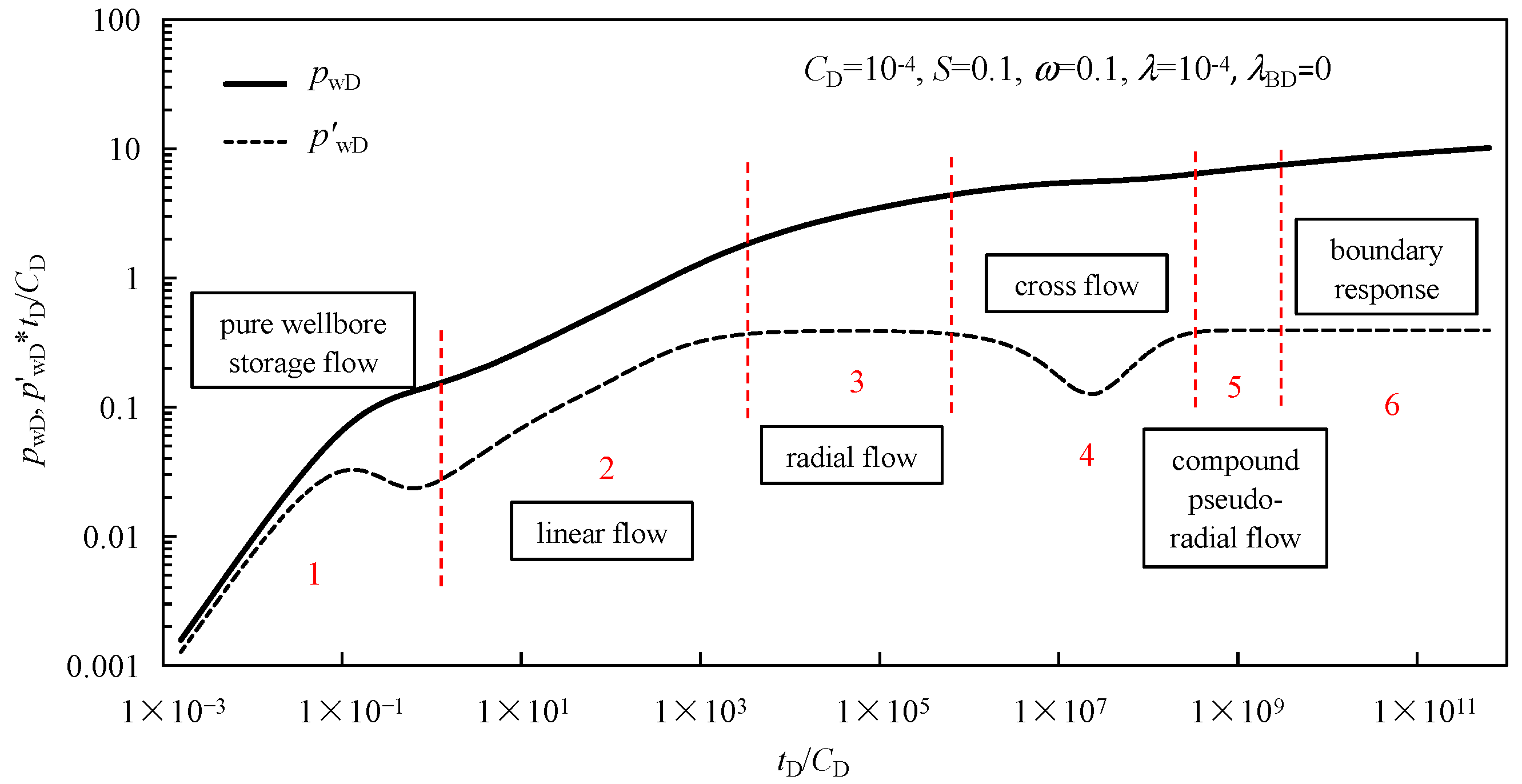
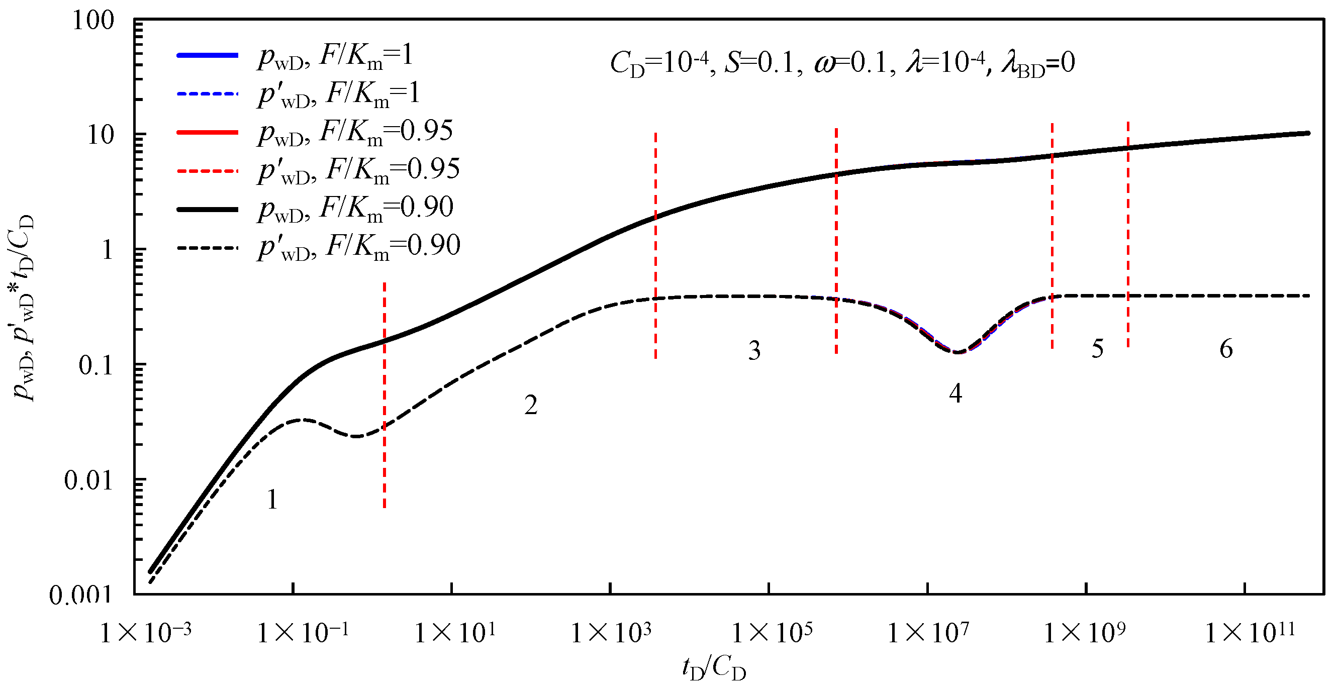
Figure 2 presents the type curves of transient pressure behavior of a fractured vertical well in the inter-salt shale oil reservoir considering the threshold pressure gradient, and six flow periods are recognized as follows:

Period 1:

The pure wellbore storage period. The pressure curve and its derivative curve are on an upward-sloping line with a slope of one, which is controlled by oil stored in the wellbore. In skin effect flow periods, an obvious “hump” appears on the derivative curve, and the height and duration of the “hump” are mainly determined by the wellbore storage coefficient and skin factor.

Period 2:

The linear flow period of hydraulic fractures. In this flow period, the pressure curve and its derivative curve are parallel to each other, and the derivative curve is an upward straight line with a slope of 0.5.

Period 3:

The radial flow period of natural fractures. During this flow period, the pressure derivative curve is represented by a horizontal line at a value of 0.5. This indicates that the flow in the natural fracture system is radial, showing consistent pressure changes over time.

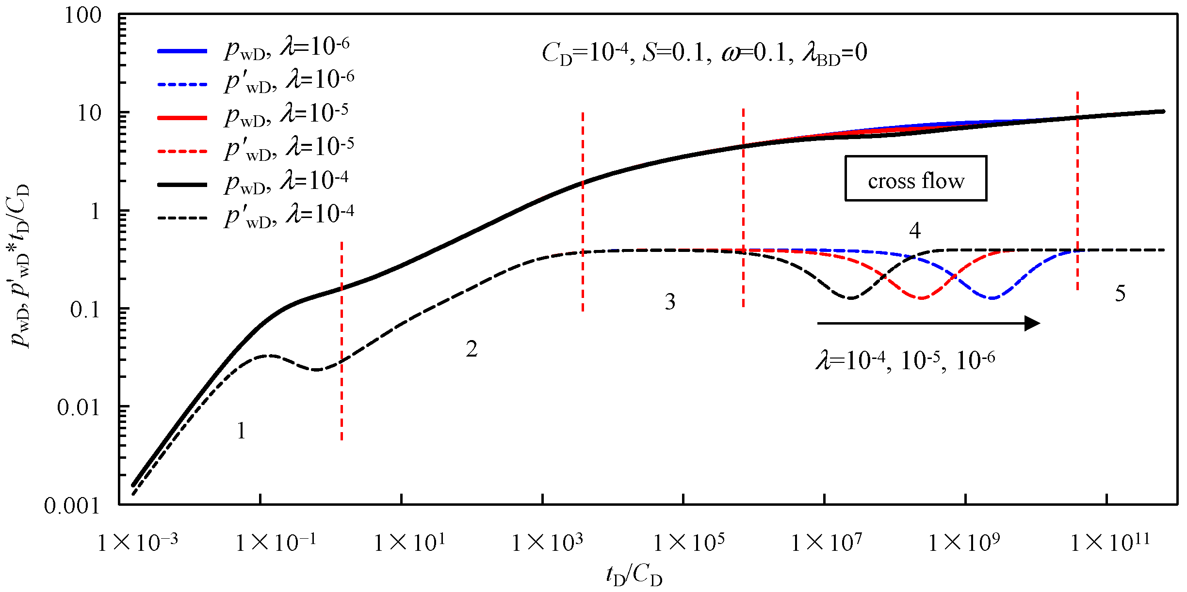
Period 4:

The cross-flow period. The most obvious characteristic of this period is the “dip” in the pressure derivative curve. In this stage, the shale oil flows from the matrix to the fracture due to the increasing pressure difference between the fracture system and the matrix system.

Period 5:

The late-time compound pseudoradial flow period. The pressure derivative curve is a horizontal line with a value of 0.5, indicating that the entire system is experiencing radial flow.

Period 6:

The external boundary response period.

3.2. Parameter Influence

Figure 3 presents the effects of the threshold pressure gradient (TPG) on dimensionless pressure and pressure derivative curves of the fractured vertical well. Beginning with Period 3 (the radial flow period of natural fractures), the influence of the threshold pressure gradient begins to appear, and the pressure curve and its derivative curve begin to deviate and warp up. Additionally, the curve will be more warped with the increase in the TPG. This is because the larger the TPG, the worse the physical properties of the reservoir, the more difficult it is for shale oil to flow, and the greater the production pressure differential required to break through the barrier of the TPG and start flow into the larger channel.

Figure 4 shows the effect of salt dissolution on transient pressure curves. Based on the experimental results of permeability affected by salt dissolution, as the average pressure reduces from 22.5 MPa to 7.5 MPa, the permeability decreases by only 5.06%. It can be found that the influence of salt dissolution on the dimensionless pressure and pressure derivative curves of the fractured vertical well can be neglected by introducing the mathematical relationship obtained from the experiment into the model.

Figure 5 presents the effect of the storativity ratio on transient pressure curves. As illustrated in the figure, the storativity ratio not only influences the cross-flow period but also affects the curve shape of the linear flow period. The smaller ω is, the deeper the “dip” is, and the higher the curve position of pressure and its derivative curves in the linear flow period. According to the definition of ω, a larger ω value indicates that more oil is stored in the fracture system. Consequently, less oil is supplied from the matrix system to the fracture system, resulting in a shallower “dip”. Additionally, more oil is supplied from the fracture system to the hydraulic fractures, which causes deeper pressure and pressure derivative curves in the linear flow period.

Figure 6 presents the influence of the cross-flow coefficient on transient pressure curves. As illustrated in the figure, the cross-flow coefficient has a significant impact on the occurrence time of the cross-flow period. The larger the cross-flow coefficient, the earlier the shale oil in the matrix system flows to the fracture system, and the earlier the “dip” on the pressure derivative pressure curve will appear.

Figure 7 presents the transient production rate curves influenced by the threshold pressure gradient. The figure shows that the larger the TPG, the greater the decline of the dimensionless production curve and the greater the upturning of its derivative curve. The reason for this is that the higher the threshold pressure gradient, the worse the physical properties of the reservoir, leading to a reduced production rate under the same pressure difference. Additionally, the existence of the threshold pressure gradient causes rapid formation energy consumption, faster production decline, and higher upturning of the production derivative curve.

Figure 8 shows the transient production rate curves affected by salt dissolution. It can be observed that the impact of salt dissolution on the dimensionless production curve of the fractured vertical well can be neglected by introducing the mathematical relationship derived from the experiment data into the model.

Figure 9 presents the transient production rate curves affected by the storativity ratio. The figure shows that the elastic storativity ratio has the most obvious influence on the middle period of the production decline curve. As the elastic storativity ratio decreases, the “dip” of the production derivative curve becomes deeper and wider. When the elastic storativity ratio becomes larger, the “dip” becomes shallower and narrower. This occurs because the larger the storativity ratio is, the stronger the storage capacity of the natural fracture system is, the more fluid is stored, the more oil is produced by the fracture system under the same differential pressure, and the higher the position in the middle of the dimensionless production curve is. In addition, the later the cross-flow period occurs, the later the “dip” of the production derivative curve appears, the less obvious the “dip” is, and the shorter the duration is.

Figure 10 presents the transient production rate curves influenced by the cross-flow coefficient. The figure shows that the cross-flow coefficient primarily influences the appearance of the “dip” of the derivative curve. The smaller the cross-flow coefficient is, the stronger the flow capacity of the natural fracture is, leading to a greater difference between the fracture and the matrix, which makes it more challenging for the oil in the matrix to flow into the fracture. As shown in the figure, the smaller the cross coefficient is, the later the cross-flow period occurs, the lower the production is, and the later the “dip” of the production derivative curve appears.

We can see from Figure 9 and Figure 10 that the storativity ratio ω and the cross-flow coefficient affect different flow periods of the transient production rate curves. According to the definition of both parameters, a larger ω value indicates that more oil is stored in the fracture system, and consequently, more oil is supplied from the fracture system to the hydraulic fractures, which makes the production curve begin to change in Period 2 (the linear flow period of hydraulic fractures). However, the cross-flow coefficient means the ratio of the flow capacity of the matrix system and the fracture system only affects Period 4 (the cross-flow period) of the production curve.

4. Conclusions

In this paper, a multi-scale comprehensive dual porosity model for a fractured well in an inter-salt shale oil reservoir that takes into account both the salt dissolution in the shale matrix and the threshold pressure gradient is established, and the transient pressure and rate decline behaviors are analyzed. The following conclusions can be summarized:

(1)

The pressure response and its pressure derivative of a fractured vertical well in the inter-salt shale oil reservoir with consideration of the threshold pressure gradient are analyzed, and six main transient flow regimes can be observed in type curves of transient pressure.

(2)

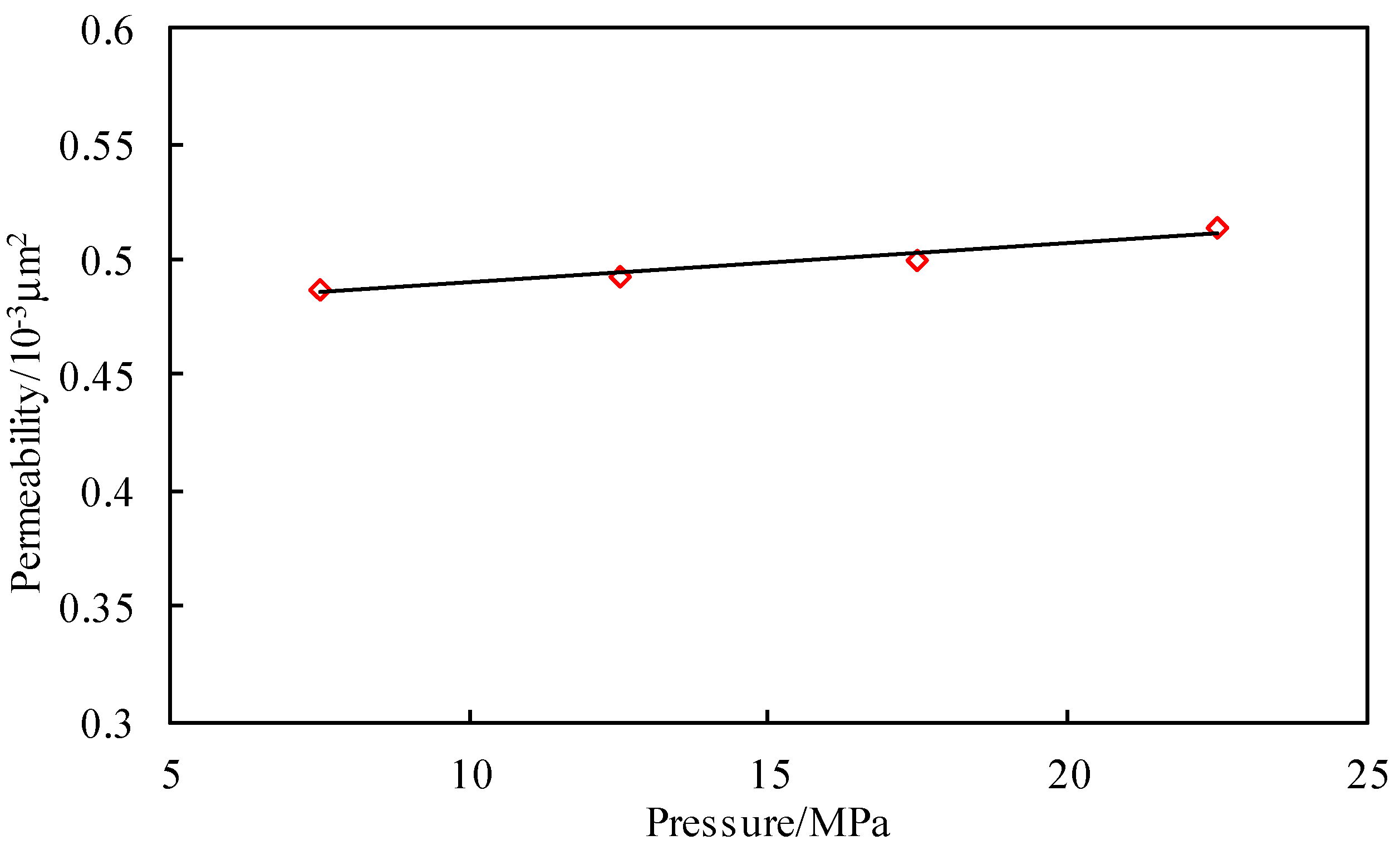
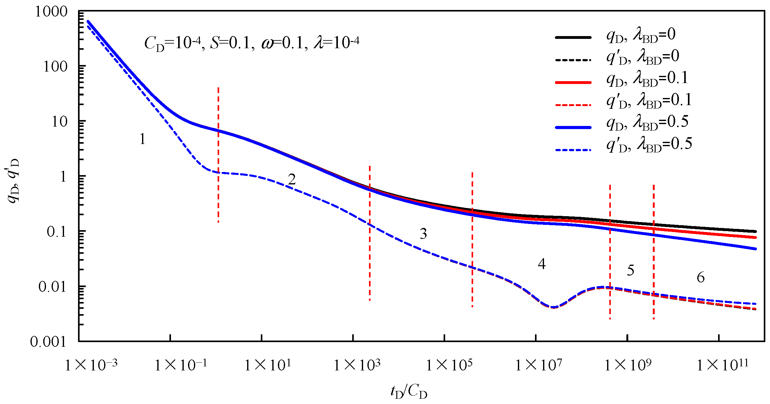
The impact of salt dissolution on the transient pressure curves and rate decline curves of a fractured well in the inter-salt shale oil reservoir is negligible based on the experimental evaluation of the effect of salt dissolution on shale permeability.

(3)

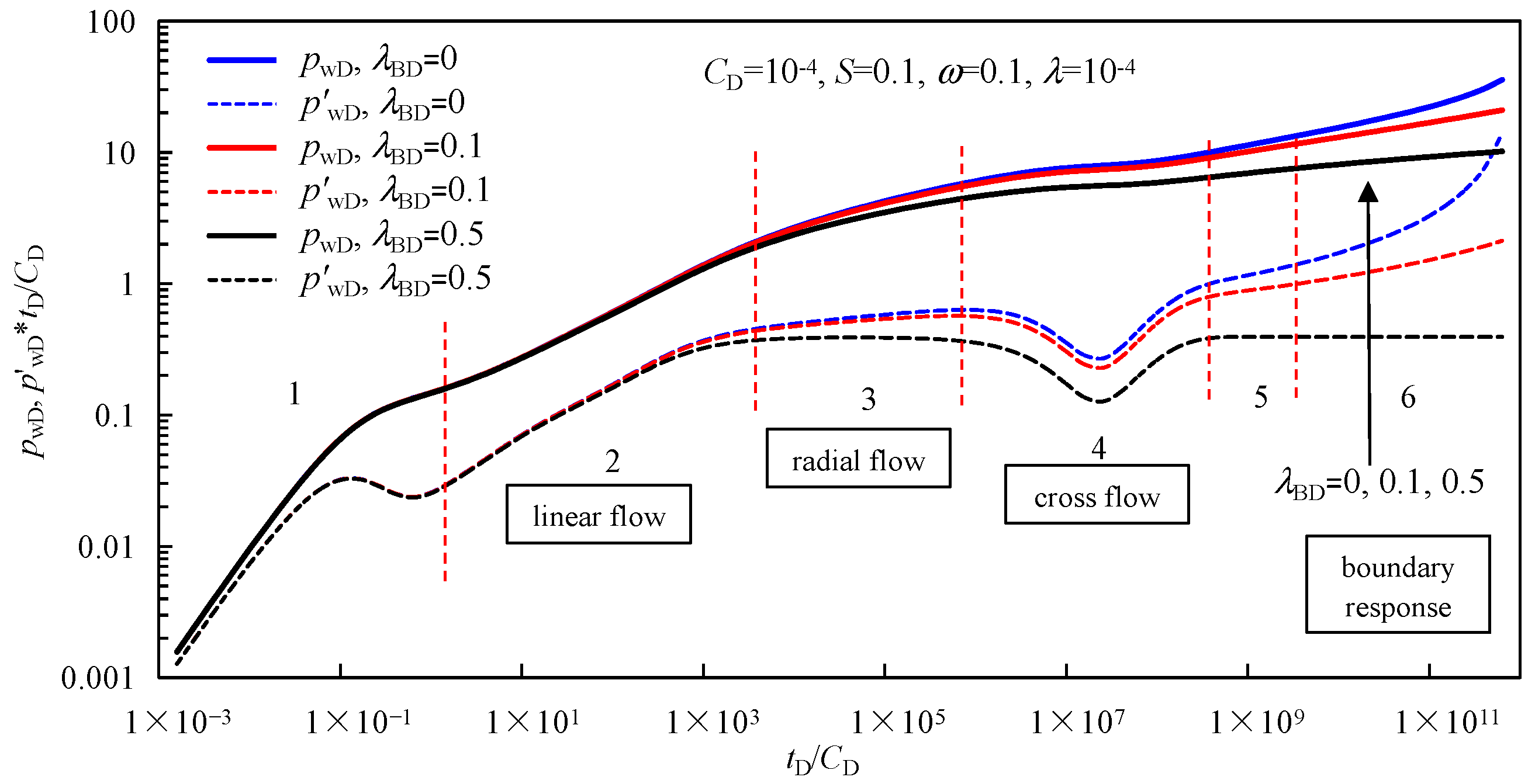
The effect of the threshold pressure gradient on the pressure derivative curves becomes apparent from the radial flow period of natural fractures (Period 3). The pressure curve and its derivative curve begin to deviate and warp up, and the curve will be more warped with the increase in the threshold pressure gradient. Type curves of rate decline curves show that the larger the threshold pressure gradient, the greater the decline of the dimensionless production curve and the greater the upturning of its derivative curve.

(4)

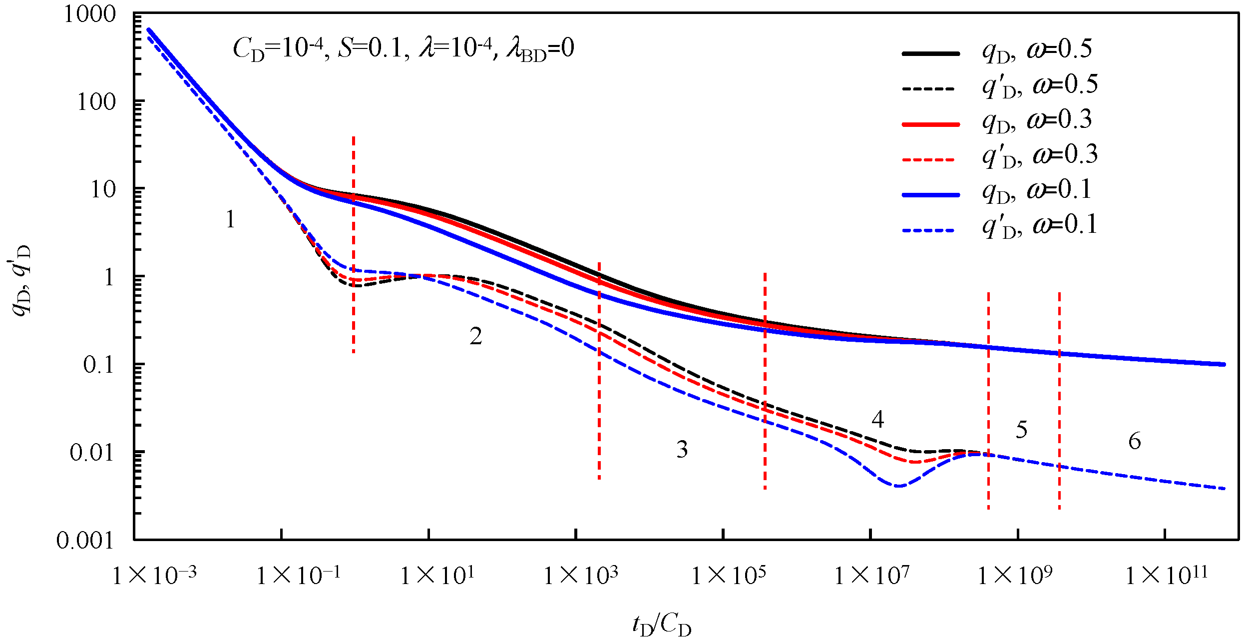
The storage capacity ratio ω not only affects the cross-flow period of pressure derivative curves but also affects the curve shape of the linear flow period, and the elastic storativity ratio has the most obvious influence on the middle period of the rate decline curves. In addition, the cross-flow coefficient also has an influence on the transient pressure and rate decline behaviors of fractured wells.

References

1. Georgeson, L.; Maslin, M.; Poessinouw, M. Clean up energy innovation. Nature 2016, 538, 27–29. [Google Scholar] [CrossRef] [PubMed]
2. Fan, X.; Su, J.Z.; Chang, X.; Huang, Z.W.; Zhou, T.; Guo, Y.T.; Wu, S.Q. Brittleness evaluation of the inter-salt shale oil reservoir in Jianghan Basin in China. Mar. Pet. Geol. 2019, 102, 109–115. [Google Scholar] [CrossRef]
3. Sun, Z.; Wang, F.; He, S.; Zheng, Y.; Wu, S.; Luo, J. The pore structures of the shale about typical inter-salt rhythm in the Paleogene of Qianjiang depression. J. Shenzhen Univ. Sci. Eng. 2019, 36, 289–297. [Google Scholar] [CrossRef]
4. Yang, L.; Lu, H.; Fan, X.; Huang, Z.; Zhou, T. Salt occurrence in matrix pores of intersalt shale oil reservoirs. Sci. Technol. Eng. 2020, 20, 1839–1845. [Google Scholar]
5. Zhang, Y.; Zhang, M.; Mei, H.; Zeng, F. Study on salt precipitation induced by formation brine flow and its effect on a high-salinity tight gas reservoir. J. Pet. Sci. Eng. 2019, 183, 106384. [Google Scholar] [CrossRef]
6. Li, Z.; Zhao, Y.; Wang, H.; Zhao, Q.; Wang, H. Effects of Injection Water Salinity on Physical Properties of Inter-Salt Shale Oil Reservoir. Spec. Oil Gas Reserv. 2020, 27, 131–137. [Google Scholar]
7. Yang, X.; Guo, B. Productivity analysis of multi-fractured shale oil wells accounting for the low-velocity non-Darcy effect. J. Pet. Sci. Eng. 2019, 183, 106427. [Google Scholar] [CrossRef]
8. Wang, X.; Sheng, J.J. Effect of low-velocity non-Darcy flow on well production performance in shale and tight oil reservoirs. Fuel 2017, 190, 41–46. [Google Scholar] [CrossRef]
9. Miller, R.J.; Low, P.F. Threshold gradient for water flow in clay system. Soil Sci. Soc. Am. J. 1963, 27, 605–609. [Google Scholar] [CrossRef]
10. Thomas, L.K.; Katz, D.L.; Tek, M.R. Threshold pressure phenomena in porous media. Soc. Petroleum Eng. J. 1968, 8, 174–184. [Google Scholar] [CrossRef]
11. Das, A.K. Generalized Darcy’s law including source effect. J. Can. Pet. Technol. 1997, 36, 57–59. [Google Scholar] [CrossRef]
12. Boukadi, F.; Bemani, A.; Rumhy, M.; Kalbani, M. Threshold pressure as a measure of degree of rock wettability and diagenesis in consolidated Omani limestone cores. Mar. Pet. Geol. 1998, 15, 33–39. [Google Scholar] [CrossRef]
13. Bennion, D.B.; Thomas, F.B.; Ma, T. Recent advances in laboratory test protocols evaluate optimum drilling, completion and stimulation practices for low permeability gas reservoirs. In Paper SPE 60324, Presented at SPE Rocky Mountain Regional/Low-permeability Reservoirs Symposium and Exhibition, Denver, CO, USA, 12–15 March 2000; SPE: Richardson, TX, USA, 2020. [Google Scholar]
14. Dey, G.R. Nonlinear flow of gas at low velocity in porous media. J. Nat. Gas Chem. 2007, 16, 217–226. [Google Scholar] [CrossRef]
15. Pascal, H. Nonsteady flow through porous media in the presence of a threshold gradient. Acta Mech. 1981, 39, 207–224. [Google Scholar] [CrossRef]
16. Lu, J.; Ghedan, S. Pressure behavior of vertical wells in low-permeability reservoirs with threshold pressure gradient. Spec. Top. Rev. Porous Media 2011, 2, 157–169. [Google Scholar] [CrossRef]
17. Wu, J.; Xu, P.; Li, L.; Li, Z.; Qi, H.; Wang, C.; Zhang, Y.; Xie, Y.; Tan, D. Multiphase dynamic interfaces and abrasive transport dynamics for abrasive flow machining in shear thickening transition states. Powder Technol. 2024, 446, 120150. [Google Scholar] [CrossRef]
18. Tan, Y.; Yesha, N.I.; Weixin, X.U.; Xie, Y.; Lin, L.I.; Tan, D. Key technologies and development trends of the soft abrasive flow finishing method. J. Zhejiang Univ.-Sci. A (Appl. Phys. Eng.) 2023, 24, 1043–1064. [Google Scholar] [CrossRef]
19. Song, H.; Liu, Q.; Yang, D.; Yu, M.; Lou, Y.; Zhu, W. Productivity equation of fractured horizontal well in a water-bearing tight gas reservoir with low-velocity non-Darcy flow. J. Nat. Gas Sci. Eng. 2014, 18, 467–473. [Google Scholar] [CrossRef]
20. Zhao, Y.; Zhang, L.; Wu, F.; Zhang, B.; Liu, Q. Analysis of horizontal well pressure behavior in fractured low permeability reservoirs with consideration of the threshold pressure gradient. J. Geophys. Eng. 2013, 10, 035014. [Google Scholar] [CrossRef]
21. Cao, L.; Li, X.; Luo, C.; Yuan, L.; Zhang, J.; Tan, X. Horizontal well transient rate decline analysis in low permeability gas reservoirs employing an orthogonal transformation method. J. Nat. Gas Sci. Eng. 2016, 33, 703–716. [Google Scholar] [CrossRef]
22. Cao, L.; Li, X.; Zhang, J.; Luo, C.; Tan, X. Dual-porosity model of rate transient analysis for horizontal well in tight gas reservoirs with consideration of threshold pressure gradient. J. Hydrodyn. 2018, 30, 872–881. [Google Scholar] [CrossRef]
23. Diwu, P.; Liu, T.; You, Z.; Jiang, B.; Zhou, J. Effect of low velocity non-Darcy flow on pressure response in shale and tight oil reservoirs. Fuel 2018, 216, 398–406. [Google Scholar] [CrossRef]
24. Zeng, J.; Wang, X.; Guo, J.; Zeng, F.; Zhang, Q. Composite linear flow model for multi-fractured horizontal wells in tight sand reservoirs with the threshold pressure gradient. J. Pet. Sci. Eng. 2018, 165, 890–912. [Google Scholar] [CrossRef]
25. Luo, E.; Wang, X.; Hu, Y.; Wang, J.; Liu, L. Analytical solutions for non-Darcy transient flow with the threshold pressure gradient in multiple-porosity media. Math. Probl. Eng. 2019, 2019, 2618254. [Google Scholar] [CrossRef]
26. Wu, Z.; Cui, C.; Lv, G.; Bing, S.; Cao, G. A multi-linear transient pressure model for multistage fractured horizontal well in tight oil reservoirs with considering threshold pressure gradient and stress sensitivity. J. Pet. Sci. Eng. 2019, 172, 839–854. [Google Scholar] [CrossRef]
27. Van Everdingen, A.F.; Hurst, W. The application of the Laplace transformation to flow problems in reservoirs. Trans. AIME 1949, 186, 97–104. [Google Scholar] [CrossRef]
28. Bumb, A.C.; McKee, C.R. Gas-well testing in the presence of desorption for coalbed methane and devonian shale. SPE Form. Eval. 1988, 3, 179–185. [Google Scholar] [CrossRef]
29. Zhan, H.; Zlotnik, V.A. Groundwater flow to horizontal and slanted wells in unconfined aquifers. Wat. Resour. Res. 2002, 38, 1108. [Google Scholar] [CrossRef]
30. Zhao, Y.; Zhang, L.; Zhao, J.; Luo, J.; Zhang, B. “Triple porosity” modeling of transient well test rate decline analysis for multi-fractured horizontal well in shale gas reservoirs. J. Pet. Sci. Eng. 2013, 110, 253–261. [Google Scholar] [CrossRef]
31. Stehfest, H. Algorithm 368: Numerical inversion of Laplace transforms. Commun. ACM 1970, 13, 47–49. [Google Scholar] [CrossRef]
Figure 1. A schematic of a fractured well in the inter-salt shale oil reservoir.
Processes 12 02833 g001
Figure 2. Log–log plots of dimensionless pressure and pressure derivatives of a fractured well in the inter-salt shale oil reservoir.
Processes 12 02833 g002
Figure 3. The effect of the threshold pressure gradient on transient pressure curves.
Processes 12 02833 g003
Figure 4. The effect of salt dissolution on transient pressure curves.
Processes 12 02833 g004
Figure 5. The effect of the storativity ratio on transient pressure curves.
Processes 12 02833 g005
Figure 6. The effect of the cross-flow coefficient on transient pressure curves.
Processes 12 02833 g006
Figure 7. The effect of the threshold pressure gradient on transient production rate curves.
Processes 12 02833 g007
Figure 8. The effect of salt dissolution on transient production rate curves.
Processes 12 02833 g008
Figure 9. The effect of the storativity ratio on transient production rate curves.
Processes 12 02833 g009
Figure 10. The effect of the cross flow coefficient on transient production rate curves.
Processes 12 02833 g010