
Coordinated Dispatch of Power Generation and Spinning Reserve in Power Systems with High Renewable Penetration

Abstract
:1. Introduction
- (1)
- Sequential Dispatch [3,4,5,6]. The power generation of each unit is dispatched in the first place, and the spinning reserve is dispatched sequentially. This means the power generation and spinning reserve are scheduled independently. It is easy to understand and implement as the scale of the problem is relatively simple and small. However, the solution of sequential dispatch is not always economically optimized. Moreover, the difference in dispatch order will also affect the result.
- (2)
- Coordinated Dispatch [7,8,9,10,11]. Power generation and spinning reserve are dispatched and optimized at the same time. It aims to minimize the operational cost while satisfying the security and reliability constraints. As wind power installation increases, the need for reserve capacity rises greatly, which leads to the change in operation mode for some conventional units [7], some of which would be replaced by wind turbines while some would be providing reserve capacity rather than generating. Power generation and reserve supply are highly coupled and therefore should be optimized concurrently. Research into this field most focused on reserve-constrained economic dispatch, which gives out the generation scheduling [9,10,11]. The total amount of spinning reserve capacity and its allocation among units is usually not specified. However, in high renewable penetration systems, demands for spinning reserve are much more urgent and frequent. The quantification of spinning reserve requirements during different time periods would help the system operator to ensure system reliability and to cut operational costs. Thus, it is important to investigate the inner relationship between spinning reserve demand and system reliability demand.
- (1)
- The spinning reserve demand in high wind power penetration system is quantified based on reliability index: the expected load not supplied ratio (ELNSR). The forced outage rate of conventional units, load and wind power output forecast error are taken into consideration to deduce the formula which gives the quantitative relations between reserve demand and reliability requirement.
- (2)
- A coordinated dispatch model of power generation and spinning reserve is presented based on the reserve quantification formula. The model aims to minimize the total system operating cost by scheduling the power generation of each unit as well as the reserve allocation during each time period. The modified RTS-96 system is used to verify the effectiveness of the proposed model. The model is solved using CPLEX 12.2 (IBM Co., Ltd., Armonk, NY, USA).
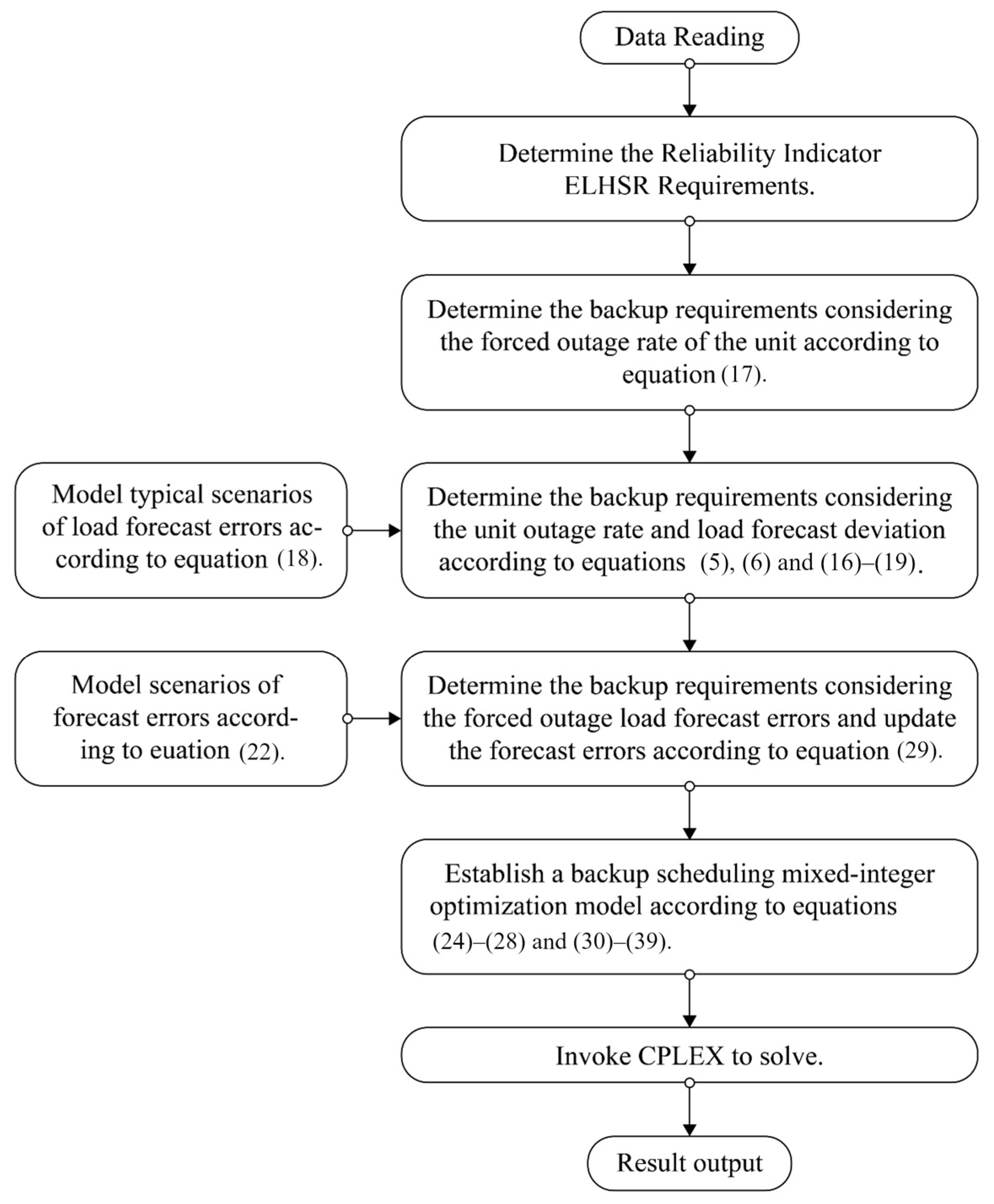
2. Quantification of Reserve Demand
2.1. Reliability Index and Reserve Demand
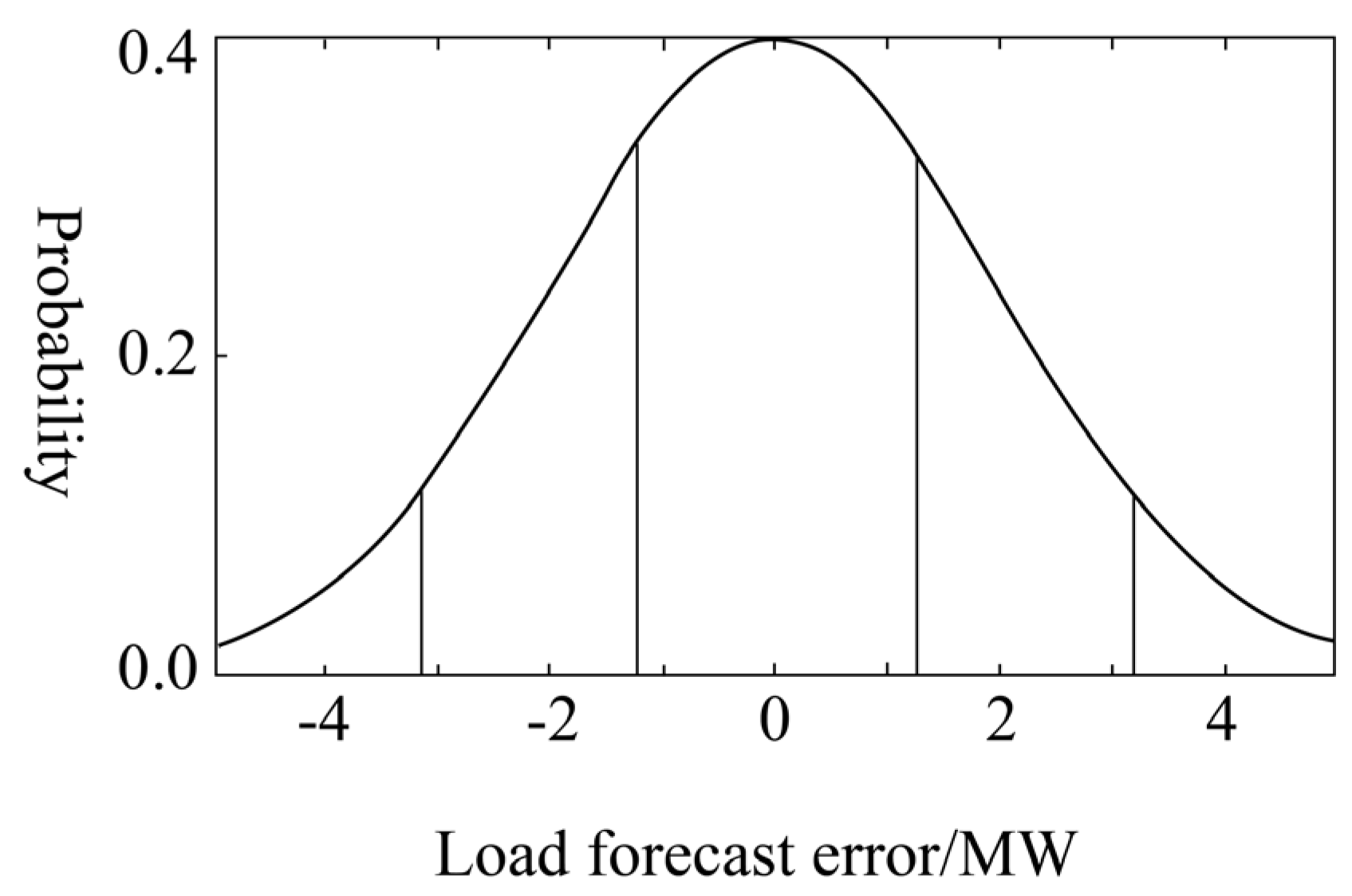
2.2. Uncertainty Description of Load
2.3. Uncertainty Description of Wind Power
3. Coordinated Generation and Spinning Reserve Dispatch Model
- (1)
- Output limits
- (2)
- Power balance limits
- (3)
- Ramp rate limits
- (4)
- Minimum up/down time limits
- (5)
- Reliability limits
4. Case Studies
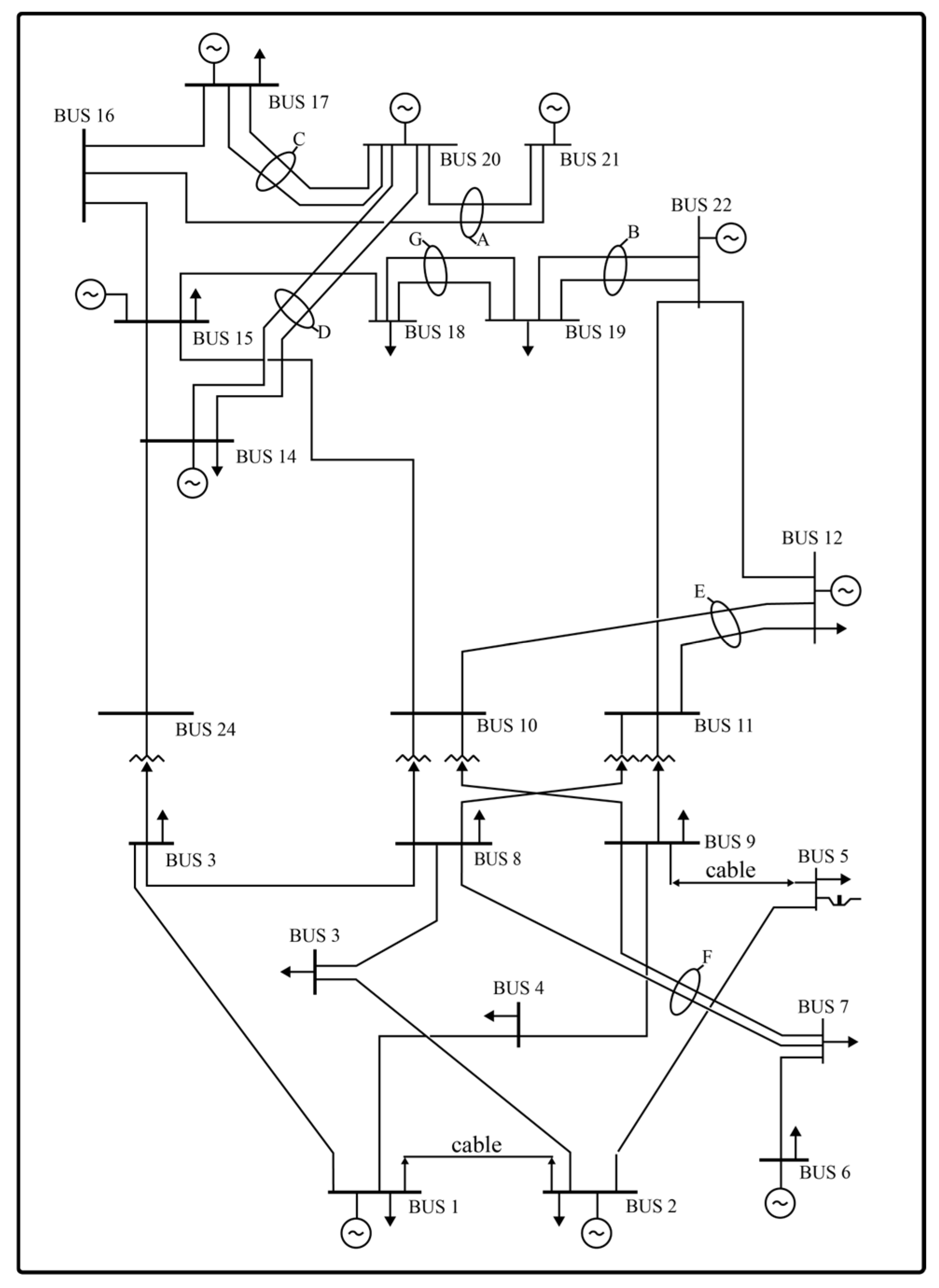
4.1. Test System
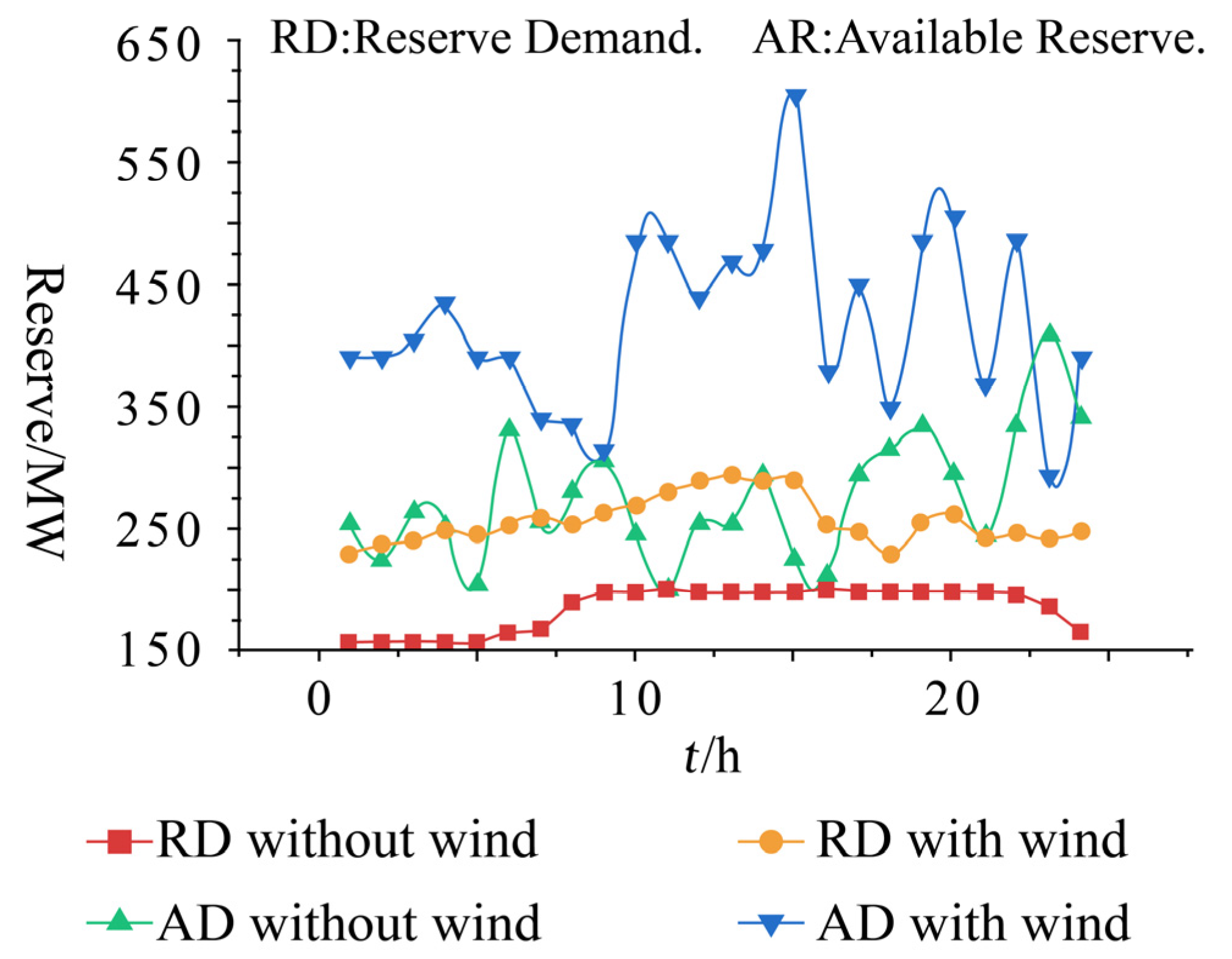
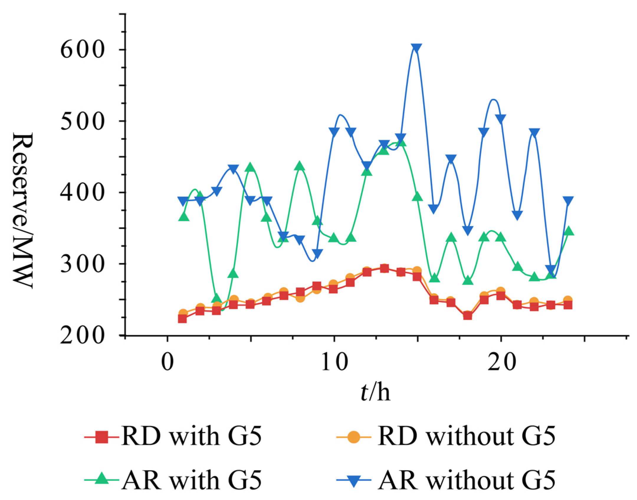
4.2. Simulation Results
5. Conclusions
Author Contributions
Funding
Data Availability Statement
Conflicts of Interest
Appendix A

| t | G1 | G2 | G3 | G4 | G5 | G6 | G7 | G8 | G9 | G1 | ||||||||||
|---|---|---|---|---|---|---|---|---|---|---|---|---|---|---|---|---|---|---|---|---|
| Output/ MW | Reserve/ MW | Output/ MW | Reserve/ MW | Output/ MW | Reserve/ MW | Output/ MW | Reserve/ MW | Output/ MW | Output/ MW | |||||||||||
| 1 | 0 | 60 | 0 | 120 | 230 | 74 | 0 | 0 | 310 | 0 | 310 | 0 | 0 | 0 | 350 | 0 | 300 | 0 | 400 | 0 |
| 2 | 0 | 60 | 0 | 120 | 260 | 44 | 0 | 0 | 310 | 0 | 310 | 0 | 0 | 0 | 350 | 0 | 300 | 0 | 400 | 0 |
| 3 | 0 | 60 | 0 | 120 | 220 | 84 | 0 | 0 | 310 | 0 | 310 | 0 | 0 | 0 | 350 | 0 | 300 | 0 | 400 | 0 |
| 4 | 0 | 60 | 0 | 120 | 230 | 74 | 0 | 0 | 310 | 0 | 310 | 0 | 0 | 0 | 350 | 0 | 300 | 0 | 400 | 0 |
| 5 | 0 | 60 | 0 | 120 | 280 | 24 | 0 | 0 | 310 | 0 | 310 | 0 | 0 | 0 | 350 | 0 | 300 | 0 | 400 | 0 |
| 6 | 0 | 60 | 0 | 120 | 304 | 0 | 76 | 151 | 310 | 0 | 310 | 0 | 0 | 0 | 350 | 0 | 300 | 0 | 400 | 0 |
| 7 | 0 | 60 | 0 | 120 | 304 | 0 | 226 | 74 | 310 | 0 | 310 | 0 | 0 | 0 | 350 | 0 | 300 | 0 | 400 | 0 |
| 8 | 56 | 4 | 0 | 120 | 304 | 0 | 300 | 0 | 310 | 0 | 310 | 0 | 300 | 155 | 350 | 0 | 300 | 0 | 400 | 0 |
| 9 | 12 | 48 | 0 | 120 | 304 | 0 | 300 | 0 | 310 | 0 | 310 | 0 | 454 | 137 | 350 | 0 | 300 | 0 | 400 | 0 |
| 10 | 0 | 60 | 0 | 120 | 304 | 0 | 300 | 0 | 310 | 0 | 310 | 0 | 526 | 65 | 350 | 0 | 300 | 0 | 400 | 0 |
| 11 | 0 | 60 | 24 | 120 | 304 | 0 | 300 | 0 | 310 | 0 | 310 | 0 | 572 | 20 | 350 | 0 | 300 | 0 | 400 | 0 |
| 12 | 0 | 60 | 0 | 120 | 304 | 0 | 300 | 0 | 310 | 0 | 310 | 0 | 516 | 75 | 350 | 0 | 300 | 0 | 400 | 0 |
| 13 | 0 | 60 | 0 | 120 | 304 | 0 | 300 | 0 | 310 | 0 | 310 | 0 | 516 | 75 | 350 | 0 | 300 | 0 | 400 | 0 |
| 14 | 0 | 60 | 0 | 120 | 304 | 0 | 300 | 0 | 310 | 0 | 310 | 0 | 476 | 115 | 350 | 0 | 300 | 0 | 400 | 0 |
| 15 | 0 | 60 | 16 | 120 | 304 | 0 | 300 | 0 | 310 | 0 | 310 | 0 | 546 | 45 | 350 | 0 | 300 | 0 | 400 | 0 |
| 16 | 0 | 60 | 0 | 120 | 304 | 0 | 300 | 0 | 310 | 0 | 310 | 0 | 560 | 31 | 350 | 0 | 300 | 0 | 400 | 0 |
| 17 | 0 | 60 | 0 | 120 | 304 | 0 | 300 | 0 | 310 | 0 | 310 | 0 | 476 | 115 | 350 | 0 | 300 | 0 | 400 | 0 |
| 18 | 0 | 60 | 0 | 120 | 304 | 0 | 300 | 0 | 310 | 0 | 310 | 0 | 456 | 135 | 350 | 0 | 300 | 0 | 400 | 0 |
| 19 | 0 | 60 | 0 | 120 | 304 | 0 | 300 | 0 | 310 | 0 | 310 | 0 | 426 | 155 | 350 | 0 | 300 | 0 | 400 | 0 |
| 20 | 0 | 60 | 0 | 120 | 304 | 0 | 300 | 0 | 310 | 0 | 310 | 0 | 476 | 115 | 350 | 0 | 300 | 0 | 400 | 0 |
| 21 | 0 | 60 | 0 | 120 | 304 | 0 | 300 | 0 | 310 | 0 | 310 | 0 | 526 | 65 | 350 | 0 | 300 | 0 | 400 | 0 |
| 22 | 0 | 60 | 0 | 120 | 304 | 0 | 300 | 0 | 310 | 0 | 310 | 0 | 406 | 155 | 350 | 0 | 300 | 0 | 400 | 0 |
| 23 | 0 | 60 | 0 | 120 | 304 | 0 | 226 | 74 | 310 | 0 | 310 | 0 | 200 | 155 | 350 | 0 | 300 | 0 | 400 | 0 |
| 24 | 0 | 60 | 0 | 120 | 295 | 9 | 75 | 151 | 310 | 0 | 310 | 0 | 0 | 0 | 350 | 0 | 300 | 0 | 400 | 0 |
| t | G1 | G2 | G3 | G4 | G5 | G6 | G7 | G8 | G9 | G1 | ||||||||||
|---|---|---|---|---|---|---|---|---|---|---|---|---|---|---|---|---|---|---|---|---|
| Output/ MW | Reserve/ MW | Output/ MW | Reserve/ MW | Output/ MW | Reserve/ MW | Output/ MW | Reserve/ MW | Output/ MW | Output/ MW | |||||||||||
| 1 | 0 | 60 | 0 | 120 | 0 | 0 | 0 | 0 | 173 | 105 | 167 | 105 | 0 | 0 | 350 | 0 | 300 | 0 | 400 | 0 |
| 2 | 0 | 60 | 0 | 120 | 0 | 0 | 0 | 0 | 158 | 105 | 152 | 105 | 0 | 0 | 350 | 0 | 300 | 0 | 400 | 0 |
| 3 | 0 | 60 | 0 | 120 | 0 | 0 | 0 | 0 | 129 | 105 | 124 | 105 | 0 | 0 | 336 | 14 | 300 | 0 | 400 | 0 |
| 4 | 0 | 60 | 0 | 120 | 0 | 0 | 0 | 0 | 120 | 105 | 115 | 105 | 0 | 0 | 306 | 44 | 300 | 0 | 400 | 0 |
| 5 | 0 | 60 | 0 | 120 | 0 | 0 | 0 | 0 | 138 | 105 | 132 | 105 | 0 | 0 | 350 | 0 | 300 | 0 | 400 | 0 |
| 6 | 0 | 60 | 0 | 120 | 0 | 0 | 0 | 0 | 173 | 105 | 167 | 105 | 0 | 0 | 350 | 0 | 300 | 0 | 400 | 0 |
| 7 | 0 | 60 | 0 | 120 | 0 | 0 | 0 | 0 | 234 | 76 | 226 | 84 | 0 | 0 | 350 | 0 | 300 | 0 | 400 | 0 |
| 8 | 0 | 60 | 0 | 120 | 300 | 4 | 120 | 151 | 310 | 0 | 310 | 0 | 0 | 0 | 350 | 0 | 300 | 0 | 400 | 0 |
| 9 | 0 | 60 | 0 | 120 | 304 | 0 | 166 | 134 | 310 | 0 | 310 | 0 | 0 | 0 | 350 | 0 | 300 | 0 | 400 | 0 |
| 10 | 0 | 60 | 0 | 120 | 304 | 0 | 86 | 151 | 310 | 0 | 310 | 0 | 200 | 155 | 350 | 0 | 300 | 0 | 400 | 0 |
| 11 | 0 | 60 | 0 | 120 | 304 | 0 | 96 | 151 | 310 | 0 | 310 | 0 | 200 | 155 | 350 | 0 | 300 | 0 | 400 | 0 |
| 12 | 0 | 60 | 0 | 120 | 200 | 104 | 0 | 0 | 310 | 0 | 310 | 0 | 200 | 155 | 350 | 0 | 300 | 0 | 400 | 0 |
| 13 | 0 | 60 | 0 | 120 | 170 | 134 | 0 | 0 | 310 | 0 | 310 | 0 | 200 | 155 | 350 | 0 | 300 | 0 | 400 | 0 |
| 14 | 0 | 60 | 0 | 120 | 160 | 144 | 0 | 0 | 310 | 0 | 310 | 0 | 200 | 155 | 350 | 0 | 300 | 0 | 400 | 0 |
| 15 | 0 | 60 | 0 | 120 | 185 | 119 | 105 | 151 | 310 | 0 | 310 | 0 | 200 | 155 | 350 | 0 | 300 | 0 | 400 | 0 |
| 16 | 0 | 60 | 0 | 120 | 304 | 0 | 256 | 44 | 310 | 0 | 310 | 0 | 200 | 155 | 350 | 0 | 300 | 0 | 400 | 0 |
| 17 | 0 | 60 | 0 | 120 | 304 | 0 | 186 | 114 | 310 | 0 | 310 | 0 | 200 | 155 | 350 | 0 | 300 | 0 | 400 | 0 |
| 18 | 0 | 60 | 0 | 120 | 304 | 0 | 286 | 14 | 310 | 0 | 310 | 0 | 200 | 155 | 350 | 0 | 300 | 0 | 400 | 0 |
| 19 | 0 | 60 | 0 | 120 | 304 | 0 | 76 | 151 | 310 | 0 | 310 | 0 | 200 | 155 | 350 | 0 | 300 | 0 | 400 | 0 |
| 20 | 0 | 60 | 0 | 120 | 285 | 19 | 115 | 151 | 310 | 0 | 310 | 0 | 200 | 155 | 350 | 0 | 300 | 0 | 400 | 0 |
| 21 | 0 | 60 | 0 | 120 | 304 | 0 | 266 | 34 | 310 | 0 | 310 | 0 | 200 | 155 | 350 | 0 | 300 | 0 | 400 | 0 |
| 22 | 0 | 60 | 0 | 120 | 304 | 0 | 116 | 151 | 310 | 0 | 310 | 0 | 200 | 155 | 350 | 0 | 300 | 0 | 400 | 0 |
| 23 | 0 | 60 | 0 | 120 | 190 | 114 | 0 | 0 | 310 | 0 | 310 | 0 | 0 | 0 | 350 | 0 | 300 | 0 | 400 | 0 |
| 24 | 0 | 60 | 0 | 120 | 0 | 0 | 0 | 0 | 183 | 105 | 178 | 105 | 0 | 0 | 350 | 0 | 300 | 0 | 400 | 0 |
References
- Rouholamini, M.; Rashidinejad, M. A Study on Scheduling of Primary Frequency Control Reserve. Int. Rev. Electr. Eng. (IREE) 2022, 7, 3628–3637. [Google Scholar]
- Yongcan, Z.; Yang, L.; Beibei, W. Impact of Two Dispatching Methods on AGC Unit Dispatch in Electricity Market Environment. Power Syst. Technol. 2020, 34, 154–159. [Google Scholar]
- Le, W.; Zhiwei, Y.; Fushuan, W. A Chance-constrained Programming Approach to Determine Requirement of Optimal Spinning Reserve Capacity. Power Syst. Technol. 2016, 30, 14–19. [Google Scholar]
- Matos, M.A.; Bessa, R.J. Setting the Operating Reserve Using Probabilistic Wind Power Forecast. IEEE Trans. Power Syst. 2023, 26, 594–603. [Google Scholar] [CrossRef]
- Wang, M.; Guo, J.; Ma, S.; Zhang, X.; Wang, T.; Luo, K. A Novel Decentralized Frequency Regulation Method of Renewable Energy Stations Based on Minimum Reserve Capacity for Renewable Energy-Dominated Power Systems. IEEE Trans. Power Syst. 2024, 39, 3701–3714. [Google Scholar] [CrossRef]
- Mota, D.D.S.; Alves, E.F.; D’Arco, S.; Sanchez-Acevedo, S.; Tedeschi, E. Coordination of Frequency Reserves in an Isolated Industrial Grid Equipped with Energy Storage and Dominated by Constant Power Loads. IEEE Trans. Power Syst. 2024, 39, 3271–3285. [Google Scholar] [CrossRef]
- Pan, C.; Shao, C.; Hu, B.; Xie, K.; Li, C.; Ding, J. Modeling the Reserve Capacity of Wind Power and the Inherent Decision-Dependent Uncertainty in the Power System Economic Dispatch. IEEE Trans. Power Syst. 2023, 38, 4404–4417. [Google Scholar] [CrossRef]
- Ortega-Vazquez, M.A.; Kirschen, D.S. Estimating the Spinning Reserve Requirements in Systems with Significant Wind Power Generation Penetration. IEEE Trans. Power Syst. 2009, 24, 114–124. [Google Scholar] [CrossRef]
- Ahmadi-Kahatir, A.; Cherkaoui, R. A Probabilistic Spinning Reserve Market Model Considering Disco’ Different Value of Lost Loads. Electr. Power Syst. Res. 2011, 81, 862–872. [Google Scholar] [CrossRef]
- Guoqiang, Z.; Wenchuan, W.; Boming, Z. Optimization of Operation Reserve Coordination Considering Wind Power Integration. Autom. Electr. Power Syst. 2011, 35, 15–19. [Google Scholar]
- Alishahi, E.; Siahi, M.; Abdollahi, A. Cost-based Unit Commitment and Generation Scheduling Considering Reserve Uncertainty Using Hybrid Heuristic Technique. Int. Rev. Electr. Eng. (IREE) 2011, 6, 379–386. [Google Scholar]
- Doherty, R.; O’Malley, M. A New Approach to Quantify Reserve Demand in Systems with Significant Installed Wind Capacity. IEEE Trans. Power Syst. 2005, 20, 587–595. [Google Scholar] [CrossRef]
- Morina, S.; Stoilov, D. Assessment of Operational Reserve Requirement Resulting from Wind Power use in the Electric Power System of Kosovo. In Proceedings of the 2023 18th Conference on Electrical Machines, Drives and Power Systems (ELMA), Varna, Bulgaria, 29 June–1 July 2023; pp. 1–4. [Google Scholar]
- Tang, Y.; Zhai, Q.; Zhou, Y. From Viewpoint of Reserve Provider: A Day-Ahead Multi-Stage Robust Optimization Reserve Provision Method for Microgrid with Energy Storage. J. Mod. Power Syst. Clean Energy 2024, 12, 1535–1547. [Google Scholar] [CrossRef]
- Hanmandlu, M.; Chauhan, B.K. Load Forecasting Using Hybrid Models. IEEE Trans. Power Syst. 2011, 26, 20–29. [Google Scholar] [CrossRef]
- Yuanzhang, S.; Jun, W.; Guojie, L. Dynamic Economic Dispatch Considering Wind Power Penetration Based on Wind Speed Forecasting and Stochastic Programming. Power Syst. Technol. 2010, 34, 163–168. [Google Scholar]
- Zhao, Y.L.; Sheng, Q.S.; Wang, J.J. Interruptible Load Included Reserve Procurement Method with Wind Power Integration. Int. Rev. Electr. Eng. (IREE) 2012, 7, 4631–4638. [Google Scholar]
- Pappala, V.S.; Erlich, I.; Rohrig, K. A Stochastic Model for the Optimal Operation of a Wind-thermal Power System. IEEE Trans. Power Syst. 2009, 24, 940–950. [Google Scholar] [CrossRef]
- Jigui, S.; Jun, S.; Guohui, X. Linearization Method of Large Scale Unit Commitment Problem with Network Constraints. Power Syst. Prot. Control 2010, 38, 135–139. [Google Scholar]
- Grigg, C.; Wong, P.; Albrecht, P. The IEEE Reliability Test System-1996, A Report Prepared by the Reliability Test System Task Force of the Application of Probability Methods Subcommittee. IEEE Trans. Power Syst. 1999, 14, 1010–1020. [Google Scholar] [CrossRef]
- Wang, C.; Shahidepour, S.M. Effects of Ramp-rate Limits on Unit Commitment and Economic Dispatch. IEEE Trans. Power Syst. 1993, 8, 1341–1350. [Google Scholar] [CrossRef]
- Bhaskar, K.; Singh, S.N. AWNN-Assisted Wind Power Forecasting Using Feed-Forward Neural Network. IEEE Trans. Power Syst. 2012, 3, 306–315. [Google Scholar] [CrossRef]
| Unit | PG,imin (MW) | PG,imax (MW) | FORi | ai (k$/MW2) | bi (k$/MW2) | ci (k$/MW2) | ||
|---|---|---|---|---|---|---|---|---|
| G1 | 12.0 | 60 | 0.02 | 0.02533 | 25.5472 | 24.3891 | ||
| G2 | 16.0 | 180 | 0.10 | 0.01199 | 37.5510 | 117.7551 | ||
| G3 | 60.8 | 304 | 0.02 | 0.00876 | 13.3272 | 81.1364 | ||
| G4 | 75 | 300 | 0.04 | 0.00623 | 18.0000 | 217.8952 | ||
| G5 | 108.5 | 310 | 0.04 | 0.00463 | 10.6940 | 142.7348 | ||
| G6 | 108.5 | 310 | 0.04 | 0.00473 | 10.7154 | 143.0288 | ||
| G7 | 206.8 | 591 | 0.05 | 0.00259 | 23.0000 | 259.1310 | ||
| G8 | 140.0 | 350 | 0.08 | 0.00153 | 10.8616 | 177.0575 | ||
| G9 | 100.0 | 400 | 0.12 | 0.00194 | 7.4921 | 310.0021 | ||
| G10 | 100.0 | 400 | 0.12 | 0.00195 | 7.5031 | 311.9102 | ||
| Unit | Ti,on (h) | Ti,off (h) | tic (h) | Init. Cond. (h) | Ch ($) | Cc ($) | PG,Ui (MW/h) | PG,Di (MW/h) |
| G1 | 0 | 0 | 0 | −1 | 60 | 30 | 60.0 | 60.0 |
| G2 | 0 | 0 | 0 | −1 | 340 | 170 | 120.0 | 160.0 |
| G3 | 3 | 2 | 2 | 3 | 60 | 30 | 154 | 300.0 |
| G4 | 4 | 2 | 2 | −3 | 840 | 420 | 151.0 | 214.0 |
| G5–G6 | 5 | 3 | 3 | 5 | 1000 | 500 | 105.0 | 148.0 |
| G7 | 5 | 4 | 4 | −4 | 4500 | 2300 | 155.0 | 299.0 |
| G8 | 8 | 5 | 5 | 10 | 4000 | 2000 | 70.0 | 120.0 |
| G9–G10 | 8 | 5 | 5 | 10 | 11,000 | 11,000 | 50.5 | 100.0 |
| T | PW,j\/ MW | t | PW,j\/ MW | t | PW,j\/ MW | t | PW,j\/ MW |
|---|---|---|---|---|---|---|---|
| 1 | 510 | 7 | 690 | 13 | 750 | 19 | 450 |
| 2 | 570 | 8 | 540 | 14 | 720 | 20 | 480 |
| 3 | 600 | 9 | 600 | 15 | 660 | 21 | 360 |
| 4 | 660 | 10 | 540 | 16 | 420 | 22 | 390 |
| 5 | 630 | 11 | 600 | 17 | 309 | 23 | 540 |
| 6 | 660 | 12 | 720 | 18 | 270 | 24 | 630 |
| T | L1/ MW | L2/ MW | L3/ MW | Total/ MW | t | L1/ MW | L2/ MW | L3/ MW | Total/ MW |
|---|---|---|---|---|---|---|---|---|---|
| 1 | 400 | 500 | 800 | 1700 | 13 | 600 | 700 | 1290 | 2590 |
| 2 | 410 | 520 | 800 | 1730 | 14 | 550 | 750 | 1250 | 2550 |
| 3 | 380 | 420 | 890 | 1690 | 15 | 600 | 800 | 1220 | 2620 |
| 4 | 400 | 500 | 800 | 1700 | 16 | 380 | 670 | 1600 | 2650 |
| 5 | 410 | 520 | 820 | 1750 | 17 | 400 | 600 | 1550 | 2550 |
| 6 | 450 | 300 | 1100 | 1850 | 18 | 310 | 520 | 1700 | 2530 |
| 7 | 500 | 400 | 1100 | 2000 | 19 | 550 | 600 | 1350 | 2500 |
| 8 | 500 | 630 | 1300 | 2430 | 20 | 540 | 610 | 1400 | 2550 |
| 9 | 640 | 500 | 1400 | 2540 | 21 | 600 | 800 | 1200 | 2600 |
| 10 | 600 | 550 | 1450 | 2600 | 22 | 630 | 750 | 1100 | 2480 |
| 11 | 380 | 590 | 1700 | 2670 | 23 | 580 | 420 | 1200 | 2200 |
| 12 | 740 | 550 | 1300 | 2590 | 24 | 400 | 540 | 900 | 1840 |
| t | G1 | G2 | G3 | G4 | G5 | G6 | G7 | G8 | G9 | G10 | ||||||||||
|---|---|---|---|---|---|---|---|---|---|---|---|---|---|---|---|---|---|---|---|---|
| Output/ MW | Reserve/ MW | Output/ MW | Reserve/ MW | Output/ MW | Reserve/ MW | Output/ MW | Reserve/ MW | Output/ MW | Reserve/ MW | Output/ MW | Reserve/ MW | Output/ MW | Reserve/ MW | Output/ MW | Reserve/ MW | Output/ MW | Output/ MW | Reserve/ MW | Output/ MW | |
| 1 | 0 | 60 | 0 | 120 | 230 | 74 | 0 | 0 | 310 | 0 | 310 | 0 | 0 | 0 | 350 | 0 | 300 | 0 | 400 | 0 |
| 6 | 0 | 60 | 0 | 120 | 304 | 0 | 76 | 151 | 310 | 0 | 310 | 0 | 0 | 0 | 350 | 0 | 300 | 0 | 400 | 0 |
| 12 | 0 | 60 | 0 | 120 | 304 | 0 | 300 | 0 | 310 | 0 | 310 | 0 | 516 | 75 | 350 | 0 | 300 | 0 | 400 | 0 |
| 18 | 0 | 60 | 0 | 120 | 304 | 0 | 300 | 0 | 310 | 0 | 310 | 0 | 456 | 135 | 350 | 0 | 300 | 0 | 400 | 0 |
| 24 | 0 | 60 | 0 | 120 | 295 | 9 | 75 | 151 | 310 | 0 | 310 | 0 | 0 | 0 | 350 | 0 | 300 | 0 | 400 | 0 |
| T | 1 | 2 | 3 | 4 | 5 | 6 | 7 | 8 | 9 | 10 | 11 | 12 | ||||||||
| Reserve Demand/MW | 156 | 156 | 156 | 156 | 156 | 165 | 168 | 190 | 198 | 198 | 200 | 198 | ||||||||
| Available Reserve/MW | 254 | 224 | 264 | 254 | 204 | 331 | 254 | 279 | 305 | 245 | 200 | 255 | ||||||||
| T | 13 | 14 | 15 | 16 | 17 | 18 | 19 | 20 | 21 | 22 | 23 | 24 | ||||||||
| Reserve Demand/MW | 198 | 198 | 198 | 200 | 198 | 198 | 198 | 198 | 198 | 196 | 185 | 165 | ||||||||
| Available Reserve/MW | 255 | 295 | 225 | 211 | 295 | 315 | 335 | 295 | 245 | 335 | 409 | 340 | ||||||||
| t | G1 | G2 | G3 | G4 | G5 | G6 | G7 | G8 | G9 | G10 | ||||||||||
|---|---|---|---|---|---|---|---|---|---|---|---|---|---|---|---|---|---|---|---|---|
| Output/ MW | Reserve/ MW | Output/ MW | Reserve/ MW | Output/ MW | Reserve/ MW | Output/ MW | Reserve/ MW | Output/ MW | Reserve/ MW | Output/ MW | Reserve/ MW | Output/ MW | Reserve/ MW | Output/ MW | Reserve/ MW | Output/ MW | Reserve/ MW | Output/ MW | Reserve/ MW | |
| 1 | 0 | 60 | 0 | 120 | 0 | 0 | 0 | 0 | 173 | 105 | 167 | 105 | 0 | 0 | 350 | 0 | 300 | 0 | 400 | 0 |
| 6 | 0 | 60 | 0 | 120 | 0 | 0 | 0 | 0 | 173 | 105 | 167 | 105 | 0 | 0 | 350 | 0 | 300 | 0 | 400 | 0 |
| 12 | 0 | 60 | 0 | 120 | 200 | 104 | 0 | 0 | 310 | 0 | 310 | 0 | 200 | 155 | 350 | 0 | 300 | 0 | 400 | 0 |
| 18 | 0 | 60 | 0 | 120 | 304 | 0 | 286 | 14 | 310 | 0 | 310 | 0 | 200 | 155 | 350 | 0 | 300 | 0 | 400 | 0 |
| 24 | 0 | 60 | 0 | 120 | 0 | 0 | 0 | 0 | 183 | 105 | 178 | 105 | 0 | 0 | 350 | 0 | 300 | 0 | 400 | 0 |
| T | 1 | 2 | 3 | 4 | 5 | 6 | 7 | 8 | 9 | 10 | 11 | 12 |
|---|---|---|---|---|---|---|---|---|---|---|---|---|
| Reserve Demand/MW | 229 | 237 | 240 | 249 | 245 | 253 | 260 | 253 | 264 | 270 | 280 | 289 |
| Available Reserve/MW | 390 | 390 | 404 | 434 | 390 | 390 | 340 | 335 | 314 | 486 | 486 | 439 |
| t | 13 | 14 | 15 | 16 | 17 | 18 | 19 | 20 | 21 | 22 | 23 | 24 |
| Reserve Demand/MW | 294 | 289 | 290 | 253 | 248 | 229 | 255 | 261 | 243 | 247 | 242 | 249 |
| Available Reserve/MW | 469 | 479 | 605 | 379 | 449 | 349 | 486 | 505 | 369 | 486 | 294 | 390 |
| t | G1 | G2 | G3 | G4 | G5 | G6 | G7 | G8 | G9 | |||||||||
|---|---|---|---|---|---|---|---|---|---|---|---|---|---|---|---|---|---|---|
| Output/ MW | Reserve/ MW | Output/ MW | Reserve/ MW | Output/ MW | Reserve/ MW | Output/ MW | Reserve/ MW | Output/ MW | Reserve/ MW | Output/ MW | Reserve/ MW | Output/ MW | Reserve/ MW | Output/ MW | Reserve/ MW | Output/ MW | Reserve/ MW | |
| 1 | 0 | 60 | 0 | 120 | 60 | 154 | 0 | 0 | 280 | 30 | 0 | 0 | 350 | 0 | 300 | 0 | 400 | 0 |
| 6 | 0 | 60 | 0 | 120 | 60 | 154 | 0 | 0 | 280 | 30 | 0 | 0 | 350 | 0 | 300 | 0 | 400 | 0 |
| 12 | 0 | 60 | 0 | 120 | 304 | 0 | 206 | 94 | 310 | 0 | 200 | 155 | 350 | 0 | 300 | 0 | 400 | 0 |
| 18 | 0 | 60 | 0 | 120 | 304 | 0 | 300 | 0 | 310 | 0 | 496 | 95 | 350 | 0 | 300 | 0 | 400 | 0 |
| 24 | 0 | 60 | 0 | 120 | 60 | 154 | 0 | 0 | 300 | 10 | 0 | 0 | 350 | 0 | 300 | 0 | 400 | 0 |
| t | 1 | 2 | 3 | 4 | 5 | 6 | 7 | 8 | 9 | 10 | 11 | 12 |
|---|---|---|---|---|---|---|---|---|---|---|---|---|
| Reserve Demand/MW | 223 | 233 | 233 | 242 | 242 | 247 | 254 | 261 | 269 | 264 | 274 | 288 |
| Available Reserve/MW | 364 | 394 | 250 | 285 | 434 | 364 | 334 | 435 | 359 | 335 | 335 | 429 |
| t | 13 | 14 | 15 | 16 | 17 | 18 | 19 | 20 | 21 | 22 | 23 | 24 |
| Reserve Demand/MW | 293 | 288 | 281 | 250 | 245 | 228 | 249 | 255 | 242 | 239 | 242 | 242 |
| Available Reserve/MW | 459 | 469 | 393 | 278 | 335 | 275 | 335 | 335 | 295 | 280 | 284 | 344 |
Disclaimer/Publisher’s Note: The statements, opinions and data contained in all publications are solely those of the individual author(s) and contributor(s) and not of MDPI and/or the editor(s). MDPI and/or the editor(s) disclaim responsibility for any injury to people or property resulting from any ideas, methods, instructions or products referred to in the content. |
© 2024 by the authors. Licensee MDPI, Basel, Switzerland. This article is an open access article distributed under the terms and conditions of the Creative Commons Attribution (CC BY) license (https://creativecommons.org/licenses/by/4.0/).
Share and Cite
Yuan, B.; Zhou, J.; Lu, G.; Liu, D.; Xia, P.; Wu, C. Coordinated Dispatch of Power Generation and Spinning Reserve in Power Systems with High Renewable Penetration. Processes 2024, 12, 2779. https://doi.org/10.3390/pr12122779
Yuan B, Zhou J, Lu G, Liu D, Xia P, Wu C. Coordinated Dispatch of Power Generation and Spinning Reserve in Power Systems with High Renewable Penetration. Processes. 2024; 12(12):2779. https://doi.org/10.3390/pr12122779
Chicago/Turabian StyleYuan, Bo, Jun Zhou, Gang Lu, Dazheng Liu, Peng Xia, and Cong Wu. 2024. "Coordinated Dispatch of Power Generation and Spinning Reserve in Power Systems with High Renewable Penetration" Processes 12, no. 12: 2779. https://doi.org/10.3390/pr12122779
APA StyleYuan, B., Zhou, J., Lu, G., Liu, D., Xia, P., & Wu, C. (2024). Coordinated Dispatch of Power Generation and Spinning Reserve in Power Systems with High Renewable Penetration. Processes, 12(12), 2779. https://doi.org/10.3390/pr12122779