The Characterization and Application of Flow Units in Tight Reservoirs Considering Stimulation Treatments

Abstract

Block W is a typical tight oil reservoir, generally requiring artificial fracturing to achieve productivity. Consequently, conventional reservoir flow unit studies cannot objectively characterize the properties of tight oil reservoirs after fracturing. This paper integrates both the geological features and dynamic development characteristics of Block W, using Grey Relational Analysis (GRA) to select permeability, sand body thickness, mud content, and porosity as the key static parameters for defining flow units in tight oil reservoirs. The fluid injection intensity is selected as a critical artificial fracturing parameter. Based on these static and artificial fracturing parameters, a comprehensive characterization approach, the entropy weight–AHM method, is proposed to analyze flow units in tight oil reservoirs. The reliability of this method is validated through both production dynamics and geological features. Applied to Block W, this methodology establishes an evaluation standard for the compatibility of fracturing measures with reservoir characteristics and provides directions for adjusting stimulation treatments based on the compatibility levels. The findings deepen the understanding of the geological characteristics of the Block W tight oil reservoir and offer practical guidance for subsequent development adjustments. Additionally, this study serves as a valuable reference for characterizing flow units in tight reservoirs.

1. Introduction

As the most feasible successor to conventional oil and gas resources, tight oil and gas are becoming increasingly important in the petroleum industry. However, the development of tight oil faces significant challenges due to the poor physical properties, strong heterogeneity, and low productivity of tight reservoirs. Additionally, microfracture development can lead to rapid water cut increases in certain wells, severely limiting the economic viability of tight oil extraction. Therefore, there is an urgent need for refined flow unit characterization of tight reservoirs to deepen the geological understanding and enhance the effectiveness of tight oil development [1,2,3,4,5,6].

In 1993, Amaefule et al. used core and log data to identify hydraulic flow units in reservoirs and further predict the permeability of uncored intervals or uncored wells. This provided a more detailed and accurate geological description for oil and gas field development and production [7]. In the same year, Silseth et al. used a flow unit model to describe the reservoir, improving the accuracy of waterflood simulation [8]. In 1995, Ti et al. combined core and log data to divide the reservoir into flow units and used a regression model to predict the permeability of uncored intervals. This enhanced the completeness and accuracy of reservoir description [9]. In 2007, Li Haiyan et al. conducted a study on flow units in the Bieguzhuang oilfield by applying cluster analysis and discriminant analysis. Further analysis showed that, because of the combined effects of reservoir fluids and geological factors, the flow units classified using only static data became less effective for recovering residual oil [10]. In 2010, Song Guangshou et al. studied low-porosity, ultra-low-permeability reservoirs in the Ordos Basin, focusing on issues like incomplete injection and production layers and uneven layer usage. Using Block Yuan54 as an example, they divided the target reservoir into four flow unit types based on five parameters: effective thickness, porosity, permeability, breakthrough coefficient, and flow zone index. However, the results were poor [11]. In 2018, Xu Shouyu et al. used factor analysis to extract five main factors from 13 reservoir parameters, which reflect the rock physical properties, micro-pore structure, sedimentary characteristics, and heterogeneity of the reservoir. These factors were used as inputs for a prediction model based on a support vector machine algorithm to forecast flow units in turbidite fan reservoirs. This model systematically reflects the complex relationships between various geological factors and the flow performance. However, it does not account for the impact of stimulation treatments on the reservoir [12]. In 2019, Peng Yu et al. applied a method that combines data mining and flow unit identification for the prediction of flow units in low-permeability reservoirs, achieving accurate prediction results [13]. In 2020,Yan Lu et al. comprehensively considered core, logging, and production data, and classified flow units using factor analysis (FA) and supervised self-organizing map (SSOM) methods, achieving the accurate identification of flow units [14]. In 2021, Yuan Binglong et al. analyzed a composite sandbody architecture in an oilfield in the Weixi’nan Sag using a combination of dynamic and static data, with reference to a geological knowledge base for similar reservoirs. They selected three key parameters—porosity, permeability, and flow zone index—to categorize the reservoir in the study area into four types of flow units and identified three main residual oil distribution patterns controlled by these flow units. The findings provide a reference for tapping the residual oil potential in the field [15]. In 2021, Liu Ruhao et al. conducted a study on reservoir flow units in a specific area of the Gudao oilfield, combining dynamic and static data. They first classified the reservoir into four flow unit types based on the porosity, permeability, flow zone index, and mud content. Then, using a flow resistance model, they allocated water injection volumes across each flow unit to achieve a dynamic evaluation of the flow units [16]. Ding Yi et al. proposed the geological significance of FZI and further improved the classification of flow units by introducing limiting conditions [17]. In 2022, Farzi et al. used the BG (Bagging) algorithm and FIS (Fuzzy Inference System) model to extract hydraulic flow units from the downhole data of two wells. They optimized these units into five categories to better reflect the variation in the reservoir quality [18]. In 2023, Zhang et al. studied the physical properties of the reservoir and hydraulic flow units through core analysis, X-ray diffraction (XRD), and cast thin-section observations. They classified the reservoir units into six types, providing an important research foundation for oil and gas exploration and development in the region [19]. In the same year, Foroshani et al. conducted an in-depth analysis of the heterogeneity of the Sarvak Formation reservoir and proposed a reservoir heterogeneity model based on geological and sequence stratigraphy, further supporting oil and gas resource development in the region [20]. In 2024, Cabrera Ruiz and Batezelli defined the flow units of the Barra Velha Formation reservoir based on the textural classification of sedimentary facies and the division of geomechanical facies (GMFs). They compared the classification results using frequency histograms to reveal the heterogeneity characteristics of the reservoir [21].

In summary, most current methods for studying reservoir flow units primarily select parameters from reservoir logging data and core well characteristics. For tight reservoirs, artificial fracturing is essential for productivity. Therefore, parameters reflecting stimulation treatments, such as the proppant concentration and fluid injection volume, also impact the characteristics of tight reservoirs. If traditional methods rely only on static data for studying flow units in tight reservoirs, the evaluation results often align poorly with the dynamic characteristics of tight oil reservoir development, leading to an incomplete understanding of reservoir geological features. Incorporating artificial stimulation parameters in the study of flow units in tight reservoirs allows for a more accurate analysis of the fluid flow capacity and heterogeneity, thus providing more informed guidance for the development of tight oil reservoirs.

2. Regional Geological Overview

Block W is in the Triassic sedimentary center of the Ordos Basin. Its structure is a gentle westward-dipping monocline with a dip angle of less than 1 degree. Differential compaction has locally formed small nose-shaped uplifts, trending nearly east–west or northeast. These uplifts align with deltaic sand bodies and partly control oil and gas accumulation. Block W is a delta front subfacies deposit, mainly with mouth bars, underwater distributary channels, interdistributary bays, and sheet sands. Mouth bars and underwater distributary channels are the main reservoir bodies. The average sand body thickness is 42.9 m, with an effective thickness of 17.4 m; the average porosity is 8.43% and the average permeability is 0.52 × 10⁻³ μm².

Block W was developed using a 480 × 180 rhombic inverted nine-spot pattern, put into production in 2005. As of April 2024, it had a total of 1480 oil and water wells, with an average daily oil production per well of 1.76 tons and a water cut of 40.9%. Figure 1 shows the multi-well logging profile of several wells in Block W, and Figure 2 presents the comprehensive single-well columnar analysis chart. Rapid changes in sedimentary facies have caused multiple sand bodies to intersect and overlap, resulting in poor injection–production correspondence within individual sand bodies. This has led to a low waterflood sweep efficiency and many low-yield wells. Therefore, it is urgent to study flow units in the Block W reservoir to improve injection–production relationships at the single sand body level and enhance the development performance.

3. Selection of Flow Unit Characterization Parameters

Parameters for dividing flow units in tight reservoirs should be effective, general, and easy to obtain for the target area. The chosen parameters must best represent the properties of tight reservoir flow units, be easily accessible, and have records available for most wells in the study area [22].

3.1. Static Parameter Selection Based on GRA

Based on current research on flow unit parameters, relevant data from the study area were analyzed, and various parameters affecting flow unit properties were compiled. Grey Relational Analysis was used to calculate the correlation between these parameters and production. The parameters with the highest correlation to production were selected as key parameters for dividing tight reservoir flow units [23,24].

The steps for Grey Relational Analysis are as follows:

• Set cumulative production as the reference series x₀ (k), and select permeability, sand body thickness, mud content, porosity, median grain size, permeability variation coefficient, permeability gradient coefficient, permeability contrast, permeability coefficient, and distribution density of barrier interlayers as the comparison series x_i (k).
• Normalize the data of both the reference and comparison series using Equation (1):

  $$X_i\left(k\right)={\displaystyle \frac{x_i\left(k\right)-x_{\min }}{x_{\max }-x_{\min }}}$$

  (1)
• Use Equation (2) to calculate the correlation coefficient ε_i (k) between the reference series and comparison series:

  $${\epsilon }_i(k)={\displaystyle \frac{\underset{i=1}{\overset{m}{\min }}\left\{\underset{j=1}{\overset{n}{\min }}\left(\left|Z_{ij}-Z_{0j}\right|\right)\right\}+\eta \cdot \underset{i=1}{\overset{m}{\max }}\left\{\underset{j=1}{\overset{n}{\max }}\left(\left|Z_{ij}-Z_{0j}\right|\right)\right\}}{\left|Z_{ij}-Z_{0j}\right|+\eta \cdot \underset{i=1}{\overset{m}{\max }}\left\{\underset{j=1}{\overset{n}{\max }}\left(\left|Z_{ij}-Z_{0j}\right|\right)\right\}}}$$

  (2)

  where η is the distinguishing coefficient, typically between 0 and 1, with a common value of 0.5.
• Use Equation (3) to obtain the overall grey correlation degree:

  $${\gamma }_i={\displaystyle \frac{1}{n}}{\displaystyle \sum _{i=1}^n{\epsilon }_i(k)}$$

  (3)

Using Equations (1) to (3), we found that only permeability, sand body thickness, mud content, porosity, and median grain size had correlation degrees over 0.5 with cumulative production, with values of 0.752, 0.735, 0.712, 0.684, and 0.658. Considering the selection criteria for tight reservoir flow unit parameters and the completeness of data in the study area, we ultimately selected permeability and porosity (which reflect the combined effects of sedimentation, diagenesis, and tectonics on the reservoir) along with sand body thickness and mud content (which reflect sedimentation effects) as the key static parameters for dividing flow units.

3.2. Dynamic Parameter Selection Based on GRA

Field practice shows that stimulation intensity has a significant impact on the properties of tight reservoirs. Therefore, relying solely on static parameters for flow unit analysis in tight reservoirs cannot accurately capture reservoir heterogeneity. The degree of fracture development has a significant impact on the permeability and flow paths of the reservoir, while the formation pressure to some extent determines the production potential of the reservoir. Both are key factors in the classification of flow units. However, due to the complexity of the geological environment and the limitations of monitoring equipment accuracy, such data are often scarce and difficult to use as stable and reliable analysis parameters. Although injection rate and produced fluid volume are commonly used artificial stimulation parameters, their dynamic changes are greatly influenced by human operations and do not directly reflect the basic geological characteristics of the reservoir. Therefore, they are not included in the dynamic analysis of flow units. Based on the completeness of the data in the study area and its reflection of the characteristics of reservoir flow units, considering the completeness of data in the study area, we focused on three stimulation intensity parameters: fluid injection intensity, proppant concentration, and water injection intensity. Grey Relational Analysis was used to calculate the correlation degrees between these parameters and production, identifying the parameter with the highest contribution to productivity as the key parameter for flow unit division in tight reservoirs.

Using Equations (1) to (3), the correlation degrees of fluid injection intensity, proppant concentration, and water injection intensity with cumulative production were calculated as 0.791, 0.614, and 0.593, respectively. Therefore, fluid injection intensity was selected as the key engineering parameter for dividing flow units in tight reservoirs.

4. Method for Characterizing Flow Units in Tight Reservoirs

To objectively and accurately characterize the flow unit properties of tight reservoirs in the study area, the entropy weight–AHM method, which integrates subjective and objective weights, was applied for flow unit characterization in tight reservoirs.

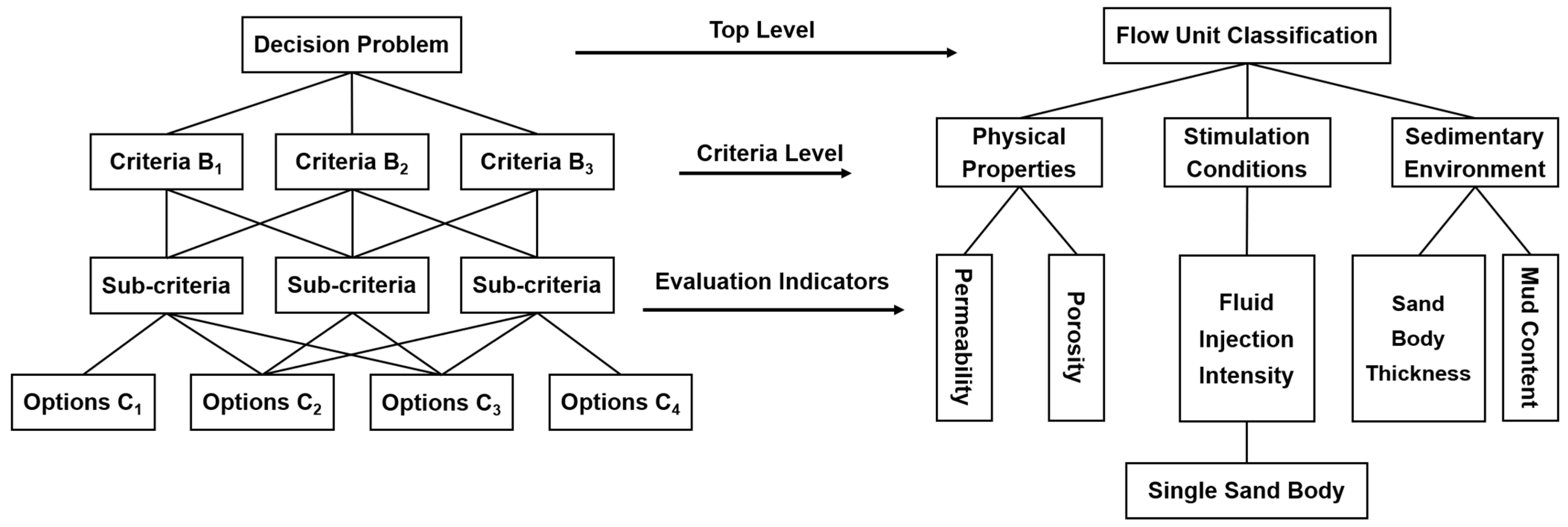
4.1. Subjective Weight Calculation Based on the AHM Method

The AHM method (Attribute Hierarchy Model) is an unstructured decision-making method that was proposed by Professor Cheng Gansheng in the 1990s [25]. It typically divides the hierarchy into three levels:

• Top level: contains only one element, representing the overall goal of the decision analysis, also known as the general objective level.
• Middle level: comprises several sub-objectives, representing the main goal and various sub-goals, often called the goal level.
• Bottom level: presents feasible methods to achieve each administrative decision objective, also known as the option level.

Based on these principles, a hierarchical model for dividing flow units in tight reservoirs in the study area was established (Figure 3). Here, the classification of tight reservoir flow units in Block W is the general objective, while sedimentary environment, physical properties, and stimulation conditions are the criteria levels for the target area. Each main criterion is further divided into sub-criteria as evaluation indicators: sedimentary environment includes effective sand body thickness and mud content, physical properties include porosity and permeability, and stimulation condition is represented by fluid injection intensity. These criteria and indicators form the hierarchical structure model for dividing tight reservoir flow units in Block W.

4.1.1. Constructing the Judgment Matrix

Based on the sample data, there are m objectives (criteria and sub-criteria). We compare these m indicators and note the relative importance of the i-th indicator to the j-th indicator as a_ij. This forms an m-order matrix to calculate the priority weights of each indicator for a certain standard, resulting in a weight analysis judgment matrix, also known as a judgment matrix, denoted as A = (a_ij)_n×n.

$$A={\left(a_{ij}\right)}_{n\times n}$$

(4)

In Equation (4), a_ij > 0, a_ij = 1/a_ji, a_ii =1, i, j = 1, 2, …, n.

Using the scale of relative importance between attributes proposed by Saaty, values for a_ij are calculated [26]. Specifically, in the Analytic Hierarchy Process (AHP), Saaty’s comparison scale is used to assess the relative importance of two criteria: 1 indicates equal importance; 3, 5, 7, and 9 represent increasing levels of importance from slight to extreme; while intermediate values of 2, 4, 6, and 8 are used for finer distinctions. The corresponding reciprocal values are applied to indicate reverse importance. Using the expert scoring method in petroleum field development geology, the five elements of the criteria level are analyzed and compared for importance according to Saaty’s comparison scale. This process produces the judgment matrix of the criteria level (physical properties, stimulation conditions, and sedimentary environment) for the target level in terms of tight reservoir flow units in Block W. Additionally, it produces the AHP judgment matrices for the indicator level against each criterion level: porosity and permeability for physical properties, fluid injection intensity for stimulation conditions, and effective sand body thickness and mud content for sedimentary environment, as shown in Equations (5) to (8):

• AHP Judgment Matrix of the Criteria Level

  $$A={\left(a_{ij}\right)}_{3\times 3}=\left[\begin{array}{ccc}1& 1/3& 3\\ 3& 1& 1/9\\ 1/3& 9& 1\end{array}\right]$$

  (5)
• AHP Judgment Matrix for Physical Properties

  $$B_1={\left(a_{ij}\right)}_{2\times 2}=\left[\begin{array}{cc}1& 5\\ 1/5& 1\end{array}\right]$$

  (6)
• AHP Judgment Matrix for Stimulation Conditions

  $$B_2={\left(a_{ij}\right)}_{1\times 1}=\left[1\right]$$

  (7)
• AHP Judgment Matrix for Sedimentary Environment

  $$B_3={\left(a_{ij}\right)}_{2\times 2}=\left[\begin{array}{cc}1& 3\\ 1/3& 1\end{array}\right]$$

  (8)

4.1.2. Constructing the Attribute Judgment Matrix

For each element in the top and middle levels, these are taken as the standard and an attribute judgment matrix is established with its corresponding lower-level elements. This calculates the attribute weights, or subjective weights.

In other words, attribute judgment matrices can be created for the three criteria levels: physical properties, stimulation conditions, and sedimentary environment. First, let B be a criterion, and let b₁, b₂, …, b_n be the indicators under this criterion. Compare the different indicators b_i and b_j (i ≠ j), and denote their relative importance to B as b_i and b_j, respectively. According to relevant requirements, u_ij and u_ji must satisfy the following:

$$\begin{array}{l}{u}_{ij}\ge 0,u_{ji}\ge 0,u_{ij}+u_{ji}=1,i\ne j;\\ u_{ij}=0,i=j,1\le i\le n,1\le j\le n\end{array}$$

(9)

The u_ij values that meet the above conditions are the relative attribute measures, and the matrix (u_ij) 1 ≤ i, j ≤ n formed is the attribute judgment matrix. The matrix (u_ij) 1 ≤ i, j ≤ n is generally obtained from the judgment matrix (a_ij) 1 ≤ i, j ≤ n using Equation (10), where k represents a positive integer no less than 1.

$$u_{ij}=\left\{\begin{array}{l}{\displaystyle \frac{k}{k+1}},a_{ij}=k,i\ne j\\ {\displaystyle \frac{1}{k+1}},a_{ij}={\displaystyle \frac{1}{k}},i\ne j\\ 0,a_{ij}=1,i=j\end{array}\right.$$

(10)

Equation (10) allows each level’s judgment matrix to be converted into the AHM attribute judgment matrix, with the results shown in Equations (11) to (14).

• AHM Attribute Judgment Matrix of the Criteria Level

  $$A^{*}={\left(u_{ij}\right)}_{3\times 3}=\left[\begin{array}{ccc}0& 1/4& 3/4\\ 3/4& 0& 1/10\\ 1/4& 9/10& 0\end{array}\right]$$

  (11)
• AHM Attribute Judgment Matrix for Physical Properties

  $${B_1}^{*}={\left(u_{ij}\right)}_{2\times 2}=\left[\begin{array}{cc}0& 5/6\\ 1/6& 0\end{array}\right]$$

  (12)
• AHM Attribute Judgment Matrix for Stimulation Conditions

  $${B_2}^{*}={\left(u_{ij}\right)}_{1\times 1}=\left[0\right]$$

  (13)
• AHM Attribute Judgment Matrix for Sedimentary Environment

  $${B_3}^{*}={\left(u_{ij}\right)}_{2\times 2}=\left[\begin{array}{cc}0& 3/4\\ 1/4& 0\end{array}\right]$$

  (14)

The relative weight of the criteria level (physical properties, sedimentary environment, and stimulation conditions) is defined, with respect to the decision level, as W_b. The relative weights of the indicator level, with respect to the previous level, are defined as W_c1, W_c2, W_c3.

4.1.3. Attribute Weight Calculation

There is consistency within the attribute judgment matrix (u_ij) _1≤i,j≤n, so it is not necessary to estimate the eigenvalues and eigenvectors of the matrix, nor is consistency verification required. The formula for calculating the weight W_b is

$$W_b={\left[W_b(1),W_b(2),\dots ,W_b(n)\right]}^T={\displaystyle \frac{2}{n(n-1)}}{\displaystyle \sum _{j=1}^n{u}_{ij}},1\le i\le n$$

(15)

where W_b(n) represents the relative weight of the n-th indicator.

From the attribute judgment matrix in Equation (11), the relative weights of the three criteria levels—physical properties B₁, stimulation conditions B₂, and sedimentary environment B₃—with respect to the decision level (the division of tight reservoir flow units in Block W A), are W_b = [1/3,17/60,23/60]^T.

From the attribute judgment matrix in Equation (12), the relative weights of the indicator level—permeability C₁ and porosity C₂—with respect to the criteria level physical properties B₁ are W_c1 = [5/6,1/6]^T.

From the attribute judgment matrix in Equation (14), the relative weights of the indicator level—sand body thickness C₄ and mud content C₅—with respect to the criteria level sedimentary environment B₃ are W_c3 = [3/4,1/4]^T.

4.1.4. Calculation of Combined Weights

We calculate the ranking weights of each major factor in a level relative to the top level, which provides the combined weight of each indicator. This step is performed progressively from top to bottom. We assume the previous level A contains m indicators A₁, A₂, …, A_n with weights a₁, a₂, …, a_n; the next level B contains n elements B₁, B₂, …, B_n. The weights for each factor B_j in the single-criterion ranking are b_1j, b_2j…, b_nj (where b_kj = 0 if B_k is unrelated to A_k). The combined weights for level B can then be calculated using Equation (16).

$$b_k={\displaystyle \sum _{j=1}^m{a}_j{b}_{kj}}$$

(16)

Using the combined weight formula W_c = W_b × W_c(n), we calculate the combined weights of each indicator level relative to the target level as W_c = [5/18,1/18,17/60,23/80,23/240]^T. Converted to decimal form, this gives W_c = [0.278,0.056,0.283,0.2875,0.0958]^T.

4.2. Objective Weight Calculation Based on Entropy Weight Method

Entropy is an index reflecting the degree of uncertainty in an information system; the higher the entropy value, the more dispersed the data layout, indicating stronger uncertainty. In weight classification, the more dispersed the distribution of the j-th indicator, the greater its importance in the corresponding index [27,28,29,30,31].

4.2.1. Constructing the Initial Indicator Matrix

Based on the basic data, we construct the initial indicator matrix as follows:

$$X=\left[\begin{array}{ccc}{x}_{11}& \cdots & x_{1n}\\ ⋮& ⋮& ⋮\\ x_{m1}& \cdots & x_{mn}\end{array}\right]$$

(17)

where m is the number of samples, n is the number of indicators, and x_ij is the value of the j-th indicator for the i-th sample.

From X, we can see that each sample has five characteristic indicators, but it is not certain in advance which indicator holds the advantage. In other words, X represents a certain level of uncertainty, and entropy is the measure of this uncertainty.

4.2.2. Matrix Normalization

Since all indices have different dimensions and large data variations, it is necessary to standardize (dimensionless) each index to ensure consistency.

$$z_{ij}={\displaystyle \frac{x_{ij}}{{\displaystyle \sum _{i=1}^m{x}_{ij}}}}$$

(18)

The normalized matrix can be obtained based on Equation (18):

$$Z=\left[\begin{array}{ccc}{z}_{11}& \cdots & z_{1n}\\ ⋮& ⋮& ⋮\\ z_{m1}& \cdots & z_{mn}\end{array}\right]$$

(19)

For the tight reservoir in Block W, the initial matrix was normalized to obtain the processed standardized matrix.

4.2.3. Calculating Information Entropy

The formula for calculating information entropy is as follows:

$$e_j=-{\displaystyle \sum _{i=1}^m{z}_{ij}\ln }{z}_{ij}$$

(20)

Using Equation (20), the information entropy values for each target parameter are calculated as follows:

$$e_j={\left[3.31513.39503.34873.34733.3801\right]}^T$$

(21)

4.2.4. Calculating Indicator Divergence

The formula for calculating indicator divergence h_j is as follows:

$$h_j=1-{\displaystyle \frac{e_j}{\ln m}}$$

(22)

Here, if the values of the j-th indicator are more widely distributed, the corresponding h_j value will be larger, indicating a higher importance of the j-th indicator.

Using Equation (22), the indicator divergence for each target parameter is calculated as follows:

$$h_j={\left[0.02530.00180.01540.01580.0062\right]}^T$$

(23)

4.2.5. Calculating Indicator Weights

Among the n included indicators, the weight of the j-th indicator is as follows:

$$w_j={\displaystyle \frac{h_j}{{\displaystyle \sum _{j=1}^n{h}_j}}}$$

(24)

Using Equation (24), the indicator weights for each target parameter are calculated as follows:

$$w_j={\left[0.39180.02810.23880.24510.0963\right]}^T$$

(25)

4.3. Comprehensive Weight Calculation Based on the Entropy Weight–AHM Method

Using either the entropy weight method or the AHM method alone to calculate weights only considers subjective or objective factors, which does not fully capture the characteristics of flow units in the target tight reservoir. Therefore, a combined approach incorporating both the entropy weight and AHM methods is proposed, introducing a comprehensive weight $W=\left[W^{\prime },W^{″}\right]$. Here, $W^{\prime }$ represents the subjective weight and $W^{″}$ represents the objective weight, combining both subjective and objective factors to calculate the weights [32,33,34,35,36].

For the entropy weight–AHM method, assume there are m core samples and n parameters for flow unit division, forming an original data matrix [x_ij]_m×n. Using the range transformation method (Equation (18)) for normalization, we obtain a normalized matrix [z_ij]_m×n. Let z_j^max represent the maximum value in the j-th column of [z_ij]_m×n; then, the point {z₁^max z₂^max, …, z_n^max} forms the ideal point in the sample space. Let α and β represent the importance of subjective and objective weights $W^{\prime }$ and $W^{″}$, and establish the following optimization model:

$$\max (L)={\displaystyle \sum _{j=1}^n\left(\alpha W^{\prime }+\beta W^{″}\right)}{\left(z_j^{\max }-z_{ij}\right)}^2$$

(26)

Let ${\alpha }^2+{\beta }^2=1$, and set ${\alpha }^{\ast }={\displaystyle \frac{\alpha }{\alpha +\beta }}$, ${\beta }^{\ast }={\displaystyle \frac{\beta }{\alpha +\beta }}$. Further calculations on this optimization model yield the final comprehensive weights:

$$W={\alpha }^{\ast }{W}^{\prime }+{\beta }^{\ast }{W}^{″}$$

(27)

where ${\alpha }^{\ast }={\displaystyle \frac{{\displaystyle \sum _{j=1}^n{W_j}^{\prime }}{\left(z_j^{\max }-z_{ij}\right)}^2}{{\displaystyle \sum _{j=1}^n\left({W_j}^{\prime }+{W_j}^{″}\right)}{\left(z_j^{\max }-z_{ij}\right)}^2}}$, ${\beta }^{\ast }={\displaystyle \frac{{\displaystyle \sum _{j=1}^n{W_j}^{″}}{\left(z_j^{\max }-z_{ij}\right)}^2}{{\displaystyle \sum _{j=1}^n\left({W_j}^{\prime }+{W_j}^{″}\right)}{\left(z_j^{\max }-z_{ij}\right)}^2}}$.

Using the normalized matrix obtained through the range transformation method, calculations based on Equations (26) and (27) yield $\alpha *=0.5137,\beta *=0.4863$. Further calculations produce the comprehensive weight values for each evaluation indicator:

$$W={\left[0.33330.04240.26150.26690.0960\right]}^T$$

(28)

From the comprehensive weight values, it can be seen that in the process of dividing flow units in the target tight reservoir, the relative importance of the five selected evaluation indicators is as follows: permeability > sand body thickness > fluid injection intensity > mud content > porosity.

The classification standards for reservoir flow units were derived from the normal distribution pattern of the samples’ indicator comprehensive scores (

Table 1. Evaluation standard of reservoir flow unit based on entropy weight–AHM method.

Indicator Comprehensive Score	Type
>0.54	Fu1
0.48~0.54	Fu2
0.38~0.48	Fu3
<0.38	Fu4

).

Based on the reservoir flow unit evaluation standards from the entropy weight–AHM method (Table 1), and combining the weighted calculation results of each flow unit, the reservoir flow unit evaluation results are obtained (

Table 2. Division results of reservoir flow units based on entropy weight–AHM method.

Flow Units	Sand Body Thickness (m)	Permeability (10−3 μm2)	Mud Content (%)	Porosity (%)	Fluid Injection Intensity (m3/m)	Comprehensive	Type
S1-1	3.28	0.23	19.17	11.18	33.80	0.30	Fu4
S1-2	4.58	0.21	25.71	11.03	38.95	0.33	Fu4
S1-3	6.76	0.28	19.40	11.14	25.40	0.37	Fu4
S2-1	6.88	0.12	17.28	9.27	48.63	0.46	Fu3
S2-2	5.89	0.59	22.91	12.67	30.53	0.51	Fu2
S3-1	6.4	0.45	22.45	11.17	26.80	0.43	Fu3
S3-2	4.1	0.26	22.22	10.31	26.80	0.26	Fu4
S3-3	4.31	0.75	21.54	12.83	20.65	0.48	Fu2
S4-1	4.69	0.61	20.54	11.95	33.74	0.52	Fu2
…	…	…	…	…	…	…	…
S7-1	6.78	0.44	23.02	11.59	12.27	0.33	Fu4
S7-2	5.39	0.43	13.34	11.70	12.27	0.34	Fu4
S8-1	6.23	0.81	21.77	13.11	30.88	0.64	Fu1
S8-2	4.75	0.75	20.53	12.12	38.55	0.62	Fu1
S8-3	10.89	0.31	16.46	10.44	38.85	0.62	Fu1
S9-1	5.59	0.21	10.72	10.69	40.87	0.46	Fu3
S9-2	5.59	0.53	25.99	12.45	31.60	0.46	Fu3
S9-3	9.85	0.63	16.78	13.25	13.70	0.57	Fu1
S10-1	4.23	0.48	12.69	12.93	24.88	0.44	Fu3
S10-2	6	0.46	19.96	11.73	40.23	0.53	Fu2
S10-3	3.94	0.71	16.15	14.17	23.75	0.51	Fu2

).

4.4. Reliability Demonstration

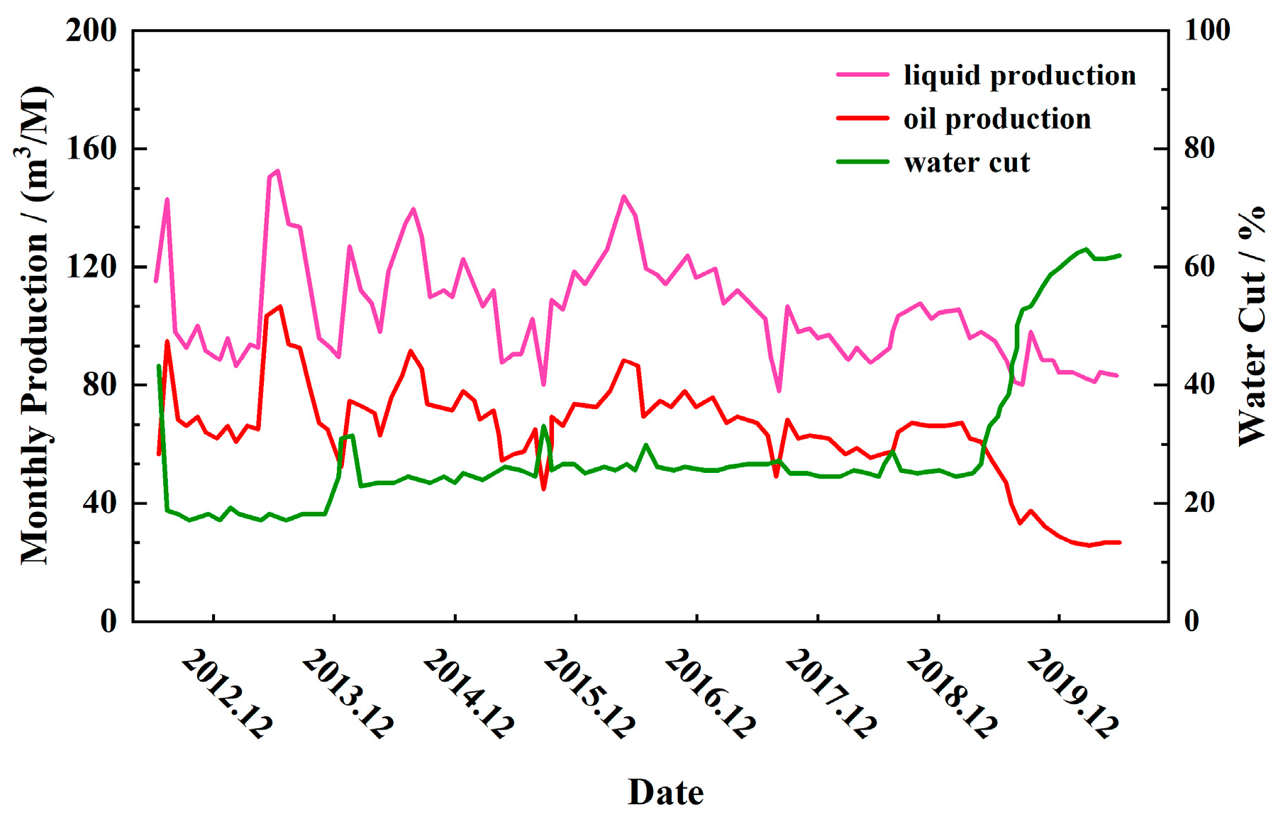
4.4.1. Testing with Production Dynamics Parameters

Reference [37] indicates that the frequency of intercalations has a significant impact on the production of oil wells. Wells with underdeveloped sand bodies typically have lower production and experience a faster decline in output, while wells with well-developed sand bodies show higher production and more stable production changes. Based on the above principles, using the entropy weight–AHM method, reservoir flow units in the study area were characterized, and a well-to-well flow unit profile was created for wells P68-P71 (Figure 4). First, spatial variogram functions are constructed using well point data to quantify the spatial correlation between well points. Then, combining logging data, well point data, and geological background information, Kriging interpolation is applied to predict the spatial distribution and distribution pattern of flow units. Finally, the entropy-weighted–AHM method is used to classify the reservoir flow units in the study area. Based on the classification results, the flow unit connection profiles of wells P68 to P71 are prepared to display the spatial distribution and connectivity characteristics of each flow unit.

Figure 4 shows that production well P69 has well-developed sand bodies, mostly classified as Fu₁, with a large thickness and few interlayers. In the Figure 4, the blue arrows indicate injection wells, and the red arrows indicate production wells. Figure 5 proves that well P69 should have relatively high production (around 70 t/M). In contrast, production well P71 has less-developed sand bodies, poorer reservoir properties, and only a small portion of Fu₁ flow units. Figure 6 proves that well P71 should have a relatively low production capacity (around 10 t/M).Therefore, from the perspective of reservoir development and production dynamics, characterizing reservoir flow units based on the entropy weight–AHM method is reliable.

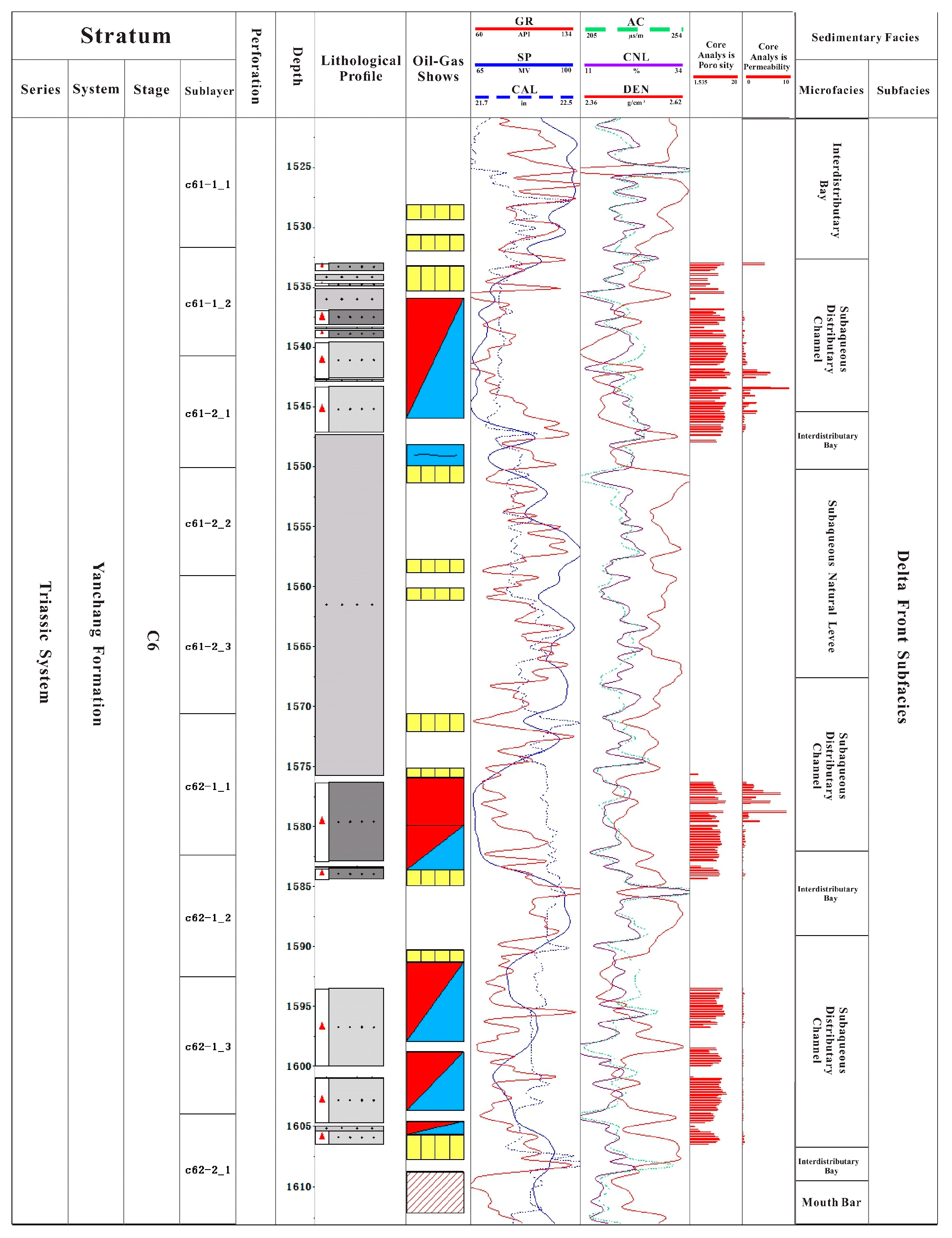
4.4.2. Testing the Distribution of Flow Units

Reference [38] uses the flow unit characterization results to create a lateral distribution map of flow units at the sublayer level, in order to verify the reliability of the flow unit characterization results. Based on the characterization results of single-well reservoir flow units, Petrel was used to model the reservoir flow units. Figure 7a shows the flow unit distribution map for the non-main layers, while Figure 7b shows the flow unit distribution for the main layers (Figure 7). Comparing the distribution maps of the main and non-main layers shows that the non-main layers are primarily composed of Fu₃ and Fu₄ flow units, while the main layers are dominated by Fu₁ and Fu₂ flow units. Therefore, from the perspective of flow unit distribution, the flow units divided based on the entropy weight–AHM method are reliable.

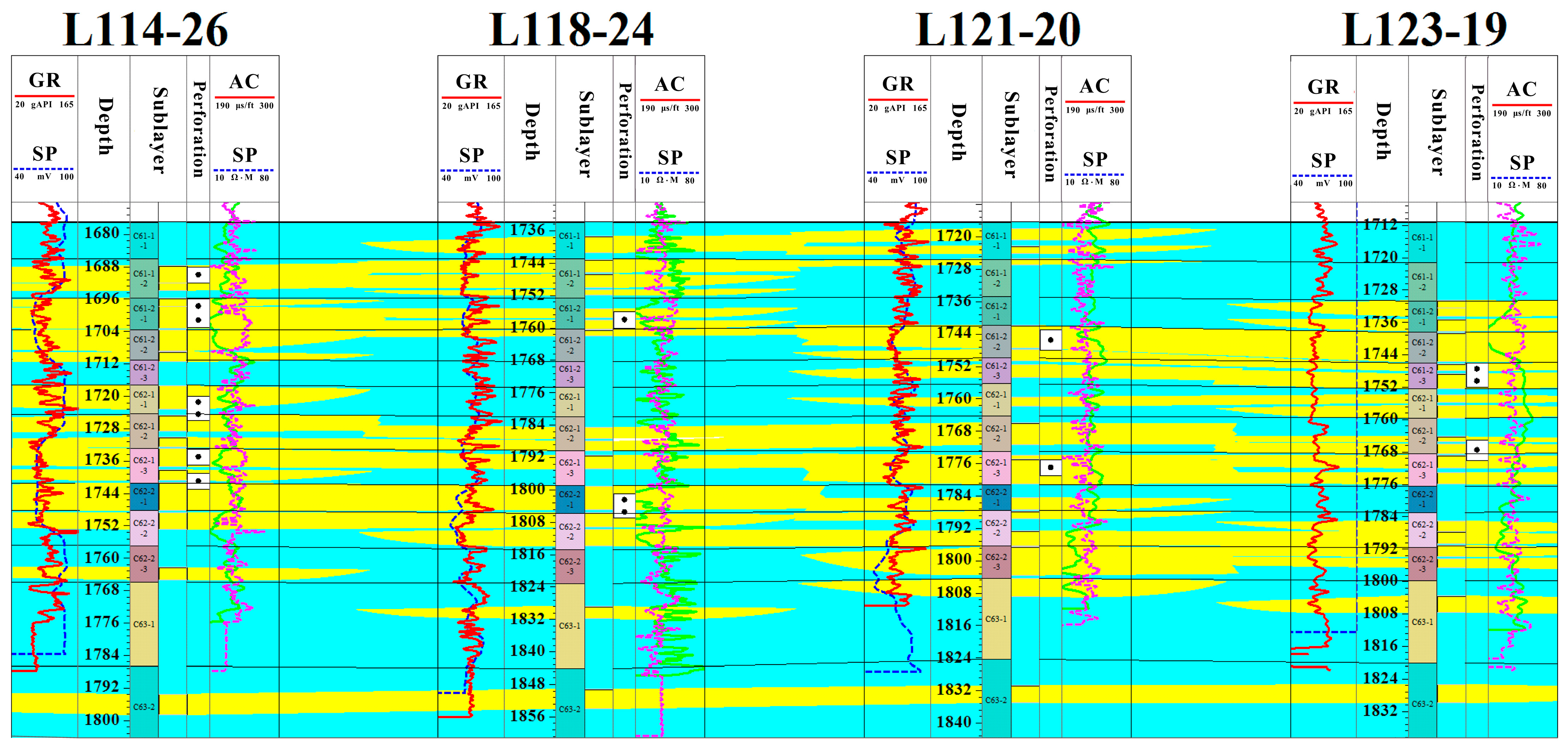
4.4.3. Testing Flow Unit Comparison

A comparison of logging parameters was conducted across different types of flow units, and the attribute parameters for the four types of flow units calculated for the entire area show that (

Table 3. Statistical table of flow unit division result parameters in target area.

Flow Unit	Sand Body Thickness (m)	Permeability (10−3 μm2)	Porosity	Mud Content (%)
Fu1	14.1	4.24	0.14	11.5
Fu2	7.2	2.45	0.11	13.4
Fu3	2.4	3.24	0.13	15.7
Fu4	2.1	0.86	0.08	21.3

), in terms of classification, Fu₁ has better physical properties than Fu₂, Fu₂ is superior to Fu₃, and Fu₄ has the poorest physical properties. Reference [39] also obtained the same results, dividing the flow units into six categories, with significant physical property differences between them. Therefore, from the perspective of differences in flow unit types, the flow units divided based on the entropy weight–AHM method and human–machine interaction are reliable.

The flow unit characterization results of this method have been validated in the Block W reservoir, but its application in other complex reservoirs still needs further evaluation and verification.

In practical production, the boundaries and distribution patterns of reservoir flow units may change with variations in the formation shape. Therefore, it is possible to adjust the flow unit characterization results by combining actual production data and formation pressure data to better utilize the dynamic characteristics of the reservoir.

The flow unit characterization results can be integrated with the reservoir numerical simulation model, which allows for a more comprehensive consideration of the reservoir’s complexity, enabling more accurate predictions of production dynamics and providing a more reliable basis for the optimization of development plans.

5. Application

5.1. Analysis of Stimulation Measure Compatibility

Many scholars adjust the enhanced recovery measures based on the flow unit characterization results [40,41,42]. In this study, based on the flow unit characterization results from the entropy weight–AHM method, a grid map of flow units in Block W was created to analyze reservoir geological features in 3D space. Existing measures and production dynamics data were then used to assess the compatibility of measures with production wells, establishing a compatibility evaluation standard. The premise of the compatibility analysis is that the perforation locations of the production wells must intersect with developed sand bodies. Conversely, if the perforation locations do not intersect with developed sand bodies, no compatibility analysis for enhanced recovery measures will be performed.

5.1.1. Poor Compatibility

Poor compatibility means mismatches in perforation positions between injection and production wells and insufficient stimulation for the production well. In Figure 8, the first perforation section of well P62 has developed sand bodies, but the injection well P61 does not, so P62 and P61 cannot form an effective injection–production relationship in this section. In the second perforation section, both P62 and P61 have developed sand bodies. However, the flow unit analysis shows that P61 is a Fu₂ flow unit with better reservoir properties, while P62 is a Fu₃ flow unit with poorer properties. Since P62 has lower reservoir quality, it needs a stronger stimulation to improve. But the analysis shows that P62’s stimulation intensity is low, indicating poor connectivity between the wells in the second perforation section.

Stimulation measures that fail to establish a good injection–production relationship or have poor sand body connectivity are classified as poorly compatible with the tight reservoirs in the study area.

5.1.2. Moderate Compatibility

Moderate compatibility means there is either a mismatch in perforation positions between injection and production wells or an inadequate stimulation intensity. As shown in Figure 9, in the first perforation section of well P82, the stimulation intensity is insufficient, resulting in a Fu₃ flow unit. The corresponding injection well P81, is a Fu₁ flow unit, but there is still no good sand body connectivity between the injection and production wells.

Stimulation measures that result in poor sand body connectivity or have mismatches between perforation positions and sand body locations are classified as moderately compatible with the tight reservoirs in the target area.

5.1.3. Good Compatibility

Good compatibility means that perforation positions between injection and production wells are matched, and the stimulation intensity is appropriate. As shown in Figure 10, after fracturing in the first perforation section of well P86, both the production and injection wells are Fu₁ flow units, indicating a good connectivity between them.

Stimulation measures that create good sand body connectivity and align perforation positions with sand body locations are classified as well matched to the tight reservoirs in the target area.

5.2. Differential Adjustment Strategies for the Target Area

Based on the compatibility of the sand body properties with the stimulation treatments, recommendations for different well sections in the tight reservoir study area are provided.

Table 4. Differentiated adjustment table under the compatibility of different measures.

Treatments Compatibility	Evaluation Standard	Adjustment Strategy
Poor	Perforation positions do not match; stimulation intensity is inadequate	Adjust perforation positions and increase stimulation intensity
Moderate	Perforation positions or stimulation intensity do not match	Increase stimulation intensity and adjust perforation positions
Good	Perforation positions and stimulation intensity both match	No adjustment; use parameters as a referencefor other wells

summarizes the compatibility levels and the corresponding adjustment strategies. As shown in Table 4, for poor- or moderate-compatibility measures, improvements include adjusting the perforation positions and increasing the stimulation intensity. For good compatibility, where both perforation positions and stimulation intensity are compatible, these parameters can be used as a reference to guide the stimulation treatments for other wells.

This method has been successful in guiding the application of artificial stimulation treatments, but there are still the following shortcomings:

• The method relies on static geological parameters and dynamic artificial stimulation intensity parameters. However, in practical applications, difficulties in data acquisition and high data noise may arise, affecting the accuracy and reliability of the model.
• During long-term reservoir production, fracture systems may become blocked or closed, affecting the distribution of flow units. However, the model has limitations in dynamically reflecting fracture changes.
• The model uses the entropy-weighting method to assign weights to static and dynamic parameters, simplifying the complex interactions between them, which may introduce errors.

6. Conclusions

This study focuses on the tight reservoir in Block W, using the Grey Relational Analysis method to identify key parameters that influence the properties of flow units in tight reservoirs. The entropy weight–AHM method was then developed and applied to study the flow units in the study area. The main conclusions are as follows:

(1)

By integrating the seepage mechanism of tight oil reservoirs and field practices, the Grey Relational Analysis method was used to select the key static parameters (sand body thickness, permeability, mud content, and porosity) and stimulation parameter (fluid injection intensity) that affect the properties of flow units in tight reservoirs.

(2)

This study establishes the entropy weight–AHM method, which incorporates both subjective and objective weights to achieve comprehensive flow unit characterization in tight reservoirs. This method calculated the comprehensive weights and scores for flow unit indicators in Block W, enabling the interactive characterization of flow units in tight reservoirs. Flow unit classification standards were provided based on normal distribution, and the method’s reliability was verified through production dynamics and other factors.

(3)

Based on the flow unit characterization results for Block W, key flow unit maps were created. Combined with existing stimulation treatments and production dynamics data, these maps were used to evaluate the compatibility of measures with production wells. A compatibility evaluation standard was established, guiding the next steps in development adjustments for Block W.

References

1. Gunter, G.W.; Finneran, J.M.; Hartmann, D.J.; Miller, J.D. Early determination of reservoir flow units using an integrated petrophysical method. In Proceedings of the SPE Annual Technical Conference and Exhibition, San Antonio, TX, USA, 5–8 October 1997. [Google Scholar]
2. Aguilera, R. Flow units: From conventional to tight-gas to shale-gas to tight-oil to shale-oil reservoirs. SPE Reserv. Eval. Eng. 2014, 17, 190–208. [Google Scholar] [CrossRef]
3. Rodriguez, A. Facies modeling and the flow unit concept as a sedimentological tool in reservoir description: A case study. In Proceedings of the SPE Annual Technical Conference and Exhibition, Houston, TX, USA, 2–5 October 1988. [Google Scholar]
4. Nooruddin, H.A.; Hossain, M.E. Modified kozeny–carmen correlation for enhanced hydraulic flow unit characterization. J. Pet. Sci. Eng. 2011, 80, 107–115. [Google Scholar] [CrossRef]
5. Kassab, M.A.; Teama, M.A. Hydraulic flow unit and facies analysis integrated study for reservoir characterisation: A case study of Middle Jurassic rocks at Khashm EI-Galala, Gulf of Suez, Egypt. Arab. J. Geosci. 2018, 11, 294. [Google Scholar] [CrossRef]
6. Wang, H.; Kou, Z.; Bagdonas, D.A.; Phillips, E.H.; Alvarado, V.; Johnson, A.C.; Jiao, Z.; McLaughlin, J.F.; Quillinan, S.A. Multiscale petrophysical characterization and flow unit classification of the minnelusa eolian sandstones. J. Hydrol. 2022, 607, 127466. [Google Scholar] [CrossRef]
7. Amaefule, J.O.; Altunbay, M.; Keelan, D.K. Enhanced Reservoir Description: Using Core and Log Data to Identify Hydraulic (Flow) Units and Predict Permeability in Uncored Intervals/Wells. In Proceedings of the SPE Annual Technical Conference and Exhibition, Houston, TX, USA, 3–6 October 1993. [Google Scholar]
8. Silseth, J.K.; MacDonald, A.C.; Alvestad, J.; Buller, A.T.; Torp, S.B. Impact of Flow-Unit Reservoir Description on Simulated Waterflood Performance. SPE Reserv. Eng. 1993, 8, 27–33. [Google Scholar] [CrossRef]
9. Ti, G.; Ogbe, D.O.; Munly, W.; Hatzignatiou, D.G. Use of Flow Units as a Tool for Reservoir Description: A Case Study. SPE Form. Eval. 1995, 10, 122–128. [Google Scholar] [CrossRef]
10. Li, H.; Peng, S. Reservoir dynamic flow unit models of Jing11 block in Bieguzhuang oilfield. Pet. Geol. Recovery Effic. 2007, 149, 67–70. [Google Scholar]
11. Song, G.; Sun, W.; Gao, H.; Mo, J. The classification of flow units and its influence on deliverability performance: A case of the Chang 1 formation of Yuan 54 Areas in Ordos Basin. J. Northwest Univ. (Nat. Sci. Ed.) 2010, 40, 299–303. [Google Scholar]
12. Xu, S.; Lu, Y.; Wang, Y. Study on Flow Units of Turbidite Fan Low Permeability Reservoir Based on Support Vector Machine. J. Jilin Univ. (Earth Sci. Ed.) 2018, 48, 1330–1341. [Google Scholar]
13. Yu, P. An integrated method of data mining and flow unit identification for typical low permeability reservoir prediction. World J. Eng. Technol. 2018, 7, 122–128. [Google Scholar] [CrossRef]
14. Lu, Y.; Liu, K.; Xu, S.; Wang, Y.; Zhang, Q. Identifying flow units by FA-assisted SSOM—An example from the eocene basin-floor-fan turbidite reservoirs in the daluhu oilfield, dongying depression, bohai bay basin, china. J. Pet. Sci. Eng. 2020, 186, 106695. [Google Scholar] [CrossRef]
15. Yuan, B.; Zhang, H.; Ye, Q.; Zhang, L.; Chen, Z.; Yao, C.; Dong, D.; Lai, J. Flow-unit Classification Based on Compound Sand-Body Architecture of Delta and Distribution Pattern of Remaining Oil. Acta Sedimentol. Sin. 2021, 39, 1253–1263. [Google Scholar]
16. Liu, R.; Sun, Y.; Yan, B. Reservoir Flow Units for Dynamic and Static Combinations: Case study of Neogene Guantao Formation in block M, Gudao oilfield. Acta Sedimentol. Sin. 2023, 41, 1170–1180. [Google Scholar]
17. Ding, Y.; Guo, X.; Chang, S. Research on identification of flow units based on FZI. EDP Sci. 2021, 248, 01005. [Google Scholar]
18. Farzi, R.; Bolandi, V.; Yarmohammadi, S.; Mosalmannejad, H.; Ezati, M. Intelligent and Statistical Analysis to Estimating the Hydraulic Flow Units: A Case Study from the Kupal Oilfield, SW Iran. J. Appl. Geophys. 2022, 206, 104814. [Google Scholar] [CrossRef]
19. Zhang, J.; Yan, D.; Zhou, S.; Wang, H.; Deng, Y.; Liu, E.; Song, G. Sedimentological and Diagenetic Effects on Petrophysical Characteristics and Hydraulic Flow Units of Zhujiang Sandstones in the Pearl River Mouth Basin, South China Sea. Energy 2023, 282, 128942. [Google Scholar] [CrossRef]
20. Foroshani, J.S.; Mehrabi, H.; Rahimpour-Bonab, H. Reservoir Heterogeneity of Upper Cretaceous Sarvak Formation in the Dezful Embayment, SW Iran: Implications of Flow Unit Distribution, Electrofacies Analysis and Geological-Based Reservoir Zonation. J. Afr. Earth. Sci. 2023, 200, 104882. [Google Scholar] [CrossRef]
21. Cabrera Ruiz, M.L.; Batezelli, A. Correlation between Geomechanical and Sedimentary Facies and Their Implications for Flow Unit Definition in the Pre-Salt Carbonate Reservoir, Brazil. J. South Am. Earth Sci. 2024, 141, 104958. [Google Scholar] [CrossRef]
22. Xu, Z.; Fu, Q.; Hui, X.; Jing, L.; Shixiang, J.; Xiangtong, L. Division and distribution of flow units of Chang 613reservoir in Huaqing area, Ordos Basin. Nat. Gas Geosci. 2018, 29, 1757–1766. [Google Scholar]
23. Yan, W.; Bao, H.; Si, X.; Yu, Y. Optimization of fracturing parameters for horizontal wells based on grey correlation method. Math. Pract. Theory 2021, 51, 145–151. [Google Scholar]
24. Yang, J.; Jiang, Z. Application of Grey Relational Analysis in Urumqi Mining Area Reservoir Assessment. Coal Geol. China 2017, 29, 36–40. [Google Scholar]
25. Dong, F.; Lu, X.; Jin, W. The Comprehensive Evaluation of Low Permeability Sandstone Reservoirs Based on the AHM Method. Ground Water 2016, 38, 168–170. [Google Scholar]
26. Harker, P.T.; Vargas, L.G. The theory of ratio scale estimation: Saaty’ analytic hierarchy process. Manag. Sci. 1987, 33, 1383–1403. [Google Scholar] [CrossRef]
27. Dong, F.; Lu, X.; Ju, H.; Wei, S. Division of Flow Units of the Low Permeability Sandstone Reservoir Based on Entropy-Weighting TOPSIS Method. Bull. Geol. Sci. Technol. 2012, 31, 124–128. [Google Scholar]
28. Zhang, T.; Yan, H. Optimization and Application of Multi-attribute Decision Algorithm Based on Entropy Weight Method. J. North China Univ. Sci. Technol. (Nat. Sci. Ed.) 2022, 44, 82–88. [Google Scholar]
29. Li, F.; Li, D. Combination Evaluation Model Based on the Entropy Weight Method. Technol. Informatiz. 2021, 148–150. [Google Scholar]
30. Yang, W.; Wu, Y.; Wang, J. Grey Confidence Interval Estimation of Small Samples Based on Entropy-weight Method. J. Zhengzhou Univ. (Nat. Sci. Ed.) 2016, 48, 51–56. [Google Scholar]
31. Zhou, R.; Fan, F.; He, D.; Qiu, W.H. Integrated entropy weight method based on data stability and subjective preference in multi-attribute group decision-making. Control Decis. 2012, 27, 1169–1174. [Google Scholar]
32. Cao, C.; Zhou, F.; Cheng, L.; Liu, S.; Lu, W.; Wang, Q. A comprehensive method for acid diversion performance evaluation in strongly heterogeneous carbonate reservoirs stimulation using CT. J. Pet. Sci. Eng. 2021, 203, 108614. [Google Scholar] [CrossRef]
33. Xue, Y.; Cheng, L.; Mou, J.; Zhao, W. A new fracture prediction method by combining genetic algorithm with neural network in low-permeability reservoirs. J. Pet. Sci. Eng. 2014, 121, 159–166. [Google Scholar] [CrossRef]
34. Cao, C.; Cheng, L.; Zhang, X.; Shi, J. Numerical simulation investigation on well performance integrated stress sensitivity and sand production. Geofluids 2021, 2021, 9925866. [Google Scholar] [CrossRef]
35. Liu, X.; Shen, N.; Feng, H. Application of the AHM Model Based on Entropy Weight in the Selection of Third-Party Logistics Carriers. China-Today Forum 2013, 56–57. [Google Scholar]
36. Dong, F.; Lu, X.; Chen, X.; Xin, T. Optimum Program for Underground Gas Storage Projects Based on Entropy-weight AHM. J. Yangtze Univ. (Nat. Sci. Ed.) 2012, 9, 133–136. [Google Scholar]
37. Zhang, L.; Li, R.; Deng, H.; Fu, M.; Hu, L.; Guo, X.; Xie, X.; Zhao, C. Identification, Distribution Characteristics, and Effects on Production of Interlayers in Carbonate Reservoirs: A Case Study from the Cretaceous Mishrif Formation in Halfaya Oilfield. Iraq. J. Pet. Sci. Eng. 2021, 202, 108571. [Google Scholar] [CrossRef]
38. Chen, H. Flow Unit Characteristics of Fan Delta Front Deposits and Its Influence on Reservoir Development-Taking Yulou Oil Bearing Sets in Some Experimental Area in West Depression in Liaohe Basin in China as an Example. J. Pet. Sci. Eng. 2019, 179, 44–55. [Google Scholar] [CrossRef]
39. Fan, Z.; Li, K.; Li, J.; Song, H.; He, L.; Wu, X. A Study on Remaining Oil Distribution in a Carbonate Oil Reservoir Based on Reservoir Flow Units. Pet. Explor. Dev. 2014, 41, 634–641. [Google Scholar] [CrossRef]
40. Chen, X.; Xiao, P.; Duan, R.; Lu, W.; Zhang, X.; Chen, G. Study on flow unit division and remaining oil tapping in deep-water turbidite gas injection reservoir. Unconv. Oil Gas 2023, 10, 103–111. [Google Scholar]
41. Chu, F.; Zhang, X.; Zhang, G.; Dong, C. Deep Learning Prediction of Waterflooding-Based Alteration of Reservoir Hydraulic Flow Unit. Geoenergy Sci. Eng. 2023, 231, 212396. [Google Scholar] [CrossRef]
42. Oliveira, G.P.; Araújo, E.A.; Santos, M.D.; Roque, W.L. Non-Uniform Injector/Producer Well Pattern Designs Induced by Morphology and Anisotropy of Flow Units. J. Pet. Sci. Eng. 2020, 186, 106680. [Google Scholar] [CrossRef]
Figure 1. Multi-well logging correlation profile.
Processes 12 02706 g001
Figure 2. Single-well columnar comprehensive analysis chart.
Processes 12 02706 g002
Figure 3. Hierarchical structure model of tight reservoir in Block W.
Processes 12 02706 g003
Figure 4. Well connection profile of flow unit of well P68–P71.
Processes 12 02706 g004
Figure 5. Development performance curve of well P69.
Processes 12 02706 g005
Figure 6. Development performance curve of well P71.
Processes 12 02706 g006
Figure 7. Plan of each sublayer flow unit. (a) Layer 1 flow unit distribution map. (b) Layer 7 flow unit distribution map.
Processes 12 02706 g007
Figure 8. Flow unit of well group P61 (partly).
Processes 12 02706 g008
Figure 9. Flow unit of well group P81 (partly).
Processes 12 02706 g009
Figure 10. Flow unit of well group P85 (partly).
Processes 12 02706 g010