Probabilistic Time Series Forecasting Based on Similar Segment Importance in the Process Industry

Abstract

Probabilistic time series forecasting is crucial in various fields, including reducing stockout risks in retail, balancing road network loads, and optimizing power distribution systems. Building forecasting models for large-scale time series is challenging due to distribution differences, amplitude fluctuations, and complex patterns across various series. To address these challenges, a probabilistic forecasting method with two different implementations that focus on historical segment importance is proposed in this paper. First, a patch squeeze and excitation (PSE) module is designed to preprocess historical data, capture segment importance, and distill information. Next, an LSTM-based network is used to generate maximum likelihood estimations of distribution parameters or different quantiles for multi-step forecasting. Experimental results demonstrate that the proposed PSE module significantly enhances the base model’s prediction performance, and direct multi-step forecasting offers more detailed information for high-frequency data than recursive forecasting.

1. Introduction

As automation and information technology advance, process industries—including chemical, pharmaceutical, light industry, metallurgy, and power generation—produce tens of thousands of sequential data points each day. Extracting valuable information from these complex time-series data is essential for maintaining safety, efficiency, and flexibility in production processes [1]. Additionally, process industries are connected to various sectors, either directly or indirectly, through energy and supply chains, including power generation, sales, and logistics [2]. Monitoring time series in related industries generates valuable feedback for process industries. For instance, forecasting power loads aids in adjusting energy consumption, while evaluating product demand helps guide production.

In other words, time series forecasting holds substantial value across many industries and serves as a key input for decision-making in various business actions [3]. For example, sales forecasting aids inventory management and resource scheduling [4,5], while power load and generation efficiency forecasting are crucial for optimizing transmission and distribution operations [6,7]. Traffic flow forecasting assists in road planning and network balancing [8], while tourism flow forecasting aids in infrastructure planning and security for scenic areas [9]. Due to the importance of time series forecasting, numerous methods have been developed to produce accurate and unbiased point estimates of future observations. These methods include classic exponential smoothing techniques, such as simple exponential smoothing, the Croston method [10,11,12], and the Holt-Winters method [13], as well as approaches for stationary time series, like the autoregressive moving average model (ARMA), autoregressive integrated moving average (ARIMA) [14,15], Seasonal ARIMA [16,17], and machine learning methods [18,19,20,21]. However, estimating the distribution or intervals of future observations is equally critical, as probabilistic forecasting can capture uncertainties from historical data, offering practitioners more comprehensive guidance. In retail, sporadically sold products exhibit intermittent characteristics, making point estimates unreliable for predicting future sales dynamics. In contrast, interval estimation indicates the range of future demand changes, aiding practitioners in managing inventory and preventing stockouts.

A practical challenge is that many applications require modeling numerous time series [22]. These time series demonstrate significant heterogeneity, featuring both high-frequency products with strong sales and low-frequency products with weak sales. The amplitude fluctuations of these products vary widely, seasonal patterns are complex, and significant noise complicates the establishment of a global forecasting model for large-scale heterogeneous time series. Although individual models can be built for each series or category to address these issues, new challenges arise, such as the need for significant investment and resource allocation [23], managing cold start issues (e.g., forecasting new retail products), and effectively extracting temporal correlations in route planning to ensure real-time operations. Therefore, constructing a global model for large-scale time series is increasingly favored in most applications and fundamental tasks, with separate models only necessary in specific domains, which this paper will not explore. Most methods inadequately realize the demands of forecasting large-scale heterogeneous time series, partly due to their inability to differentiate distribution differences among various series and the unsuitability of point forecasts for backend needs.

Therefore, a general deep network that considers the importance of various segments of historical information is proposed to achieve probabilistic forecasting for large-scale time series scenarios, such as power load prediction, retail forecasting, and more. The main contributions of this paper are: (1) a probabilistic forecasting framework tailored for large-scale heterogeneous time series that directly implements multi-step probabilistic forecasting, using a non-autoregressive structure to avoid increasing deviation in predictions due to accumulated errors; (2) an attention mechanism for segmenting historical information, which identifies the importance of different segments through global and local representations, achieving the distillation and aggregation of useful information; and (3) validation of the method’s effectiveness on a large power load dataset, demonstrating the potential of the proposed PSE structure as a preprocessing module.

The structure of the remaining sections is as follows: Section 2 reviews related research. Section 3 details the proposed method. Section 4 presents experiments conducted to validate the proposed method. Section 5 offers a summary.

2. Related Work

Forecasting the distribution or intervals of future observations offers broader applications than point estimation because probabilistic forecasting provides rich uncertainty information. This information enables practitioners to easily determine the upper and lower bounds of future observations at a specific confidence level, while they can also use medians or means for point estimation. Increasingly, scholars in time series forecasting are focusing on probabilistic forecasting. In retail, diverse sales processes for different products lead to significant differences in sales patterns, making accurate forecasting challenging for numerous sales sequences. Probabilistic forecasting indicates potential fluctuations in future sales, offering decision-makers more uncertainty information to enhance inventory management and planning.

Frameworks for addressing uncertainty in forecasting mainly fall into two categories. One category employs classical quantile regression to predict possible future values across various quantile levels. This method computes predicted values for specific quantile levels, aiming to minimize the quantile loss between these values and the true values to train an optimal model. Quantile regression can be implemented using various foundational models. For instance, Bracale et al. [23] employed quantile and multivariate quantile regression models for electricity load forecasting. Papacharalampous et al. [24] utilized a classical quantile regression model for probabilistic predictions of urban water demand. Wang et al. [25] employed bi-LSTM to optimize the quantile loss function for measuring wind speed uncertainty. Wang et al. [26] optimized the quadratic spline quantile function for predicting wind power with autoregressive recurrent neural networks. Jensen et al. [27] proposed ensemble conformalized quantile regression, which is suitable for interval predictions of non-stationary and heteroscedastic time series. Luo et al. [28] introduced a model that combines quantile regression neural networks with accumulated hidden layer connections for short-term load probabilistic forecasting. Ryu et al. [29] integrated deep learning methods with random quantile regression for short-term load probabilistic forecasting. Wen et al. [30] proposed a probabilistic wind power forecasting model utilizing non-crossing quantile neural networks. Chen et al. [31] integrated a temporal convolutional network with the quadratic spline quantile function for wind power forecasting. Grecov et al. [32] trained a global autoregressive recurrent neural network model with a conditional quantile function on a large number of related time series for probabilistic forecasting.

Quantile regression methods are also known as non-parametric methods, as they do not require complex hyperparameter settings. Their simple implementation gives quantile loss functions high flexibility, leading to extensive research attention. Overall, methods based on quantile regression focus primarily on enhancing the quantile loss function and employing networks with stronger feature extraction capabilities. While abundant research exists in the energy field, studies involving larger scales and complexities of time series, such as in sales, are relatively scarce. Given the significant heterogeneity and volatility among sales sequences, exploring non-parametric methods for forecasting on these challenging datasets is a promising direction for in-depth research.

The other category is known as parametric methods. These methods require a priori assumptions about the time series distribution and use various techniques to estimate the likelihood of its parameters, followed by random sampling to obtain the predictions of future observations. Salinas et al. [33] proposed a deeply autoregressive probabilistic forecasting structure called DeepAR, which uses deep learning models to learn parameters of a predefined distribution from numerous time series samples, progressively generating distribution parameters for future observations in a recursive manner. This approach utilizes random sampling to generate many samples, reconstructing the sample distribution for probabilistic forecasting. However, the issue of error accumulation caused by the autoregressive structure remains unresolved. Chen et al. [34] proposed a probabilistic forecasting framework based on temporal convolutional networks that directly implements multi-step forecasting for future observations. This framework offers both parametric and non-parametric forecasting methods, making it suitable for a wider range of applications while avoiding the inherent error accumulation issues in autoregressive structures. Sun et al. [35] developed an enhanced multi-distribution ensemble framework for probabilistic wind power forecasting, using competitive and cooperative strategies for short-term predictions. Olivares et al. [36] employed deep Poisson mixture networks to learn the joint distribution of underlying time series, maintaining consistency across hierarchical sequences. Rügamer et al. [37] proposed an autoregressive transformation model based on semi-parametric distribution assumptions and interpretable model specifications to unify expressive distribution forecasting.

Parametric methods require prior assumptions about the time series distribution, making prediction quality highly dependent on this choice. Incorporating domain knowledge can yield better results. Recursive structures use parameter-sharing mechanisms, which consume fewer resources and are suitable for various forecasting scales, allowing a single model to generate outputs at different lengths. However, open-loop predictions in recursive structures are prone to error accumulation, a critical issue that must be addressed in probabilistic forecasting. The sequence-to-sequence probabilistic forecasting framework can directly generate multi-step probability distributions, avoiding the error accumulation problem of recursive structures. However, this framework has strict limitations on output length and requires training multiple models to produce outputs at different scales.

This paper presents a seq2seq multi-step probabilistic forecasting model that includes both parametric and non-parametric frameworks. The comparison between existing studies and this paper is shown in

Table 1. Comparison of existing and current research.

Paper	Field	Category	Differences with Our Work
Bracale et al. [23]	Electricity load forecasting	Quantile-based	Focus on predicting multiple power loads concurrently.
Luo et al. [28]	Electricity load forecasting	Quantile-based	Refining the model to enhance prediction accuracy.
Ryu et al. [29]	Electricity load forecasting	Quantile-based	Using advanced model structure to enhance prediction accuracy.
Wen et al. [30]	Wind power forecasting	Quantile-based	Focus on adaptively handling missing data.
Salinas et al. [33]	Time series forecasting	Distribution-based	Generate recursively multi-step probabilistic forecasts using recurrent networks.
Chen et al. [34]	Time series forecasting	Distribution-based	Generate directly multi-step probabilistic forecasts using TCN.
Sun et al. [35]	Wind power forecasting	Distribution-based	Perform ensemble predictions based on multiple distribution assumptions.
ours	Time series forecasting	Both quantile-based and distribution-based	Focus on the importance of various segments of historical data.

. In contrast to previous studies, this research highlights the significance of local information during historical backtracking, proposing a slicing attention mechanism to distill useful information. The proposed method’s non-recursive structure ensures high prediction accuracy at every step. Additionally, this paper investigates approaches to achieve probabilistic forecasting for larger-scale and more diverse distribution time series.

3. Methodologies

Let $y_{i,t}$ denote the value of series i at time t; this paper aims to construct the conditional probability distribution of future observations ${\mathit{y}}_{i,T+1:T+H}=\left[y_{i,T+1},y_{i,T+2},\dots ,y_{i,T+H}\right]$ based on the covariates ${\mathit{X}}_{i,1;T}$ and the past observations ${\mathit{y}}_{i,1:T}=\left[y_{i,1},y_{i,2},\dots ,y_{i,T}\right]$ of series i, expressed as:

$$P\left({\mathit{y}}_{i,T+1:T+H}\right|{\mathit{y}}_{i,1:T},{\mathit{X}}_{i,1:T})$$

(1)

where, [T+1, T+H] denotes the prediction range, and [1, T] denotes the conditioning range.

Directly constructing the joint probability distribution of future observations over H time steps using past information effectively avoids the error accumulation caused by recursion [34].

Estimating the joint probability distribution directly is a challenging task. But if the function θ is used to calculate important parameters from historical observations ${\mathit{y}}_{i,1;T}$ and covariates ${\mathit{X}}_{i,1;T}$ for constructing the distribution of future observations, the equation can be further expressed as:

$$\begin{array}{cc}P\left({\mathit{y}}_{i,T+1:T+H}\left|{\mathit{y}}_{i,1:T},{\mathit{X}}_{i,1:T}\right.\right)& =P\left({\mathit{y}}_{i,T+1:T+H}\left|\theta \left({\mathit{h}}_i,\Theta \right)\right.\right)\\ & ={\displaystyle \prod _{h=1}^{H}p\left({\mathit{y}}_{i,T+h}\left|\theta \left({\mathit{h}}_i,\Theta \right)\right.\right)}\end{array}$$

(2)

where ${\mathit{h}}_i$ denotes hidden information from observations ${\mathit{y}}_{i,1;T}$ and covariates ${\mathit{X}}_{i,1;T}$,

$${\mathit{h}}_i=f_{\Theta }\left({\mathit{y}}_{i,1:T},{\mathit{X}}_{i,1:T}\right)$$

(3)

The likelihood $p\left(\mathit{y}\left|\theta \left(\mathit{h},\Theta \right)\right.\right)$ is a pre-assumed fixed distribution, with parameters defined by $\theta$. This paper presents a long short-term memory network (LSTM)-based parameter estimation model designed to provide direct predictions of all distribution parameters, such as the mean and variance of the Gaussian distribution, within the forecast range. These predictions are derived from the observed values ${\mathit{y}}_{i,1;T}$ and covariates ${\mathit{X}}_{i,1;T}$ within the conditioning range.

3.1. Long Short-Term Memory Network

LSTM is a widely used foundational predictor in time series forecasting. It inherits information from various steps in the time series using a recursive approach [38]. Because it shares training weights, LSTM does not consume significant memory resources and is easy to train, making it suitable as the base model for this paper. LSTM utilizes a gating mechanism to filter information, enabling the extraction of dependencies from long sequences, as shown in Figure 1.

The forget gate ${\mathit{f}}_t$ is used to control the retention level of information ${\mathit{C}}_{t-1}$ from the previous time step, represented as:

$${\mathit{f}}_t=\sigma \left({\mathit{w}}_f\cdot \left[{\mathit{h}}_{t-1},{\mathit{x}}_t\right]+{\mathit{b}}_f\right)$$

(4)

where $\sigma \left(\cdot \right)$ is the sigmoid activation function; ${\mathit{w}}_f$ and ${\mathit{b}}_f$ are the weights and bias of the forget gate ${\mathit{f}}_t$, respectively.

The input gate ${\mathit{i}}_t$ controls the retention level of the current information, represented as:

$$\left\{\begin{array}{l}{\mathit{i}}_t=\sigma \left({\mathit{w}}_i\cdot \left[{\mathit{h}}_{t-1},{\mathit{x}}_t\right]+{\mathit{b}}_i\right)\\ {\tilde{C}}_t=\tanh \left({\mathit{w}}_c\cdot \left[{\mathit{h}}_{t-1},{\mathit{x}}_t\right]+{\mathit{b}}_c\right)\\ {\mathit{C}}_t={\mathit{f}}_t\times {\mathit{C}}_{t-1}+{\mathit{i}}_t\times {\tilde{C}}_t\end{array}\right.$$

(5)

where $\tanh \left(\cdot \right)$ is the tanh activation function.

The output gate ${\mathit{o}}_t$ controls how the current cell state ${\mathit{C}}_t$ affects the output ${\mathit{h}}_t$, represented as:

$$\left\{\begin{array}{l}{\mathit{o}}_t=\sigma \left({\mathit{w}}_o\cdot \left[{\mathit{h}}_{t-1},{\mathit{x}}_t\right]+{\mathit{b}}_o\right)\\ {\mathit{h}}_t={\mathit{o}}_t\times \tanh \left({\mathit{C}}_t\right)\end{array}\right.$$

(6)

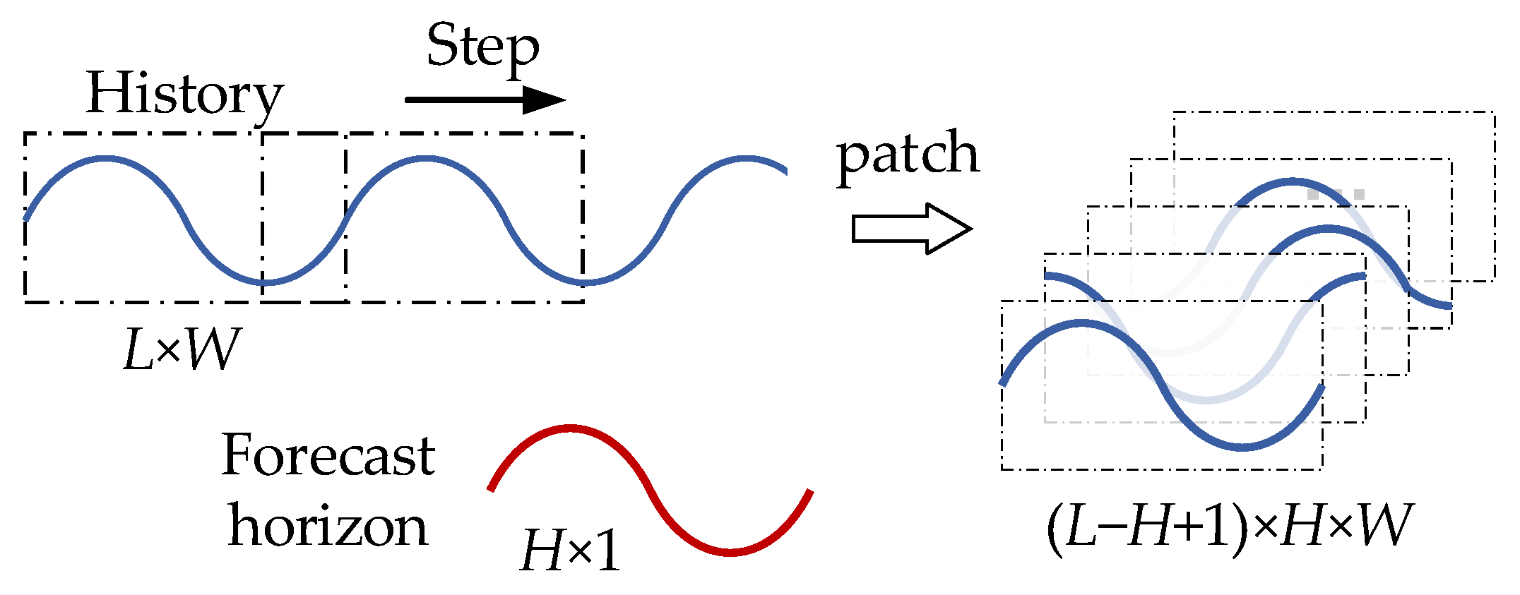
3.2. Patch Squeeze and Excitation Module

An attention module called patch squeeze and excitation (PSE) is proposed to effectively extract information hidden in both static and dynamic variables by focusing on different segments and features of historical data. The PSE module has two parts: the first part, called the patch, segments historical information into fixed-length slices using a technique similar to the sliding window approach. Patch aims to divide the historical data into segments matching the length of the forecast horizon, assuming that some segments exhibit similar patterns to the forecast horizon data, as long as the historical data is sufficiently long (at least longer than the forecast horizon). In subsequent processing, segments with higher similarity are focused on to reduce redundancy in the information. Patch includes two hyperparameters: stride and width. The stride is set to a minimum value of 1 to ensure sufficient resolution during segmentation and prevent the omission of any segments similar to the forecast data. The width is equal to the forecast horizon, ensuring that similarity segments are searched only within the range of interest. Obviously, the range of interest corresponds to the forecast horizon. An excessively large or small width can distract from attention and reduce search effectiveness. The principle of patch is illustrated in Figure 2.

The patch operation results in $L-H+1$ slices, each with a length of H. Certain slices are thought to contain components similar to the forecast target and therefore deserve special attention. To address this, the squeeze and excitation (SE) attention module is introduced to calculate the importance of each slice [39]. The main idea of SE is to extract a global representation of channel information through squeezing and then adaptively assign weights to channels via excitation, distinguishing the importance of information in each channel. The original SE module employs global average pooling to capture the information strength of each channel. Building on this, a local metric is proposed to assess the information strength of slice details across various dimensions.

Let $u_s\left(i,j\right)$ denote the value of slice s at the i-th time step and the j-th feature. The global representation of slice s, derived from average pooling, is expressed as:

$$a_s={\displaystyle \frac{1}{H\times W}}{\displaystyle \sum _{i=1}^H{\displaystyle \sum _{j=1}^W{u}_s\left(i,j\right)}}$$

(7)

Average pooling along the time dimension yields the local information strength of each feature in slice s, represented as:

$$T{A}_s\left(j\right)={\displaystyle \frac{1}{H}}{\displaystyle \sum _{i=1}^H{u}_s\left(i,j\right)}$$

(8)

Adaptive weights ${\mathit{w}}_t$ (from a trainable fully connected layer) are used to fuse local information $T{A}_s\left(j\right)$, producing an indicator $t_s$ for the information strength of slice s, expressed as:

$$t_s={\mathit{w}}_t\cdot \mathit{T}{\mathit{A}}_s^T+b_t$$

(9)

Average pooling along the feature dimension yields the local information strength of each time step in slice s, represented as:

$$F{A}_s\left(i\right)={\displaystyle \frac{1}{W}}{\displaystyle \sum _{j=1}^W{u}_s\left(i,j\right)}$$

(10)

Similarly, adaptive weights ${\mathit{w}}_f$ (obtained from a trainable fully connected layer) are used to fuse the local information $F{A}_s\left(i\right)$, resulting in an indicator $f_s$ that represents the information strength of slice s, expressed as follows:

$$f_s={\mathit{w}}_f\cdot \mathit{F}{\mathit{A}}_s^T+b_f$$

(11)

The indicator that represents the information strength of slice s can be derived from the three components mentioned above,

$$z_s=a_s+t_s+f_s$$

(12)

After obtaining the global information embedding, the excitation operation in SE comprehensively captures channel dependencies and derives an importance measure for each slice. This is implemented using two fully connected layers, which can be expressed as:

$$\mathit{e}={\mathrm{F}}_{ex}\left(\mathit{z},\mathit{w}\right)=\sigma \left({\mathit{w}}_2\left(\delta \left({\mathit{w}}_{1}z+b_1\right)\right)+b_2\right)$$

(13)

where $\delta \left(\cdot \right)$ is the rectified linear unit activation function.

The importance vector $\mathit{e}$ of the slice is used to perform weighted fusion of all slices from the sample, resulting in more aggregated information ${\mathit{x}}^{\prime }$,

$${\mathit{x}}^{\prime }={\displaystyle \sum _{s=1}^S{e}_s{\mathit{u}}_s}$$

(14)

3.3. Algorithm Implementation

This paper presents a multi-step probabilistic forecasting method for time series, as illustrated in Figure 3. First, the stacked historical review information ${\mathit{y}}_{i,1:T}$ and covariates $x_{i,1:T}$ serve as the input to the PSE module. After passing through the PSE module, redundant information is eliminated, enabling the LSTM to more effectively extract the temporal dependencies of the sequence. The LSTM output ${\mathit{h}}_i$ is processed through multiple fully connected layers to obtain the parameters $\mathit{\theta }$ of the distribution function for future time steps. Assuming a Gaussian distribution, the parameters $\mathit{\mu }$ serve as the forecasts, while $\mathit{\sigma }$ are used to calculate the confidence interval. Under other distribution assumptions, sufficient samples can be obtained by sampling from the assumed distribution, allowing for the calculation of quantile information to facilitate probabilistic forecasting. Additionally, the quantile regression method uses the hidden states ${\mathit{h}}_i$ of LSTM, processed through fully connected layers, to yield predictions for various quantiles.

3.4. Probabilistic Forecasting

Two probabilistic forecasting frameworks are proposed to realize the diverse demand forecasting tasks in the real world, such as lead-time demand forecasting and continuous short-, medium-, and long-term forecasting. Parametric forecasting methods use maximum likelihood estimation to obtain the parameters of an assumed distribution for future observations, such as the variance and mean of a Gaussian distribution, providing high adaptability and flexibility. Estimates and intervals for future observations can be obtained by randomly sampling from these distributions. Additionally, their parameters can be directly used as predictions. For example, the mean of a Gaussian distribution serves as the expected forecast, while the variance indicates uncertainty. In contrast, non-parametric methods do not require distribution assumptions and generate prediction intervals for future observations using quantile regression, which offers greater robustness.

3.4.1. Parametric Approach

Parametric methods require prior assumptions about the distribution based on the statistical characteristics of the data, followed by maximum likelihood estimation to obtain the parameters of this assumed distribution. This model outputs a set of parameters for each time step of the future observation ${\mathit{y}}_{i,T+1:T+H}$, for example, the mean ${\mathit{\mu }}_{i,T+1:T+H}$ and variance ${\mathit{\sigma }}_{i,T+1:T+H}$ of the Gaussian distribution. The negative log-likelihood function is used as the optimization objective (loss function) for the model, as expressed below:

$$\begin{array}{ll}{ℒ}_G& ={\displaystyle \sum _i\left(-\log {\displaystyle \prod _{h=1}^{H}p\left(\cdot \left|{\theta }_{i,h}\left({\mathit{h}}_i,\Theta \right)\right.\right)}\right)}\\ & ={\displaystyle \sum _i\left(-{\displaystyle \sum _{h=1}^H\log \left({\left(2\pi {\sigma }_{i,h}^2\right)}^{-1/2}\exp \left[-{\left(y_{i,h}-{\mu }_{i,h}\right)}^2/\left(2{\sigma }_{i,h}^2\right)\right]\right)}\right)}\\ & ={\displaystyle \sum _i\left({\displaystyle \sum _{h=1}^H\left(\frac{1}{2}\log \left(2\pi \right)+\log \left({\sigma }_{i,h}\right)+\frac{{\left(y_{i,h}-{\mu }_{i,h}\right)}^2}{2{\sigma }_{i,h}^2}\right)}\right)}\end{array}$$

(15)

This approach can be extended to other distribution functions, such as the negative binomial distribution for modeling positive count sequences [33,40] and the Bernoulli distribution for binary data [41]. It is important to note that some parameters of these distributions must meet positivity constraints, such as the variance of the Gaussian distribution; to achieve this, a softplus activation function is used,

$$softplus\left(x\right)=\log \left(1+e^x\right)$$

(16)

3.4.2. Non-Parametric Approach

The quantile regression is used to generate predicted quantiles and prediction intervals for future observations. Quantile regression minimizes the quantile loss between the predicted values ${\widehat{y}}^q$ and the actual values y at a given quantile level q, as expressed below:

$${ℒ}_q\left({\widehat{y}}^q,y\right)=\left\{\begin{array}{cc}q\left(y-{\widehat{y}}^q\right)& {\widehat{y}}^q\le y\\ \left(1-q\right)\left({\widehat{y}}^q-y\right)& {\widehat{y}}^q>y\end{array}\right.$$

(17)

Changing the value of q enables predictions at various quantile levels. Given a set of quantiles $\left\{q_1,q_2,\dots ,q_n\right\}$, minimizing the total quantile loss yields n quantile predictions, allowing for various interval forecasts.

$${ℒ}_Q={\displaystyle \sum _{i=1}^n{ℒ}_{qi}\left({\widehat{y}}^{qi},y\right)}$$

(18)

4. Experimental Setup and Results

In this section, comparison experiments are conducted to demonstrate the superiority of the proposed method. All experiments were conducted on a CentOS 9 system with an NVIDIA GeForce RTX 4090 GPU, utilizing the PyTorch 1.3 deep learning framework.

4.1. Data Preparation

4.1.1. Data Description

Electricity is one of the most critical inputs for process industries; power load forecasting can optimize production, conserve energy, and improve efficiency. Thus, an open-access electricity load dataset [42] is used for experimental analysis. This classic univariate dataset in power load forecasting contains electricity usage data every 15 min (measured in kW) from 370 users, spanning the period from 2011 to 2014. Details are provided in

Table 2. Dataset description and statistics.

Parameter	Values
# of time series	370
granularity	per 15 min
time scope	1 January 2011 00:15:00 to 1 January 2015 00:00:00
backtracking history	192
forecast horizon	24, 48
domain	$\text{ℝ}$

.

Diversity in electricity demand and consumption behavior among users results in complex power load patterns. Consequently, addressing amplitude differences is essential for building a global predictor for all series. Moreover, because the time granularity of this dataset is relatively fine, we need to convert it into an hourly sampled electricity series to decrease resource consumption. Therefore, some preprocessing steps on the data are essential.

4.1.2. Data Preprocessing

The original electricity data are converted into a load series with one measurement per hour by summing the data as recommended in the dataset description. Each summed load value was divided by four to convert values to kWh [42]. Besides the electricity load, some artificial features, including hour, weekday, and day of month, are extracted from the timestamp to capture the location information of each observation. Sine and cosine encoding are applied to these artificial features, detailed below:

$$\left\{\begin{array}{l}po{s}_{\sin }=\sin \left(2\pi s_i/S\right)\\ po{s}_{\cos }=\cos \left(2\pi s_i/S\right)\end{array}\right.$$

(19)

where, $s_i$ is the i-th value of the artificial feature. S denotes seasonality. For ‘hour’, it is 24; for ‘day of the week’, it is 7; and for ‘day of the month’, the range is 28 to 31.

Data from 1 January 2011 00:01:00 to 31 December 2013 23:00:00 are used as the training set (about 75% of total data points), data from 1 January 2014 00:00:00 to 30 June 2014 23:00:00 are used as the validation set (about 12.5% of total data points), and data from 1 July 2014 00:00:00 to 31 December 2014 23:00:00 are used for performance testing (about 12.5% of total data points). To account for significant fluctuations in power consumption data among users, the min-max normalization method is applied to scale all series and ensure the algorithm’s effectiveness, as shown in the following formula:

$${\widehat{x}}_i^{\left(j\right)}={\displaystyle \frac{x_i^{\left(j\right)}-x_{\min }^{\left(j\right)}}{x_{\max }^{\left(j\right)}-x_{\min }^{\left(j\right)}}}$$

(20)

where, $x_i^{\left(j\right)}$ denotes the i-th observation in the j-th time series; ${\widehat{x}}_i^{\left(j\right)}$ denotes the normalized data of $x_i^{\left(j\right)}$; $x_{\max }^{\left(j\right)}$ and $x_{\min }^{\left(j\right)}$ denote the maximum and minimum values of all observations in the j-th time series, respectively. Actually, the minimum and maximum values of training set are used to normalize both the training and testing sets, preventing future information from leaking into the past.

The sliding window technique is applied to divide the data from the training set, validation set and test set into independent instances. The window width settings are provided in Table 1.

4.1.3. Performance Metrics

Four evaluation metrics were applied to quantitatively assess the performance of all methods used in the experiments. Prediction interval coverage probability (PICP) [23] evaluates how well the prediction interval covers the true values. This is a positive indicator; a higher PICP means a greater probability that the true value lies within the interval. It is defined as:

$$PICP={\displaystyle \frac{1}{N}}{\displaystyle \sum _{i=1}^N{c}_i}$$

(21)

where, $c_i$ is a binary variable that indicates whether the true value $y_i$ lies within the prediction interval. Let $U_i$ denote the upper bound and $L_i$ the lower bound of the prediction interval; $c_i$ is defined as follows:

$$c_i=\left\{\begin{array}{l}1,y_i\in \left[L_i,U_i\right]\\ 0,other\end{array}\right.$$

(22)

Prediction interval normalized averaged width (PINAW) [23] assesses the narrowness of the prediction interval. Typically, a narrower prediction interval conveys more information and practical value, defined as follows:

$$PINAW={\displaystyle \frac{1}{NR}}{\displaystyle \sum _{i=1}^N\left(U_i-L_i\right)}$$

(23)

where, R represents the range of the true values $y_i$ on the forecast horizon.

Symmetric mean absolute percentage error (sMAPE) [34] evaluates the shape error between predicted and actual values. This is a negative indicator: a smaller value signifies that the predicted curve is closer to the actual curve, defined as follows:

$$sMAPE={\displaystyle \frac{2}{N}}{\displaystyle \sum _{i=1}^N\frac{\left|{\widehat{y}}_i-y_i\right|}{\left|{\widehat{y}}_i\right|+\left|y_i\right|}}$$

(24)

where, ${\widehat{y}}_i$ denotes predicted values. To avoid both the predicted value ${\widehat{y}}_i$ and the true value $y_i$ being zero, a small constant $\epsilon$ is typically added to the predicted values ${\widehat{y}}_i$ during implementation.

Normalized deviation (ND) [33] assesses the deviation between predicted and true values. This is a negative indicator: a smaller value signifies better performance, defined as follows:

$$ND={\displaystyle \frac{{\displaystyle \sum _{i=1}^N\left|{\widehat{y}}_i-y_i\right|}}{{\displaystyle \sum _{i=1}^N\left|y_i\right|}}}$$

(25)

4.2. Comparison Experiments

A series of comparative and ablation experiments are conducted to verify the effectiveness of the proposed method. These comparative methods are described briefly as follows:

LSTM: The foundational model for all methods in the experimental section, which enables point predictions across various forecast horizons.

PSE-LSTM-Gaussian: The proposed method predicts expected future observations using the Gaussian likelihood distribution parameter $\mu$ and manages uncertainty with the distribution parameter $\sigma$.

PSE-LSTM-quantile: The proposed method generates different quantile predictions for future observations through quantile regression.

LSTM-Gaussian: This method employs LSTM as the base, retaining the same structure as the proposed method except for the PSE module, to validate its effectiveness.

LSTM-quantile: This method serves as an ablation experiment to validate the effectiveness of the PSE module.

DeepAR-Gaussian [33]: This method utilizes LSTM for maximum likelihood estimation of assumed distribution parameters and then samples from the distribution to make predictions.

In the Gaussian-based method, the distribution parameter μ is used as the predicted value to calculate the ND and sMAPE metrics, while σ is used to compute the PICP and PINAW metrics based on symmetric intervals around the mean μ. For the quantile-based method, the 50th quantile serves as the predicted value for calculating ND and sMAPE metrics, while the 10th and 90th quantile intervals are used for PICP and PINAW metrics. All methods employ the Adam optimizer for gradient calculation and are run for 50 epochs. Grid search is used to identify the optimal hyperparameters; for additional hyperparameter optimization methods, please refer to [43,44]. The key hyperparameters are specified in

Table 3. Hyperparameter settings.

	Hidden Node	Hidden Layer	Learning Rate
LSTM	128	2	0.01
LSTM-Gaussian	128	2	0.001
LSTM-quantile	128	2	0.01
DeepAR-Gaussian	40	2	0.001
PSE-LSTM-Gaussian	128	2	0.001
PSE-LSTM-quantile	128	2	0.01

.

The experiments of 24-h-ahead and 48-h-ahead predictions are conducted to evaluate the metrics performance of each method, with the results shown in

Table 4. Performance comparison of the proposed method with other methods.

Forecast Horizon		24				48
Method	Metric	PICP↑	PINAW↓	ND↓	sMAPE↓	PICP↑	PINAW↓	ND↓	sMAPE↓
LSTM		-	-	0.117	0.167	-	-	0.118	0.174
LSTM-Gaussian		0.971	1.931	0.120	0.163	0.974	1.567	0.121	0.168
LSTM-quantile		0.795	0.770	0.115	0.154	0.792	0.499	0.106	0.144
DeepAR-Gaussian		0.974	2.221	0.128	0.183	0.964	1.542	0.142	0.188
PSE-LSTM-Gaussian		0.980	1.166	0.082	0.120	0.978	0.938	0.093	0.133
PSE-LSTM-quantile		0.786	0.423	0.082	0.121	0.768	0.331	0.088	0.125

. The best performance results are highlighted in bold. Arrows (↑ and ↓) following each metric indicate directional preference: ↑ means higher values are better, and ↓ means lower values are preferable. Compared to both point prediction and probability prediction baselines, the proposed methods (PSE-LSTM-Gaussian and PSE-LSTM-quantile) achieve the best performance metrics, demonstrating their superiority. All probabilistic forecasting methods demonstrate performance comparable to or better than the benchmark method (LSTM) in point prediction evaluation metrics (ND and sMAPE), indicating their effectiveness in point prediction tasks. Probabilistic forecasting provides additional information on future uncertainties, allowing for the generation of potential intervals and probability distributions for future observations—capabilities not available with point predictions. Thus, the application scenarios for probabilistic forecasting are broader than those for point predictions. Moreover, compared to methods like DeepAR-Gaussian, which achieve multi-step predictions recursively, LSTM-Gaussian and PSE-LSTM-Gaussian directly output multi-step prediction results, demonstrating higher performance. This provides strong evidence that multi-step predictions can avoid the gradual accumulation of errors.

The comparisons of the proposed PSE-LSTM-Gaussian with LSTM-Gaussian, and PSE-LSTM-quantile with LSTM-quantile, demonstrate the effectiveness of the PSE module presented in this paper. By assigning varying levels of attention to slice information during historical backtracking, the model’s performance can be improved, making predicted expectations closer to true values. Additionally, it effectively reduces the width of the prediction interval without significantly decreasing coverage, thus providing practitioners with refined insights for managing uncertainty. Therefore, this paper recommends that readers use PSE techniques to preprocess data when performing their tasks.

To further illustrate the predictive performance of various methods in the experiments, we randomly selected a test sample at different forecast horizons and plotted the results, as shown in Figure 4. The proposed method’s predicted expectations are most consistent with changes in the true load among all methods and have the narrowest prediction interval. Furthermore, non-recursive methods can effectively track changes in true load, with predicted expectations closer to the actual load, better reflecting its peaks and troughs. In contrast, predictions from recursive methods are smoother, reflecting the overall fluctuation trend of true load, but they lack sufficient resolution in detail. In the real world, high-frequency data, such as demand and load recorded hourly or daily, often contain many random components, leading to noticeable fluctuations that recursive methods struggle to handle effectively. However, as data are aggregated to higher levels, such as monthly, quarterly, or yearly statistics, the amplitude is amplified through summation, making fluctuations less significant relative to the data scale. With less emphasis on data details, recursive methods tend to perform better in aggregated forecasts.

Additionally, Table 4 shows that the parametric method based on the Gaussian distribution and the non-parametric method based on quantile regression yield similar results for point prediction metrics. However, significant differences exist in the evaluation metrics for probabilistic predictions. To explore this discrepancy, we plotted a comparative chart of the experimental results from both methods, as shown in Figure 5. The plotted results show that while the quantile regression method has a narrower prediction interval, it does not include all true values across the prediction horizon. For example, the true values indicated by the black dashed rectangle in the figure are not included in the quantile prediction interval. In quantile regression, the 80% confidence interval is defined as the prediction interval between the 10th and 90th percentiles, indicating an 80% probability that the true value falls within this interval, which closely matches the PICP value in Table 4. In contrast, the Gaussian-based method uses the range of the $\mu \pm \sigma$ as the prediction interval. Although the confidence level for this interval cannot be calculated, the PICP indicator for the Gaussian-based method indicates that it covers at least 97% of true values. However, we cannot conclude that the Gaussian-based method is superior to the quantile regression method, as they serve different scenarios, and users should choose based on their specific task requirements.

Lowering the confidence requirement theoretically permits narrower prediction intervals. The PICP values for various prediction intervals based on the Gaussian method are calculated to explore confidence level variations. The prediction intervals were constructed using different multiples of the σ parameter from the model’s predicted Gaussian distribution, as shown in Figure 6. Selecting 0.4 times σ to construct the prediction interval achieves an approximate 80% confidence level, recommended for many task scenarios. Additionally, choosing larger multiples (greater than 1) does not significantly increase PICP as the prediction interval range expands; therefore, larger multiples are not recommended.

5. Discussion and Conclusions

A probabilistic time series forecasting method is proposed to tackle the challenge of constructing global forecasting models, due to significant amplitude fluctuations and complex patterns in large-scale time series data. The PSE module is used to assess the influence of historical data on future observations, both globally and in detail, enhancing forecasting accuracy. Additionally, both parametric and non-parametric forecasting methods are provided to perform multi-step probabilistic predictions. The proposed method is validated by a multi-user electricity load dataset. Probabilistic forecasts based on assumed distributions and those based on quantile regression achieve similar point prediction accuracy but differ significantly in their prediction intervals. Users can select the appropriate implementation flexibly based on task requirements. In experiments exploring the performance of the parametric method based on assumed distributions for predicting intervals, we found that constructing prediction intervals with lower multiples of the Gaussian distribution variance (<0.4) results in a nearly linear change in confidence level with respect to the confidence interval. The confidence interval at 0.4 times the variance σ corresponds to an approximately 80% confidence level, whereas using larger multiples does not yield significant improvements.

Determining the distribution of non-stationary data is challenging. If the assumed distribution significantly deviates from the actual distribution, forecasting accuracy can be severely impacted. While methods assuming a Gaussian distribution have shown some success in power load forecasting, this assumption may not generalize to other time series, nor can we confirm that alternative distributions would yield better results—a limitation of this study. Many distributional assumptions in research rely on subjective experience, which can introduce considerable cognitive bias. Thus, exploring adaptive distribution methods based on historical data patterns to reduce cognitive bias is worthwhile. Additionally, using non-parametric methods to reconstruct probability density functions is also an approach to reduce subjective error.

References

1. Burke, I.; Salzer, S.; Stein, S.; Olusanya, T.O.O.; Thiel, O.F.; Kockmann, N. AI-Based Integrated Smart Process Sensor for Emulsion Control in Industrial Application. Processes 2024, 12, 1821. [Google Scholar] [CrossRef]
2. Liu, S.; Papageorgiou, L.G. Multiobjective optimisation of production, distribution and capacity planning of global supply chains in the process industry. Omega 2013, 41, 369–382. [Google Scholar] [CrossRef]
3. Yi, K.; Zhang, Q.; Fan, W.; Wang, S.; Wang, P.; He, H.; Niu, Z. Frequency-domain MLPs are more effective learners in time series forecasting. Adv. Neural Inf. Process. Syst. 2024, 36, 76656–76679. [Google Scholar]
4. He, Q.Q.; Wu, C.; Si, Y.-W. LSTM with particle Swam optimization for sales forecasting. Electron. Commer. Res. Appl. 2022, 51, 101118. [Google Scholar] [CrossRef]
5. Huang, J.; Chen, Q.; Yu, C. A new feature based deep attention sales forecasting model for enterprise sustainable development. Sustainability 2022, 14, 12224. [Google Scholar] [CrossRef]
6. Jiang, B.; Liu, Y.; Geng, H.; Wang, Y.; Zeng, H.; Ding, J. A holistic feature selection method for enhanced short-term load forecasting of power system. IEEE Trans. Instrum. Meas. 2023, 72, 2500911. [Google Scholar] [CrossRef]
7. Zhang, W.; Lin, Z.; Liu, X. Short-term offshore wind power forecasting-A hybrid model based on Discrete Wavelet Transform (DWT), Seasonal Autoregressive Integrated Moving Average (SARIMA), and deep-learning-based Long Short-Term Memory (LSTM). Renew. Energy 2022, 185, 611–628. [Google Scholar] [CrossRef]
8. Zhang, Z.; Li, M.; Lin, X.; Wang, Y.; He, F. Multistep speed prediction on traffic networks: A deep learning approach considering spatio-temporal dependencies. Transp. Res. Part C Emerg. Technol. 2019, 105, 297–322. [Google Scholar] [CrossRef]
9. Hu, M.; Li, H.; Song, H.; Li, X.; Law, R. Tourism demand forecasting using tourist-generated online review data. Tour Manag. 2022, 90, 104490. [Google Scholar] [CrossRef]
10. Croston, J.D. Forecasting and Stock Control for Intermittent Demands. J. Oper. Res. Soc. 1972, 23, 289–303. [Google Scholar] [CrossRef]
11. Syntetos, A.A.; Boylan, J.E. On the bias of intermittent demand estimates. Int. J. Prod. Econ. 2001, 71, 457–466. [Google Scholar] [CrossRef]
12. Teunter, R.H.; Syntetos, A.A.; Zied Babai, M. Intermittent demand: Linking forecasting to inventory obsolescence. Eur. J. Oper. Res. 2011, 214, 606–615. [Google Scholar] [CrossRef]
13. Chatfield, C. The Holt-winters forecasting procedure. J. R. Stat. Soc. Ser. C (Appl. Stat.) 1978, 27, 264–279. [Google Scholar] [CrossRef]
14. Ray, S.; Lama, A.; Mishra, P.; Biswas, T.; Das, S.S.; Gurung, B. An ARIMA-LSTM model for predicting volatile agricultural price series with random forest technique. Appl. Soft Comput. 2023, 149, 110939. [Google Scholar] [CrossRef]
15. Tarmanini, C.; Sarma, N.; Gezegin, C.; Ozgonenel, O. Short term load forecasting based on ARIMA and ANN approaches. Energy Rep. 2023, 9, 550–557. [Google Scholar] [CrossRef]
16. Kochetkova, I.; Kushchazli, A.; Burtseva, S.; Gorshenin, A. Short-term mobile network traffic forecasting using seasonal ARIMA and holt-winters models. Future Internet 2023, 15, 290. [Google Scholar] [CrossRef]
17. Liu, X.; Lin, Z.; Feng, Z. Short-term offshore wind speed forecast by seasonal ARIMA-A comparison against GRU and LSTM. Energy 2021, 227, 120492. [Google Scholar] [CrossRef]
18. Bi, J.-W.; Liu, Y.; Li, H. Daily tourism volume forecasting for tourist attractions. Ann. Tour. Res. 2020, 83, 102923. [Google Scholar] [CrossRef]
19. Li, J.; Deng, D.; Zhao, J.; Cai, D.; Hu, W.; Zhang, M.; Huang, Q. A novel hybrid short-term load forecasting method of smart grid using MLR and LSTM neural network. IEEE Trans. Ind. Inform. 2020, 17, 2443–2452. [Google Scholar] [CrossRef]
20. Andrade, L.A.C.G.; Cunha, C.B. Disaggregated retail forecasting: A gradient boosting approach. Appl. Soft Comput. 2023, 141, 110283. [Google Scholar] [CrossRef]
21. Zhou, H.; Dang, Y.; Yang, Y.; Wang, J.; Yang, S. An optimized nonlinear time-varying grey Bernoulli model and its application in forecasting the stock and sales of electric vehicles. Energy 2023, 263, 125871. [Google Scholar] [CrossRef]
22. Ma, S.; Fildes, R. Retail sales forecasting with meta-learning. Eur. J. Oper. Res. 2021, 288, 111–128. [Google Scholar] [CrossRef]
23. Bracale, A.; Caramia, P.; De Falco, P.; Hong, T. Multivariate quantile regression for short-term probabilistic load forecasting. IEEE Trans. Power Syst. 2019, 35, 628–638. [Google Scholar] [CrossRef]
24. Papacharalampous, G.; Langousis, A. Probabilistic water demand forecasting using quantile regression algorithms. Water Resour. Res. 2022, 58, e2021WR030216. [Google Scholar] [CrossRef]
25. Wang, J.; Wang, S.; Zeng, B.; Lu, H. A novel ensemble probabilistic forecasting system for uncertainty in wind speed. Appl. Energy 2022, 313, 118796. [Google Scholar] [CrossRef]
26. Wang, K.; Zhang, Y.; Lin, F.; Wang, J.; Zhu, M. Nonparametric probabilistic forecasting for wind power generation using quadratic spline quantile function and autoregressive recurrent neural network. IEEE Trans. Sustain. Energy 2022, 13, 1930–1943. [Google Scholar] [CrossRef]
27. Jensen, V.; Bianchi, F.M.; Anfinsen, S.N. Ensemble conformalized quantile regression for probabilistic time series forecasting. IEEE Trans. Neural Netw. Learn. Syst. 2022, 35, 9014–9025. [Google Scholar] [CrossRef]
28. Luo, L.; Dong, J.; Kong, W.; Lu, Y.; Zhang, Q. Short-Term Probabilistic Load Forecasting Using Quantile Regression Neural Network with Accumulated Hidden Layer Connection Structure. IEEE Trans. Ind. Informatics. 2024, 20, 5818–5828. [Google Scholar] [CrossRef]
29. Ryu, S.; Yu, Y. Quantile-mixer: A novel deep learning approach for probabilistic short-term load forecasting. IEEE Trans. Smart Grid. 2024, 15, 2237–2250. [Google Scholar] [CrossRef]
30. Wen, H. Probabilistic wind power forecasting resilient to missing values: An adaptive quantile regression approach. Energy 2024, 300, 131544. [Google Scholar] [CrossRef]
31. Chen, Y.; He, Y.; Xiao, J.W.; Wang, Y.W.; Li, Y. Hybrid model based on similar power extraction and improved temporal convolutional network for probabilistic wind power forecasting. Energy 2024, 304, 131966. [Google Scholar] [CrossRef]
32. Grecov, P.; Prasanna, A.N.; Ackermann, K.; Campbell, S.; Scott, D.; Lubman, D.I.; Bergmeir, C. Probabilistic causal effect estimation with global neural network forecasting models. IEEE Trans. Neural Netw. Learn. Syst. 2024, 35, 4999–5013. [Google Scholar] [CrossRef] [PubMed]
33. Salinas, D.; Flunkert, V.; Gasthaus, J.; Januschowski, T. DeepAR: Probabilistic forecasting with autoregressive recurrent networks. Int. J. Forecast. 2020, 36, 1181–1191. [Google Scholar] [CrossRef]
34. Chen, Y.; Kang, Y.; Chen, Y.; Wang, Z. Probabilistic forecasting with temporal convolutional neural network. Neurocomputing 2020, 399, 491–501. [Google Scholar] [CrossRef]
35. Sun, M.; Feng, C.; Zhang, J. Multi-distribution ensemble probabilistic wind power forecasting. Renew. Energy 2020, 148, 135–149. [Google Scholar] [CrossRef]
36. Olivares, K.G.; Meetei, O.N.; Ma, R.; Reddy, R.; Cao, M.; Dicker, L. Probabilistic hierarchical forecasting with deep poisson mixtures. Int. J. Forecast. 2024, 40, 470–489. [Google Scholar] [CrossRef]
37. Rügamer, D.; Baumann, P.F.M.; Kneib, T.; Hothorn, T. Probabilistic time series forecasts with autoregressive transformation models. Stat. Comput. 2023, 33, 37. [Google Scholar] [CrossRef]
38. Qiao, L.; Gao, H.; Cui, Y.; Yang, Y.; Liang, S.; Xiao, K. Reservoir Porosity Construction Based on BiTCN-BiLSTM-AM Optimized by Improved Sparrow Search Algorithm. Processes 2024, 12, 1907. [Google Scholar] [CrossRef]
39. Hu, J.; Shen, L.; Sun, G. Squeeze-and-excitation networks. In Proceedings of the IEEE Conference on Computer Vision and Pattern Recognition, Salt Lake City, UT, USA, 18–22 June 2018; pp. 7132–7141. [Google Scholar]
40. Sillanpää, V.; Liesiö, J. Forecasting replenishment orders in retail: Value of modelling low and intermittent consumer demand with distributions. Int. J. Prod. Res. 2018, 56, 4168–4185. [Google Scholar] [CrossRef]
41. Berry, L.R.; Helman, P.; West, M. Probabilistic forecasting of heterogeneous consumer transaction–sales time series. Int. J. Forecast. 2020, 36, 552–569. [Google Scholar] [CrossRef]
42. Trindade, A. ElectricityLoadDiagrams20112014. 2015. UCI Machine Learning Repository. Available online: https://archive.ics.uci.edu/dataset/321/electricityloaddiagrams20112014 (accessed on 25 January 2024).
43. Hanifi, S.; Cammarono, A.; Zare-Behtash, H. Advanced hyperparameter optimization of deep learning models for wind power prediction. Renew. Energy 2024, 221, 119700. [Google Scholar] [CrossRef]
44. Calik, N.; Güneş, F.; Koziel, S.; Pietrenko-Dabrowska, A.; Belen, M.A.; Mahouti, P. Deep-learning-based precise characterization of microwave transistors using fully-automated regression surrogates. Sci. Rep. 2023, 13, 1445. [Google Scholar] [CrossRef] [PubMed]
Figure 1. The structure of the LSTM cell unit.
Processes 12 02700 g001
Figure 2. The illustration of patch.
Processes 12 02700 g002
Figure 3. The flowchart of using the proposed method.
Processes 12 02700 g003
Figure 4. The prediction results of the Gaussian-based methods. The black line represents the true target. The colored dashed lines represent the predicted expectations of various methods, while the shaded areas indicate the prediction intervals, which are symmetric intervals around the predicted expectations with a radius of σ.
Processes 12 02700 g004
Figure 5. Comparison of results between the Gaussian-based method and the quantile regression method. The solid line represents the true values, while the dashed lines show the predicted values from various methods. The shaded areas indicate the prediction intervals for these methods. The dashed box highlights true values that are not covered by the prediction intervals.
Processes 12 02700 g005
Figure 6. PICP of different prediction intervals based on the Gaussian distribution method.
Processes 12 02700 g006