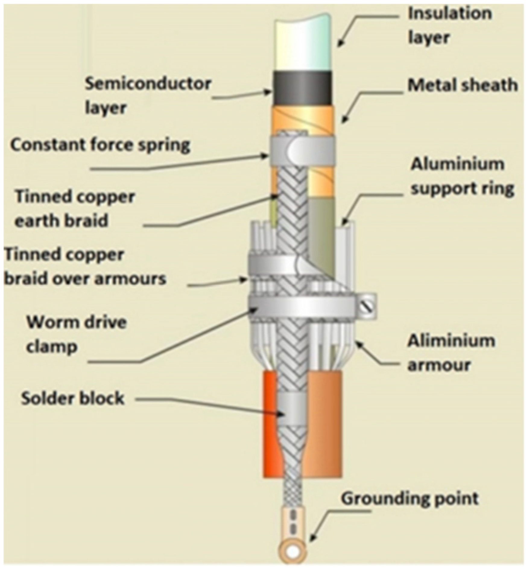
Article

Optimum Cable Bonding with Pareto Optimal and Hybrid Neural Methods to Prevent High-Voltage Cable Insulation Faults in Distributed Generation Systems

Electric Electronic Engineering Department, Engineering Faculty, Aksaray University, Aksaray 68100, Turkey
Processes 2024, 12(12), 2909; https://doi.org/10.3390/pr12122909
Submission received: 25 November 2024 / Revised: 15 December 2024 / Accepted: 17 December 2024 / Published: 19 December 2024
(This article belongs to the Special Issue Fault Diagnosis of Equipment in the Process Industry)

Abstract

:
The high voltage, current and harmonic distortion in high-voltage cable metal sheaths cause cable insulation faults. The SSBLR (Sectional Solid Bonding with Inductance (L) and Resistance) method was designed as a new cable grounding method to prevent insulation faults. SSBLR was optimized using multi-objective optimization (MOP) with the prediction method (PM) to minimize these factors. The Pareto optimal method was used for MOP. The artificial neural network, hybrid artificial neural network and regression methods were used as the PM. When the artificial neural network–genetic algorithm hybrid method was used as the PM, and the genetic algorithm was used as the optimization method, the voltage and current were significantly reduced in the metal sheath of the cable.

1. Introduction

High-voltage cable faults are an important factor in terms of the sustainability of electrical energy. High-voltage cables consist of different layers. These layers are shown in Figure 1 [1]. The most important layer is the insulation layer because the insulation layer prevents short circuits by insulating the phase conductor.
However, an increase in the temperature of the insulation layer weakens the electric strength of the insulation material [2]. If the insulation material in the insulation layer weakens, it can be punctured by the electrical field. Hence, a cable insulation fault occurs [3,4,5].
The insulation layer is covered with a metal sheath as shown in Figure 1. If the current flows through the metal sheath, the temperature of the insulation layer increases. The metal sheath is grounded to restrict high electrical stress. However, when the metal parts of the cable are grounded the sheath current (SC) flows in these metal parts. Also, the SC can be up to 50% of line current. The unbalanced line current is one of the most important factors in the formation of the sheath current. The unbalanced current flows from the neutral points of the transformers to the ground and is called zero sequence current.
The cable configuration is another factor in the formation of the zero sequence current. Even if the line currents are balanced, the zero sequence current occurs in the metal parts of the cable owing to the cable configuration. For example, an 800 A sheath current occurs in the metal part of 30 km high-voltage cable in wind farm [6,7,8]. The cable configurations shown are trefoil and flat. These arrangements are shown in Figure 2.
In addition, when phase-to-ground short circuit faults or unbalanced line currents occur between the transformer substations, the zero sequence current flows between the neutral points of the transformers. If there is high-ground resistance between the transformer substations, the zero sequence current flows in the metal sheath of the cable instead of the ground. This situation is shown in Figure 3.
As can be seen from Figure 3, high-voltage cables are grounded at the line’s head and end. In this case, the zero sequence current flows through the metal sheath of the high-voltage cables, so the sheath voltage increases at the cable termination points. Thus, a potential tent occurs at the cable termination points. If the grounding resistances of the line head and the line end are different from each other, the potential tents in these regions are different from each other. Therefore, the high voltage is carried to the line head or line end as potential drift. This case causes a lot of energy loss on the high-voltage line, and it also causes an increase in temperature in the cable [9]. The cable temperature according to the SC is shown in Table 1.
In particular, if there are current harmonics in the sheath current, the temperature of the insulation layer increases excessively because of the high-frequency current harmonics [10]. Namely, one of the most important factors in the increase in the temperature of cable insulation is the current harmonics. In addition, harmonics cause resonance and a high voltage in the insulation layer [11].
The main reason for harmonic distortion in electrical networks is the use of power electronic elements. Renewable energy sources are the most important harmonic sources because power electronic elements are used for the conversion of DC/AC in renewable energy sources. Renewable energy sources can be photovoltaic power plants, wind power plants and biofuel facilities. Distributed generation plants (DGPs) are formed by using these facilities together. Distributed generation plants play an important role in the stability of electrical networks. However, distributed generation plants cause current and voltage harmonics [12,13,14,15,16,17].
In electricity networks, third harmonics, fifth harmonics, seventh harmonics and ninth harmonics occur due to DGPs and the total harmonic distortion is 20% [18]. Generally, fifth harmonics and seventh harmonics occur in wind farms. Third harmonics and ninth harmonic occur due to unbalanced loading [19,20,21,22,23]. In photovoltaic systems, third harmonics, seventh harmonics and ninth harmonics are dominant and the total harmonic distortion is 20% [24]. While fifth harmonics and seventh harmonics have a positive component character, third harmonics and ninth harmonics have a zero sequence character [25]. The DGP is connected to the electricity network using a high voltage power cable (HVPC). Thus, HVPC faults are an important issue for DGP.
PVC and XLPE insulation materials are generally used in HVPC. The endurance temperature of XLPE insulation material is 90 °C. The endurance temperature of PVC insulation material is 70 °C. As can be seen from Table 1, the insulation materials will be damaged at such a high SC. In addition, the SC and harmonic currents increase the cable temperature. And, current harmonics occur due to parallel resonance. Thus, an extremely high voltage occurs on the metal sheath owing to the parallel resonance.
Cable faults generally occur on the high voltage-cable accessory points [26]. The cable joints and cable terminations are the most important cable accessories. The single-point bonding, the solid bonding and the cross bonding methods are used in today’s practice for grounding of the high-voltage cable metallic parts to prevent cable insulation faults. However, since these grounding methods are not sufficient in systems owing to the high harmonic and zero sequence currents because these factors were not considered when these methods are designed. Therefore, cable faults cannot be sufficiently prevented in distributed generation systems [27].
In Section 2, the methods used in this article are explained. Section 2 consists of two parts. First, the SSBLR method developed for grounding high-voltage cables is explained. In the SSBLR method, the cable sheath was divided into pieces of certain lengths and grounded via inductances and resistors in order to reduce the current, voltage and harmonic distortion in the cable sheath. Second, the optimum parameter values of these elements were determined. The estimation methods and multi-objective optimization methods used for this purpose are explained. In Section 3, simulations of the proposed methods are performed. The obtained results were compared with the results of the methods used in the literature, and the conclusion section is presented in Section 4.

2. Materials and Methods

In this study, we aimed to minimize the voltage, current and harmonic distortion in the high-voltage cable metal sheath. In particular, the aim was to reduce the voltage on the metal sheath to below 70.71 V, which is the touch voltage limit value. In this study, Section 2 consists of two parts. First of all, a grounding method was introduced to prevent insulation failures in the high-voltage cable; then, the proposed grounding method was optimized with artificial intelligence methods.

2.1. The Suggested High-Voltage Cable Grounding Method

In this study, the SSBLR (Sectional Solid Bonding with Inductance (L) and Resistance) method is developed as a new high-voltage power cable grounding method to prevent the effects of current and voltage, harmonic current, and zero sequence current on the sheath. This cable grounding method is shown in Figure 4.
The minor part parameters are the minor part length (L), the grounding resistances (Rg1 and Rg2) and the grounding inductances (Lg1 and Lg2).
In the SSBLR method, the total cable length is called the major part, and the major part occurs due to the minor parts. Each minor part is grounded separately. The values of the circuit elements in the grounding method must be determined correctly. These determined values must prevent insulation faults in the high-voltage cable. In the SSBLR method, inductances Lg1 and Lg2 are used to suppress harmonics and prevent parallel resonance. The Rg1 and Rg2 resistors are used to prevent the potential drift.
Since these parameter values vary according to the line length, type of load and the condition of the ground transition resistance, the most suitable minor part parameters can be determined using optimization methods. There are three optimization problems involved in determining the optimum minor part parameters. These optimization problems are the minimization of current harmonic distortion (MHC), the minimization of the induced voltage (MV) the and minimization of the induced current (MC) on the metal parts of the cable. The minimizations of these parameters provide reductions in the cable temperature and the metal sheath voltage.

2.2. Optimization Process for the Suggested High-Voltage Cable Grounding Method

The optimization of the minor part parameters is a multi-objective optimization problem. The multi objective optimization methods are the Pareto optimal, the Scalarization method and the Vector Computational Genetic Algorithm [28,29,30]. In this study, the Pareto optimal method was used as the multi-objective optimization method. In the Pareto optimal method, there are dominant and non-dominant solutions. These solutions are shown on the Pareto front. This Pareto front is shown in Figure 5 [31]. In this study, many optimal solutions were obtained, and the most suitable solution was determined using the Pareto optimal method.
These solutions were classified as the dominant and non-dominant solutions in the Pareto optimal method. The most suitable solution was determined on the Pareto front. The minimum MV, MC and MHC values that were determined according to optimum minor part parameters (L, Rg1, Rg2, Lg1 and Lg2 values) were used for the determination of Pareto front.
When the optimization problems are solved, an objective function is determined. This objective function is expressed mathematically as an equation. In the equation, there are dependent and independent variables. The dependent variable is the parameter to be optimized.
a = b + c d
For example, Equation (1) shows an objective function. In this objective function, a is the dependent variable. The b, c and d parameters are independent variables. Here, the optimum value of the parameter will be investigated according to the values of the b, c and d parameters. Then, the optimization process can be started by determining the limits of the independent variables in the objective function. Minimization or maximization operations are performed according to the purpose of the optimization.
In this study, the objective function was determined according to the current and voltage on the metal sheath on the high-voltage cable. There are many factors involved in the formation of the current and voltage on the sheath, but it is very difficult to determine them. In other words, expressing the objective function mathematically is a difficult process and its accuracy is low. Therefore, in this study, the prediction methods were used as the objective function. Firstly, different high-voltage cable lines were created and simulations of these lines were carried out using variable working conditions. These estimation methods were trained with the data obtained from the simulation results and the methods that provided the highest estimation accuracy were used as the objective function. Namely, the prediction methods were used as the objective function to solve the optimization problems in this study. The minor part parameter values were used as the input parameters, and the predicted MV, MC and MHC values were used as the output parameters.

2.3. Use of the Prediction Methods in the Optimization Process

The prediction methods used in this study were the artificial neural network, the hybrid artificial neural network and the regression method. These methods were used as the objective function because these methods are widely used in forecasting studies in electrical engineering. Artificial neural networks (ANN) are widely used in forecasting studies. A fundamental characteristic of ANNs is that they are based on human learning, and this process is modeled with a mathematical model. ANNs include an input layer, hidden layer and output layer, and these layers consist of neurons. Neurons are the basic elements in ANNs, and neurons work as a transfer function in Equation (2) [32,33,34,35,36,37,38].
y i = f i ( j = 1 n w i j × x j + b i )
where xj is the input, wij is weight, bi is bias, fi is the transfer function, and yi is the output of the neuron. Training and forecasting errors were calculated using the mean square error (MSE) method, and the equation for MSE is shown in Equation (3).
E ( t ) = 1 n i = 1 n ( p ( i ) o ( i ) ) 2
where E(t) is the forecasting error at tth iteration, p(i) is the desired value for the ith output and o(i) is the real value for ith output. The weights in ANN must be updated to reduce the training error. The weights in a classic ANN are updated by Equation (4).
w i t + 1 = w i t + Δ w i t
Specifically, in the hybrid artificial neural network method, the weights of the ANN are updated by optimization methods instead of Equation (4). The hybrid artificial neural network algorithm is shown in Figure 6 [39]. The prediction methods were trained with the training data to predict the MV, MC and MHC values. The training data were the input and output matrices.
In this study, there are three optimization problems, and each prediction method was trained for each optimization problem. Namely, the prediction methods were trained for the prediction of MV, MC and MHC separately. Thus, there are three output matrices for MV, MC and MHC in the training of the prediction method. In addition, the input matrix is the same for each optimization problem.
The input matrix was generated with vectors, and each vector was obtained from the minor part length (L), grounding resistances (Rg1 and Rg2), grounding inductances (Lg1 and Lg2), three-phase line currents (Ia, Ib, Ic), the voltage harmonic distortion in each phase (HDVa, HDVb, HDVc) and the current harmonic distortion in each phase (HDCa, HDCb, HDCc). The input matrix is shown in Figure 7, and the output matrices are shown in Figure 8.
When the prediction method was trained for MHC prediction, the input matrix and output matrix 1 were used, as shown in Figure 8. When the prediction method was trained for the MV prediction, the input matrix and output matrix 2 were used. When the prediction method was trained for the MC prediction, the input matrix and output matrix 3 were used.
The optimum minor part parameters were primarily determined according to the most suitable predicted MV value. In the MV prediction process, the input matrix and output matrix 2 were used for the training of the prediction methods. After the training process for the prediction methods was completed, the optimum minor part parameters were determined according to the most suitable predicted MV value. Thus, a new input matrix was necessary for the minor part optimization. The new input matrix was called the optimization input matrix, and the generation process of the optimization input matrix is shown in Figure 9.
The input matrix consists of the vectors. When the input matrix vectors were generated, the optimum minor part parameters matrix vectors and the line constant vector were used. In other words, the vectors in the input matrix were formed through the combination of these vectors. When the optimum minor part parameter values were determined, the optimum minor part parameter matrix vectors were updated using the optimization methods. After the input matrix was generated, the MV values of the vectors were predicted according to Figure 10.

2.4. Optimum Minor Part Detection Process for the Suggested Method

The optimum minor parameters were determined using the optimization algorithm shown in Figure 11. In this study, the most suitable MV was determined according to the convergence, and the convergence was calculated with the touch voltage limit and the predicted MV of the vector. The touch voltage limit for a person is 70.71 V (peak) according to the IEC 479-1 standard [40]. The convergence shows a vector quality, and convergence is calculated using Equation (5) in the optimization algorithm. The most suitable predicted MV value provides the minimum convergence.
The convergence = 70.71 V − the predicted MV
The optimum minor part parameter values were determined with the multi-objective optimization method, and the Pareto optimal method was used to determine the most dominant solution in this study. First, the optimum minor part parameter values were determined using the MV optimization algorithm shown in Figure 11. These optimum minor part parameter values should minimize the MC and MHC values as well. The optimum minor parameter values provide this condition, which is the most dominant solution in the Pareto optimal method. The most dominant solution is determined using the Pareto front, and many optimum minor part parameter values are needed to create the Pareto front. Thus, many optimum minor part parameters were generated according to the most suitable MV values for the Pareto front.
The Pareto points and Pareto fronts are shown in Figure 12. The Pareto points are made of the many optimum minor part parameter values determined with the MV algorithm. In this study, an MHC and an MC value were predicted for each Pareto point. The Pareto points were then ranked According to these predicted MC and MHC values, and Pareto front was formed. The most dominant Pareto points were on the Pareto front. Then, the most dominant one was selected from among these dominant points. The most dominant Pareto point was the point that minimized the MC and MHC values the best.
Before the MC and MHC values were predicted, the prediction method was trained. An input matrix was necessary for predicting the MC and MHC values. This input matrix was the input matrix used for training the MV.
The input matrix and output matrix 1 were used when the prediction method was trained for the prediction of the MHC value. The input matrix and output matrix 3 were used when the prediction method was trained for the prediction of the MC. After the prediction methods were trained for predicting the MC and MHC, the MC and MHC values were predicted for each of the optimum minor part parameter vectors (the Pareto point) determined by the MV algorithm.
A new input matrix was necessary for the prediction of the MC and MHC values. This new input matrix was generated using the many optimum minor part parameter vectors determined with the MV algorithm and the line constant vector. This new input matrix is shown in Figure 13. The prediction processes for the MC and MHC are shown in Figure 14 and Figure 15.

3. Results and Discussion

In this study, different prediction methods were used for the objective function, and different optimization methods were used for the multi objective optimization. Therefore, many Pareto points and Pareto fronts were obtained with the multi objective optimization methods, and the most dominant Pareto points were determined using the Pareto front. Simulations of these dominant Pareto points were performed to determine the most dominant Pareto point. The high-voltage line constants were determined according to working conditions of the real high-voltage cable lines. The length of the high-voltage cable line was 5 km, and the other line constant is shown in Table 2.
In the literature, the single-point bonding, solid bonding and cross bonding methods are indicated for use according to IEEE 575-1988 standard [41]. These methods are compared with SSBLR method in Table 3.
The most important factor is the MV, and the MV value of solid bonding is less than that of single-point bonding and cross bonding. Thus, the bonding of a high-voltage cable line was performed using solid bonding to compare the suggested optimized SSBLR method. The solid bonding shown in Figure 16 was used for the same high-voltage line, and the result of the solid bonding is shown in Table 4.
In Table 4, the MV, MC and MHC increase significantly at the cable termination points. Therefore, the cable temperature increases significantly according to the data in Table 1. Thus, cable insulation faults and electroshock are observed when solid bonding is used as the bonding method for long high-voltage lines in distributed generation plants.

3.1. Training Process for the Prediction Methods in Optimization of the Suggested Method Subsection

The data that were used in the optimization of the SSBLR method were obtained from PSCAD/EMTDC simulation program v.4.6. Fifty-four different high voltage power cable lines were simulated, and the MC, MV and MHC values of these lines were measured using PSCAD/EMTDC. The scenarios created in high-voltage underground cable simulations were created by using different values of L, Rg1, Rg2, Lg1 and Lg2. According to these scenarios, the Ia, Ib, Ic, HDVa, HDVb, HDVc, HDCa, HDCb, HDCc values were measured. These data were used in the training processes for the prediction methods. The input matrix was a 54 × 14 matrix, and the output matrices were 54 × 1 matrices for MV, MC and MHC. The output matrices were the MV, MC and MHC values measured using PSCAD/EMTDC. The prediction methods were primarily trained for the MV algorithm, and the trained prediction methods with the minimum training errors were used to determine the optimum minor part parameters in the MV algorithm. Three types of prediction methods were used to determine the most suitable prediction method. These methods were artificial neural networks (ANNs), hybrid artificial neural networks (H-ANNs) and regression methods. Feed-forward back propagation (FFBP), the Elman Neural Network (ENN) and Narx were used in the ANN network structure. The training error observed for FFBP was 344.1, the training error observed for ENN was 76.76 and the training error observed for Narx was 265.65.
In H-ANN, the optimization methods were used to update the weights of the ANN. These optimization methods were the genetic algorithm (GA), particle swarm optimization (PSO) and the gravitational search algorithm (GSA). In the H-GA method, the weights of ANN were updated using GA. In the H-PSO method, the weights of ANN were updated using PSO. In the H-GSA method, the weights of ANN were updated using GSA. The H-GA, H-PSO and H-GSA methods have been labelled as hybrid ANN methods, and these methods were used in the prediction processes. The initial population in these hybrid ANN methods was a 54 × 14 matrix. MSE was used for the construction of a fitness function for these methods. This algorithm is shown in Figure 6. The number of iterations for the optimization method was set to 100, and the number of populations was set to 50. For PSO, the c1 coefficient was set to 2, and the c2 coefficient to 2. In the GA method, the crossover rate was 0.7, and the mutation rate was 0.01. The training error observed for H-GA was 1.769, the training error observed for H-PSO was 3.449 and the training error observed for H-GSA was 2.36.
Exponential gaussian regression (EGR), squared exponential gaussian regression (SEGR) and matern 5/2 gaussian regression (MGR) were used for the regression, and the input matrix for the training process was a 54 × 14 matrix. The training error observed for EGR was 6.66, the training error observed for SEGR was 5.05 and the training error observed for MGR was 4.60.
The prediction methods were selected according to minimum training error. ENN was selected as the first prediction method from the ANN group of prediction methods. H-GA was selected as the second prediction method from the H-ANN group of prediction methods, and MGR was selected as the third prediction method from the regression group of prediction methods. In addition, the genetic algorithm (GA), particle swarm optimization (PSO) and gravitational search algorithm methods were used as the optimization methods in the MV algorithm.

3.2. Determination of the Optimum Grounding Parameters with the Pareto Optimal for Different Cases

In this study, nine different cases were evaluated separately to determine the optimum minor part parameter values using the Pareto optimal method. In each case, a different prediction method was used as the objective function, and a different optimization method was used for the optimization process in the MV algorithm. When the MV algorithm was performed once, one the optimum minor part parameter values vector was obtained. Namely, one Pareto point was obtained. Thus, the MV algorithm was performed many times to obtain many Pareto points, and Pareto front was formed of these Pareto points. Then, the dominant Pareto points were obtained separately using the Pareto optimal method for the nine cases. The determined dominant Pareto points were simulated, and the most dominant Pareto point in each of the nine cases was determined according to simulation results. The most dominant Pareto point was accepted as the most optimum minor part parameter value.
-
Case 1
When ENN was used as the objective function, and GA was used as the optimization method in the MV algorithm, the optimum minor part parameter values were determined. Afterwards, the optimum minor part parameter values were determined, the MC and MHC values were predicted for each of the optimum minor part parameter vectors and the Pareto points shown in Figure 14 were observed. Each Pareto point represents an optimum minor part parameter value. The red points shown in Figure 17 present the Pareto front, and the dominant Pareto points on the Pareto front are presented in Table 5.
-
Case 2
When ENN was used as the objective function, and PSO was used as the optimization method in the MV algorithm, the optimum minor part parameter values were determined. Afterwards, the optimum minor part parameter values were determined and the MC and MHC values were predicted for each of the optimum minor part parameter vectors. The Pareto points are shown in Figure 18, and the dominant Pareto points on the Pareto front are presented in Table 6.
-
Case 3
When ENN was used as the objective function, and GSA was used as the optimization method in the MV algorithm, the optimum minor part parameter values were determined. Afterwards, the optimum minor part parameter values were determined and the MC and MHC values were predicted for each of the optimum minor part parameter vectors. The Pareto points are shown in Figure 19, and the dominant Pareto points on the Pareto front are presented in Table 7.
-
Case 4
When MGR was used as the objective function, and GA was used as the optimization method in the MV algorithm, the optimum minor part parameter values were determined. Afterwards, the optimum minor part parameter values were determined and the MC and MHC values were predicted for each of the optimum minor part parameter vectors. The Pareto points are shown in Figure 20, and the dominant Pareto points on the Pareto front are presented in Table 8.
-
Case 5
When MGR was used as the objective function, and PSO was used as the optimization method in the MV algorithm, the optimum minor part parameter values were determined. Afterwards, the optimum minor part parameter values were determined and the MC and MHC values were predicted for each of the optimum minor part parameter vectors, and Pareto points are shown in Figure 21 and the dominant Pareto points on the Pareto front are presented in Table 9.
-
Case 6
When MGR was used as the objective function, and GSA was used as the optimization method in the MV algorithm, the optimum minor part parameter values were determined. Afterwards, the optimum minor part parameter values were determined and the MC and MHC values were predicted for each of the optimum minor part parameter vectors. The Pareto points are shown in Figure 22 and the dominant Pareto points on Pareto front are presented in Table 10.
-
Case 7
When H-GA was used as the objective function, and GA was used as the optimization method in the MV algorithm, the optimum minor part parameter values were determined. After, the optimum minor part parameter values were determined, the MC and MHC values were predicted for each of the optimum minor part parameter vectors, and Pareto points were shown in Figure 23, and the dominant Pareto points on Pareto front were presented in Table 11.
-
Case 8
When H-GA was used as the objective function, and PSO was used as the optimization method in the MV algorithm, the optimum minor part parameter values were determined. Afterwards, the optimum minor part parameter values were determined and the MC and MHC values were predicted for each of the optimum minor part parameter vectors. The Pareto points are shown in Figure 24, and the dominant Pareto points on the Pareto front are presented in Table 12.
-
Case 9
When H-GA was used as the objective function, and GSA was used as the optimization method in the MV algorithm, the optimum minor part parameter values were determined. Afterwards, the optimum minor part parameter values were determined and the MC and MHC values were predicted for each of the optimum minor part parameter vectors. The Pareto points are shown in Figure 25, and the dominant Pareto points on the Pareto front are presented in Table 13.

4. Simulation Results for the Nine Different Cases

The optimum minor part parameters on the Pareto front were simulated in PSCAD/EMTDC, and the MV, MC and MHC values of these vectors were measured to determine the dominant Pareto point for each case.
  • Simulation results for Case 1
The simulation results for the Pareto points on the Pareto front are listed in Table 14. The MV, MC and MHC values were measured at the head (HL) and end of line (EL) points in PSCAD/EMTDC, where 1, 2 and 3 present each phase (L1, L2 and L3) in high-voltage cable line. The dominant Pareto point was determined according to the MV, MC and MHC values. First, the MV values of the Pareto points were compared with the touch voltage limit, and the Pareto points whose MV values were lower than the touch voltage limit value were selected. These vectors were determined as the C, D, F, G and H vectors, and then the MC and MHC values of these Pareto points were compared with each other. The MHC values of these vectors are near each other, and the lowest MC value belongs to the H Pareto point. Thus, the dominant Pareto point was determined as the H point in Case 1.
  • Simulation results for Case 2
The simulation results for the Pareto points on the Pareto front was listed in Table 15. The MV values of the Pareto points were compared with the touch voltage limit, and only the MV value of the D Pareto point was lower than the touch voltage limit value. Thus, the dominant Pareto point is the D vector in Case 2.
  • Simulation results for Case 3
The simulation results for the Pareto points on the Pareto front are listed in Table 16. First, the MV values of Pareto points were compared with the touch voltage limit, and the Pareto points whose the MV value were lower than the touch voltage limit value were the D, E, F and G Pareto points then the MC and MHC values of these Pareto points were compared among each other. The MHC values of these vectors are near each other, and the lowest MC value belongs to the F Pareto point. Thus, the dominant Pareto point was determined as the F point in Case 3.
  • Simulation results for Case 4
The simulation results for the Pareto points on the Pareto front are listed in Table 17. First, the MV values of Pareto points were compared with the touch voltage limit value, and there were no Pareto points whose MV value was lower than the touch voltage limit value. Thus, there is no suitable = Pareto point in Case4.
  • Simulation results for Case 5
The simulation results for the Pareto points on the Pareto front are listed in Table 18. First, the MV values of Pareto points were compared with the touch voltage limit value, and there were no Pareto points whose MV value was lower than the touch voltage limit value. Thus, there is no suitable Pareto point in Case 5.
  • Simulation results for Case 6
The simulation results for the Pareto point on the Pareto front are listed in Table 19. The MV values of the Pareto points were compared with the touch voltage limit, and only the MV value of the D Pareto point was lower than the touch voltage limit value. Thus, the dominant Pareto point is the A vector in Case 6.
  • Simulation results for Case 7
The simulation results of the Pareto points on the Pareto front are listed in Table 20. First, the MV values of Pareto points were compared with the touch voltage limit, and the Pareto points whose MV values were lower than the touch voltage limit value were the A, B, and C Pareto points, and then the MC and MHC values of these Pareto points were compared with each other. The lowest MC and MHC value belongs to the B Pareto point. Thus, the dominant Pareto point was determined as the B point in Case 7.
  • Simulation results for Case 8
The simulation results for the Pareto points on the Pareto front are listed in Table 21. First, the MV values of Pareto points were compared with the touch voltage limit, and the Pareto points whose MV values were lower than the touch voltage limit value were the A and B Pareto points, and then the MC and MHC values of these Pareto points were compared with each other. The lowest MC and MHC value belongs to the B Pareto point. Thus, the dominant Pareto point was determined as the B point in Case 8.
  • Simulation results for Case 9
The simulation results for the Pareto points on the Pareto front are listed in Table 22. First, the MV values of Pareto points were compared with the touch voltage limit, and the Pareto points whose the MV values were lower than the touch voltage limit value were the A, B, C, D, E and F Pareto points, and then the MC and MHC values of these Pareto points were compared with each other. The lowest MC and MHC value belongs to the B Pareto point. Thus, the dominant Pareto point was determined as the A point in Case 9.

5. Discussion

The dominant Pareto points (DPPs) determined for each case are listed in Table 23. In Table 23, PM presents the prediction method, and OM presents the optimization method for each case. Additionally, the simulation results for the dominant vectors determined are also shown in Table 24.
The simulation results for the dominant Pareto points were compared to determine the most dominant Pareto point. The simulation results for the dominant Pareto points are listed in Table 24. The MV values of all of the dominant Pareto points were lower than the touch voltage limit value. Electrical safety was tested using the SSBLR method on a high-voltage cable.
The endurance temperature of XLPE insulation material is 90 °C. The cable temperature is 74 °C when the sheath current is 20A, as shown in Table 1. In addition, the cable temperature is 119 °C when the sheath current is 30A. If the MC current is lower than 20 A, good results can be obtained. In Table 24, the MC values of (ENN-GA), (ENN-GSA), (H-GA-GA) and (H-GA, GSA) are lower than 20 A. Thus, these methods are more dominant than other methods in terms of the MC.
If the minor part length is longer, the total number of minor parts is lower. Hence, the SSBLR method is an economic method for the cable grounding. When the minor part lengths of (ENN-GA), (ENN-GSA), (H-GA, GA) and (H-GA, GSA) were compared, the minor part length of (H-GA-GA) was longer than that of the other methods. Namely, the most dominant solution was obtained the using (H-GA, GA) method, as is shown in Table 23.
In addition, the oldest and most common cable grounding method is the solid bonding method. With this method, the MV of the high-voltage cable was measured at 630 V, and MC was measured at 173 A in this study. These values are very high. In addition, no precautions were taken to suppress the harmonics in this method.
The other methods used in the literature are the OSSB and MSSB methods. In the literature, the optimization of these grounding methods has been carried out with single-objective optimization methods. In these grounding methods, the sheath voltages were measured at 62.4 V, 66.9 V and 66.67 V [39,42,43]. In this study, the proposed cable grounding method was optimized using the multi-objective optimization method, and the MV value was measured at 47 V. This value is lower than those of the other grounding methods.

6. Conclusions

High-voltage cable insulation faults occur due to high sheath voltages, high harmonic distortion and high sheath currents. The methods in the literature are not sufficient to prevent high-voltage cable faults. Hence, the SSBLR method was optimized using the multi-objective optimization method, and the most dominant solution obtained in the solutions obtained using the Pareto optimal method. The sheath voltage was measured at 47 V, and the sheath current maximum was measured at 14 A. According to these results, the sheath voltage remained below the touch voltage, and the sheath current remained below the current value that would cause a dangerous temperature in the high-voltage cable.
The cost of the SSBLR method is higher than that of other methods. However, if harmonic distortion and unbalanced loads are intense, the values of the zero sequence currents are also large. In this case, the value of the sheath current will increase, and a high-voltage cable fault will occur due to overheating. This high cost is not important in places where energy continuity is important, such as hospitals, industrial facilities, transportation and communication facilities. The SSBLR is a method developed exactly for these types of facilities.

Funding

This research received no external funding.

Data Availability Statement

The data presented in this study are available on request from the corresponding author due to (specify the reason for the restriction).

Conflicts of Interest

The author declares no conflicts of interest.

References

  1. Available online: https://www.powerandcables.com/product/product-category/armour-earthing-kits/ (accessed on 25 November 2024).
  2. Osama, E.G.; Adel, Z.E.D.; Elsayed, T.E.; Matti, L.; Mohamed, M.F.D. Thermal analysis of the influence of harmonics on the current capacity of medium-voltage underground power cables. Energy Sci. Eng. 2023, 11, 3471–3485. [Google Scholar]
  3. Gianfranco, C.; Jurgen, S.; Filippo, S. Experimental assessment of the waveform distortion in grid-connected photovoltaic installations. Sol. Energy 2009, 83, 1026–1039. [Google Scholar]
  4. Arijit, B.; Arindam, M.; Mark, H.; Joe, E.S. Determination of Allowable Penetration Levels of Distributed Generation Resources Based on Harmonic Limit Considerations. IEEE Trans. Power Deliv. 2003, 18, 619–624. [Google Scholar]
  5. Charles, Q.S. Failure Analysis of Three 230kV XLPE Cables. In Proceedings of the 2010 IEEE/PES Transmission and Distribution Conference and Exposition: Latin America (T&D-LA), Sao Paulo, Brazil, 8–10 November 2010. [Google Scholar]
  6. Yun, C.; Baojun, H.; Cheng, Y.; Yanwen, C.; Yanpeng, H.; Mingli, F.; Lin, Y.; Licheng, L. Effects of connection conditions between insulation screen and Al sheath on the buffer layer failures of high-voltage XLPE cables. Eng. Fail. Anal. 2021, 122, 105263. [Google Scholar]
  7. Xin, Y.; Jiang, L.; Zhao, X.; Li, W.; Gao, J.; Xi, B.; Zhong, L.; Xia, L. Cause Analysis of Aging Ablation on Sheath of 110 kV Single Core High Voltage Cable. In Proceedings of the 2019 IEEE Conference on Electrical Insulation and Dielectric Phenomena (CEIDP), Richland, WA, USA, 20–23 October 2019. [Google Scholar]
  8. Krzysztof, L.; Zbigniew, N.; Bartosz, O. Analysis of Cable Screen Currents for Diagnostics Purposes. Energies 2019, 12, 1348. [Google Scholar] [CrossRef]
  9. Yi, H.; Zhou, C.; Hepburn, D.M.; Kearns, M.; Peers, G. Diagnosis of Abnormal Temperature Rise Observed on a 275 kV Oil-filled Cable Surface—A Case Study. IEEE Trans. Dielectr. Electr. Insul. 2019, 26, 547–553. [Google Scholar] [CrossRef]
  10. Jalil, Y.; Abdulrahman, A.; Daniel, M.; Firuz, Z.; Daniel, E.; Rizah, M. Impact of high-frequency harmonics (0–9 kHz) generated by grid-connected inverters on distribution transformers. Electr. Power Energy Syst. 2020, 122, 9–13. [Google Scholar]
  11. Cao, J.; Chen, J.; Tan, X.; Li, C.; Zhang, W.; Fang, C.; Zhuang, L.; Zhang, Y.; Li, F. Research on Harmonic Overvoltage of Cable Sheath on 220kV Side of Electric Railway Traction Station. Appl. Math. Nonlinear Sci. 2024, 9, 1–16. [Google Scholar] [CrossRef]
  12. Mustafa, I.; Özgür, Ç.; Abderezak, L.; Kamil, Ç.B.; Juan, C.V.; Josep, M.G. Power System Integration of Electric Vehicles: A Review on Impacts and Contributions to the Smart Grid. Appl. Sci. 2024, 14, 2246. [Google Scholar] [CrossRef]
  13. Yuan, W.; Yuan, X.; Xu, L.; Zhang, C.; Ma, X. Harmonic Loss Analysis of Low-Voltage Distribution Network Integrated with Distributed Photovoltaic. Sustainability 2023, 15, 4334. [Google Scholar] [CrossRef]
  14. Talha, B.N.; Mubashir, S.; Muhammad, K.; Muhammad, A. Distributed energy systems: A review of classification, technologies, applications, and policies. Energy Strategy Rev. 2023, 48, 101096. [Google Scholar]
  15. Adedayo, O.; Yskandar, H.; Josiah, M. Maximizing the Integration of a Battery Energy Storage System–Photovoltaic Distributed Generation for Power System Harmonic Reduction: An Overview. Energies 2023, 16, 2549. [Google Scholar] [CrossRef]
  16. Syed, M.; Hassan, A.; Nauman, A. Harmonic Analysis of Grid-Connected Solar PV Systems with Nonlinear Household Loads in Low-Voltage Distribution Networks. Sustainability 2021, 13, 3709. [Google Scholar] [CrossRef]
  17. Jenner, Z.; Tibbie, P.S. Hybrid aquila arithmetic optimization based ANFIS for harmonic mitigation in grid connected solar fed distributed energy systems. Electr. Power Syst. Res. 2024, 226, 109898. [Google Scholar]
  18. Sunil, T.P.; Loganathan, N. Power Quality Improvement of a Grid-Connected Wind Energy Conversion System with Harmonics Reduction Using FACTS Device. In Proceedings of the IEEE—International Conference on Advances in Engineering, Science and Management (ICAESM-2012), Nagapattinam, India, 30–31 March 2012. [Google Scholar]
  19. Jamal, A.B.; Venkata, D.; Andrew, M.K. A review of power converter topologies for wind generators. Renew. Energy 2007, 32, 2369–2385. [Google Scholar]
  20. Dos, R.; Islam, S.; Tan, K. Harmonic Mitigation in Wind Turbine Energy Conversion Systems. In Proceedings of the 37th IEEE Power Electronics Specialists Conference, Jeju, Republic of Korea, 18–22 June 2006. [Google Scholar]
  21. Khadem, S.K.; Basu, M.; Conlon, M.F. Power Quality in Grid Connected Renewable Energy Systems: Role of Custom Power Devices. In Proceedings of the International Conference on Renewable Energies and Power Quality, Granada, Spain, 23–25 March 2010. [Google Scholar]
  22. Christan, F.J. Harmonic background amplification in long asymmetrical highvoltage cable systems. Electr. Power Energy Syst. 2018, 160, 292–299. [Google Scholar]
  23. Kresimir, F.; Zvonimir, K.; Ljubomir, M. Expansion of the residential photovoltaic systems and its harmonic impact on the distribution grid. Renew. Energy 2012, 43, 140–148. [Google Scholar]
  24. Chen, Z. Issues of Connecting Wind Farms into Power Systems. In Proceedings of the 2005 IEEE/PES Transmission & Distribution Conference & Exposition: Asia and Pacific, Dalian, China, 18 August 2005. [Google Scholar]
  25. Papadopoulos, T.A.; Chaleplidis, I.P.; Chrysochos, A.I.; Papagiannis, G.K.; Pavlou, K. An investigation of harmonic induced voltages on medium-voltage cable sheaths and nearby pipelines. Electr. Power Syst. Res. 2020, 189, 106594. [Google Scholar] [CrossRef]
  26. Liang, W.; Zhou, Z.; Pan, W.; Li, Y.; Zhou, Q.; Zhu, M. Study on the Calculation and Suppression Method of Metal Sheath Circulating Current of Three-phase Single-core Cable. In Proceedings of the 2019 IEEE PES Asia-Pacific Power and Energy Engineering Conference (APPEEC), Macao, China, 1–4 December 2019. [Google Scholar]
  27. Chang, H.; Tan, T.; Ruan, J.; Gao, Y.; Liu, K. Research on temperature retrieval and fault diagnosis of the cable joint. In Proceedings of the 39th Annual Conference of the IEEE Industrial Electronics Society, Vienna, Austria, 10–13 November 2013. [Google Scholar]
  28. Li, Z.; Du, B.; Li, W. Evaluation of high-voltage AC cable grounding systems based on the real-time monitoring and theoretical calculation of grounding currents. High Volt. 2017, 3, 38–43. [Google Scholar] [CrossRef]
  29. Kaya, S.; Fığlalı, N. Çok Amaçlı Optimizasyon Problemlerinde Pareto Optimal Kullanımı. Soc. Sci. Res. J. 2016, 5, 9–18. [Google Scholar]
  30. Gunantara, N. A review of multi-objective optimization: Methods and its applications. Cogent Eng. 2018, 5, 1502242. [Google Scholar] [CrossRef]
  31. Klammer, M.; Nikolaj, D.; Hoffmann, D.; Schaab, C. Pareto Optimization Identifies Diverse Set of Phosphorylation Signatures Predicting Response to Treatment with Dasatinib. PLoS ONE 2015, 10, e0128542. [Google Scholar] [CrossRef] [PubMed]
  32. Achanta, R. Long term electric load forecasting using neural networks and support vector machines. Int. J. Comput. Sci. Technol. 2012, 3, 266–269. [Google Scholar]
  33. Weigert, T.; Tian, Q.; Lian, K. State-of-charge prediction of batteries and battery–supercapacitor hybrids using artificial neural networks. J. Power Sources 2010, 196, 4061–4066. [Google Scholar] [CrossRef]
  34. Charytoniuk, W.; Chen, M.S. Very short-term load forecasting using artificial neural networks. IEEE Trans. Power Syst. 2000, 15, 263–268. [Google Scholar] [CrossRef]
  35. Zhong, H.; Wang, J.; Jia, H.; Mu, Y.; Lv, S. Vector field-based support vector regression for building energy consumption prediction. Appl. Energy 2019, 242, 403–414. [Google Scholar] [CrossRef]
  36. Kaytez, F.; Taplamacioglu, M.C.; Cam, E.; Hardalac, F. Forecasting electricity consumption: A comparison of regression analysis, neural networks and least squares support vector machines. Electr. Power Energy Syst. 2015, 67, 431–438. [Google Scholar] [CrossRef]
  37. Kavaklioglu, K. Modeling and prediction of Turkey’s electricity consumption using Support Vector Regression. Appl. Energy 2011, 88, 368–375. [Google Scholar] [CrossRef]
  38. Wang, J.; Li, L.; Tan, Z. An annual load forecasting model based on support vector regression with differential evolution algorithm. Appl. Energy 2012, 94, 65–70. [Google Scholar] [CrossRef]
  39. Akbal, B. High voltage underground cable bonding optimisation to prevent cable termination faults in mixed high-voltage lines. IET Gener. Transm. Distrib. 2020, 14, 4331–4338. [Google Scholar] [CrossRef]
  40. IEC 60479-1; Effects of Current on Human Beings and Livestock—Part 1: General Aspects. International Electrotechnical Commission: Geneva, Switzerland, 2018.
  41. IEEE 575-1988; IEEE Guide for Application of Sheath-Bonding Methods for Single-Conductor Cables and the Calculation of Induced Voltages and Currents in Cable Sheaths. IEEE Standards Association (IEEE SA): Piscataway, NJ, USA, 1988.
  42. Akbal, B. Neural-network-based current forecasting on high-voltage underground cables. Electron. World 2016, 22, 30–34. [Google Scholar]
  43. Akbal, B. The optimized bonding method for long high voltage cable lines under the unbalanced cases. Neural Comput. Appl. 2020, 32, 11263–11276. [Google Scholar] [CrossRef]
Figure 1. A high-voltage cable.
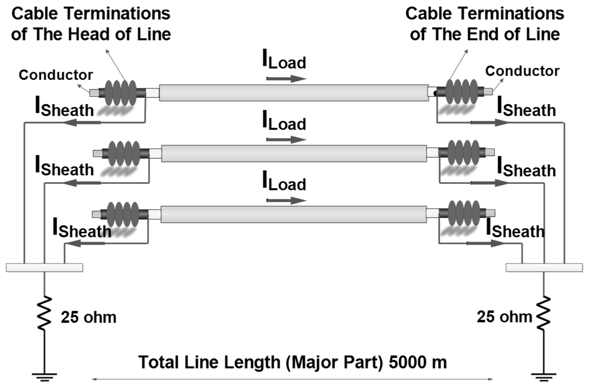
Processes 12 02909 g001
Figure 2. The cable configurations.
Processes 12 02909 g002
Figure 3. The zero sequence path in a high-voltage power cable line.
Processes 12 02909 g003
Figure 4. SSBLR method.
Processes 12 02909 g004
Figure 5. The Pareto front.
Processes 12 02909 g005
Figure 6. Hybrid ANN algorithm.
Processes 12 02909 g006
Figure 7. The input matrix for training.
Processes 12 02909 g007
Figure 8. The output matrices for training.
Processes 12 02909 g008
Figure 9. The input matrix for prediction.
Processes 12 02909 g009
Figure 10. The prediction process of MV in the optimum minor part detection algorithm.
Processes 12 02909 g010
Figure 11. The optimum minor part detection algorithm with the MV.
Processes 12 02909 g011
Figure 12. The Pareto front and Pareto points.
Processes 12 02909 g012
Figure 13. The new input matrix for the prediction of MC and MHC.
Processes 12 02909 g013
Figure 14. The prediction process for the MC of each Pareto point.
Processes 12 02909 g014
Figure 15. The prediction process for the MHC of each Pareto point.
Processes 12 02909 g015
Figure 16. Solid bonding.
Processes 12 02909 g016
Figure 17. The Pareto front and the Pareto points for Case 1.
Processes 12 02909 g017
Figure 18. The Pareto front and the Pareto points for Case 2.
Processes 12 02909 g018
Figure 19. The Pareto front and the Pareto points for Case 3.
Processes 12 02909 g019
Figure 20. The Pareto front and the Pareto points for Case 4.
Processes 12 02909 g020
Figure 21. The Pareto front and the Pareto points for Case 5.
Processes 12 02909 g021
Figure 22. The Pareto front and the Pareto points for Case 6.
Processes 12 02909 g022
Figure 23. The Pareto front and the Pareto points for Case 7.
Processes 12 02909 g023
Figure 24. The Pareto front and the Pareto points for Case 8.
Processes 12 02909 g024
Figure 25. The Pareto front and the Pareto points for Case 9.
Processes 12 02909 g025
Table 1. SC and the cable temperature.
SC (A)010203040
CT (°C)43.154.474.2119.0184.1
Table 2. Current, voltage and harmonic distortion rates of a high-voltage line.
Line Current (A)Line Voltage (kV)THDI (%)THDV (%)
L148524.73.974.20
L248524.75.445.30
L345524.73.183.04
Table 3. Comparison of grounding methods.
The Bonding MethodThe Sheath Current The Sheath VoltageHarmonic Distortion
Single point bondingnot taken into accountabove touch voltage limitnot taken into account
Solid bondingtaken into accountunder touch voltage limitnot taken into account
Cross Bondingtaken into accountabove touch voltage limitnot taken into account
SSBLRtaken into accountunder touch voltage limittaken into account
Table 4. The results of the solid bonding method.
The Head of Line Cable Terminations ValuesThe End of Line Cable Terminations Values
ParametersPhasesPhases
L1L2L3L1L2L3
MV (V)798822647786793630
MC (A)181179173176175169
MHC (%)5.874.753.475.895.013.45
Table 5. The optimum minor part parameter values of the dominant Pareto points on the Pareto front for Case 1.
PointL (m)Rg1 (ohm)Rg2 (ohm)Lg1 (H)Lg2 (H)
A19812.4990.00860.0014
B2012240.00840.0051
C18423.16190.00730.0048
D188623.290.00710.0059
E20912.24.210.003250.0014
F2042540.00430.0038
G20210120.00580.0051
H18311190.00810.0082
Table 6. The optimum minor part parameter values of the dominant Pareto points on the Pareto front for Case 2.
PointL (m)Rg1 (ohm)Rg2 (ohm)Lg1 (H)Lg2 (H)
A23411.89.660.00920.0062
B2247.321.660.00990.0078
C24313.4623.080.00910.0071
D21814.463.270.00880.00751
Table 7. The optimum minor part parameter values of the dominant Pareto points on the Pareto front for Case 3.
LabelL (m)Rg1 (ohm)Rg2 (ohm)Lg1 (H)Lg2(H)
A20121.518.480.00880.0029
B20611.773.730.0070.0026
C20218.7115.360.00820.0052
D20111.3312.290.00830.0057
E2074.3110.030.00590.0039
F18214.819.230.0110.0102
G20014.1812.180.00350.0018
Table 8. The optimum minor part parameter values of the dominant Pareto points on the Pareto front for Case 4.
PointL (m)Rg1 (ohm)Rg2 (ohm)Lg1 (H)Lg2 (H)
A1947.259.310.00590.0096
B2117.94120.00860.0055
Table 9. The optimum minor part parameter values of dominant the Pareto points on the Pareto front for Case 5.
PointL (m)Rg1 (ohm)Rg2 (ohm)Lg1 (H)Lg2 (H)
A2133.5513.360.00720.0095
B21913.623.280.00480.0096
Table 10. The optimum minor part parameter values of the dominant Pareto points on the Pareto front for Case 6.
LabelL (m)Rg1 (ohm)Rg2 (ohm)Lg1 (H)Lg2 (H)
A21110.6410.100.00730.0067
B2076.4312.390.00460.0070
C2026.492.750.00440.0016
Table 11. The optimum minor part parameter values of the dominant Pareto points on the Pareto front for Case 7.
PointL (m)Rg1 (ohm)Rg2 (ohm)Lg1 (H)Lg2 (H)
A2042.1095917.658970.009040.00720
B20610.68774140.009360.00816
C20821.674389.7632490.001130.00708
Table 12. The optimum minor part parameter values of dominant Pareto points on the Pareto front for Case 8.
PointL (m)Rg1 (ohm)Rg2 (ohm)Lg1 (H)Lg2 (H)
A21214.778.630.00510.0033
B21923.0116.030.00630.0072
C22617.055.140.00150.0084
D23624.2113.370.00950.0025
E24921.906.230.00860.0030
Table 13. The optimum minor part parameter values of the dominant Pareto points on the Pareto front for Case 9.
PointL (m)Rg1 (ohm)Rg2 (ohm)Lg1 (H)Lg2 (H)
A1755.1214.200.00930.0095
B1859.8010.850.00550.0038
C1899.7910.850.00540.0040
D19114.2911.470.00390.0057
E19214.1011.430.00400.0058
F19111.448.170.00590.0073
Table 14. The simulation results for the Pareto front solution in Case 1.
ValuesABCDEFGH
HLELHLELHLELHLELHLELHLELHLELHLEL
MV1 (V)91166842594055487432585143403640
MV2 (V)96187344634357527934625345423842
MV3 (V)77105436493048365926444533292928
MC1 (A)33332525252624256969414122231414
MC2 (A)32322424242523246667394021221313
MC3 (A)30302323242423236363383820211313
MHC1 (%)2.802.872.822.902.882.952.812.892.702.732.772.822.502.612.512.97
MHCI2 (%)3.543.573.463.503.403.443.453.503.843.853.603.633.633.693.463.55
MHCI3 (%)5.275.315.275.335.295.345.235.295.455.475.275.305.015.084.985.08
Table 15. The simulation results for the Pareto front solution in Case 2.
ValuesABCD
HLELHLELHLELHLEL
MV1 (V)7452745973596556
MV2 (V)7956806376656959
MV3 (V)6242585162475048
MC1 (A)2526232425252323
MC2 (A)2425222224242222
MC3 (A)2324212223242121
MHC1 (%)2.852.942.802.892.812.912.782.87
MHC2 (%)3.423.483.403.473.453.503.393.45
MHC3 (%)5.385.445.245.325.235.305.155.22
Table 16. The simulation results for the Pareto front solution in Case 3.
ValuesABCDEFG
HLELHLELHLELHLELHLELHLELHLEL
MV1 (V)81288030 66446445664552495127
MV2 (V)8631853270476849695055535429
MV3 (V)6821662555355436573442413919
MC1 (A)2929363625262424353515154344
MC2 (A)2828343424252323333412144242
MC3 (A)2727333323242223323314143939
MHC1 (%)2.812.892.792.852.812.892.812.902.782.842.822.942.462.52
MHC2 (%)3.503.543.553.593.463.513.453.503.543.583.443.423.883.91
MHC3 (%)5.275.325.285.325.245.305.275.335.275.315.205.295.065.10
Table 17. The simulation results for the Pareto front solution in Case 4.
ValuesAB
HLELHLEL
MV1 (V)40666946
MV2 (V)42717250
MV3 (V)32555936
MC1 (A) 21212526
MC2 (A)20202424
MC3 (A)202023224
MHC1 (%)2.82.892.802.88
MHC2 (%)3.413.463.433.48
MHC3 (%)5.235.305.225.28
Table 18. The simulation results for the Pareto front solution in Case 5.
ValuesAB
HLELHLEL
MV149684180
MV251744484
MV342532870
MC122222526
MC220212424
MC320202324
MHC12.802.892.752.84
MHC23.413.463.413.46
MHC35.245.315.145.20
Table 19. The simulation results for the Pareto front solution in Case 6.
ValuesABD
HLELHLELHLEL
MV1 (V)595644687728
MV2 (V)626047738230
MV3 (V)484637556323
MC1 (A)252529305454
MC2 (A)242428285252
MC3 (A) 232427275050
MHC1 (%)2.792.872.792.862.732.77
MHC2 (%)3.433.483.493.523.713.73
MHC3 (%)5.215.275.255.305.305.33
Table 20. The simulation results for the Pareto front solution in Case 7.
ValuesABC
HLELHLELHLEL
MV1 (V)454044421794
MV2 (V)464343471999
MV3 (V)38253233783
MC1 (A)151614144142
MC2 (A)151513134040
MC3 (A)141412133838
MHC1 (%)2.502.672.502.673.062.16
MHC2 (%)3.533.623.443.553.773.81
MHC3 (%)5.015.114.985.094.524.58
Table 21. The simulation results for the Pareto front solution in Case 8.
ValuesABCDE
HLELHLELHLELHLELHLEL
MV1 (V)513455642110199279935
MV2 (V)54365968231061063010538
MV3 (V)3826445498984218029
MC1 (A)20302727373833333636
MC2 (A)29292626363631323434
MC3 (A)27272525343530303333
MHC1 (%)2.502.582.072.162.752.812.802.882.792.86
MHC2 (%)3.713.763.623.693.553.583.513.553.553.59
MHC3 (%)5.005.064.414.515.275.325.225.285.275.32
Table 22. The simulation results for the Pareto front solution in Case 9.
ValuesABCDEF
HLELHLELHLELHLELHLELHLEL
MV1 (V)475058424334314742624758
MV2 (V)495562454536334945654962
MV3 (V)403949333424223631523449
MC1 (A)161633332425242433332425
MC2 (A)151531322320232331312324
MC3 (A)151531312222222230302323
MHC1 (%)2.87.22.82.82.52.52.52.62.82.82.82.9
MHC2 (%)3.35.33.53.53.63.53.63.73.53.53.43.5
MHC3 (%)5.25.85.25.35.05.05.05.15.35.35.25.3
Table 23. The dominant Pareto points in each of the cases.
The Case DPP PM-OML (m)Rg1 (ohm)Rg2 (ohm)Lg1 (H)Lg2 (H)
The Case 1HENN, GA18311190.00810.0082
The Case 2DENN, PSO21814.463.270.00880.00751
The Case 3FENN, GSA18214.819.230.0110.0102
The Case 6AMGR, GSA21110.6410.100.00730.0067
The Case 7BH-GA, GA20610.68774140.009360.00816
The Case 8BH-GA, PSO21923.0116.030.00630.0072
The Case 9AH-GA, GSA1755.1214.200.00930.0095
Table 24. The simulation results for the dominant Pareto points.
ValuesENN, GAENN, PSOENN, GSAMGR, GSAH-GA, GAH-GA, PSOH-GA, GSA
HLELHLELHLELHLELHLELHLELHLEL
MV1 (V)3640655652495956444255644750
MV2 (V)3842695955536260434759684955
MV3 (V)2928504842414846323344544039
MC1 (A)1414232315152525141427271616
MC2 (A)1313222212142424131326261515
MC3 (A)1313212114142324121325251515
MHC1 (%)2.512.972.782.872.822.942.792.872.502.672.072.162.817.17
MHC2 (%)3.463.553.393.453.443.423.433.483.443.553.623.693.375.30
MHC3 (%)4.985.085.155.225.205.295.215.274.985.094.414.515.225.83
Disclaimer/Publisher’s Note: The statements, opinions and data contained in all publications are solely those of the individual author(s) and contributor(s) and not of MDPI and/or the editor(s). MDPI and/or the editor(s) disclaim responsibility for any injury to people or property resulting from any ideas, methods, instructions or products referred to in the content.

