Forecasting CO₂ Emissions in India: A Time Series Analysis Using ARIMA

Abstract

This study evaluates the capability of the ARIMA (Auto Regressive Integrated Moving Average) to predict CO₂ emissions in India using data from 1990 to 2023, addressing a critical need for accurate forecasting amid various economic and environmental uncertainties. It is observed that ARIMA yields high accuracy with respect to the prediction, and hence, it is reliable for environmental forecasting. These predictions give policymakers evidence-based information to aid in implementing sustainable climate policies within India. To ensure reliable predictions, the study methodology utilizes the Box–Jenkins approach, which encompasses model identification, estimation, and diagnostic checking. The initial step in the study is the Augmented Dickey–Fuller (ADF) test, which assesses data stationarity as a prerequisite for precise time series forecasting. Model selection is guided by the Akaike Information Criterion (AIC), which balances prediction accuracy with model complexity. The efficiency of the ARIMA model is assessed by comparing the actual observed values to the predicted CO₂ emissions and the results demonstrate ARIMA’s effectiveness in forecasting India’s CO₂ emissions, validated by statistical measures that confirm the model’s robustness. The value of the present study lies in its focused assessment of the relevance of the ARIMA model to the specific environmental and economic context of India, with actionable insight for policymakers. This study enhances prior research by incorporating a focused approach to data-driven policy formulation that increases climate resilience. The establishment of a reliable model for the forecasting of CO₂ will aspire to support informed decision making in environmental policy and help India move forward toward sustainable climate goals. This study only serves to highlight the applicability of ARIMA in terms of environment-based forecasting and permits further emphasis on how much this method can be a useful data-based tool in climate planning.

1. Introduction

The increasing environmental and economic challenges associated with climate change underscore the importance of robust predictive models to assess and mitigate its impact. Predicting CO₂ emissions is essential for comprehending the course of climate change and for developing strategies for sustainable development. Making successful environmental plans requires precise forecasting, especially considering India’s increasing emission levels, which are a significant contribution to global greenhouse gas emissions [1,2,3]. The ARIMA (Auto Regressive Integrated Moving Average) model is one of the advanced time series forecasting techniques used in this study to examine the trends in India’s CO₂ emissions. This study attempts to offer insightful information that will help policymakers navigate the many problems of climate action by analyzing historical trends in India’s emissions [4]. Comprehending the variations, enduring patterns, and possible seasonality in CO₂ emissions might enable interested parties to make informed choices for sustainable growth [5,6,7].

The continuously increasing rate of CO₂ emission is highly threatening the global climatic condition and affecting almost every section of the world. According to Raihan et al. (2022), addressing the challenges of these areas with respect to a reduction in CO₂ emission and increasing environmental quality has made it a crucial priority at the global level towards the attainment of sustainable growth and mitigation of adverse climatic conditions [8]. India is an emerging and developing country that happens to be the seventh most vulnerable to climate change according to the Global Climate Risk Index 2020 [9]. For a better contrast, India is among the fastest-growing economies of the world. The World Bank adds that fast economic and population growth highly relies on fossil fuels, providing about 74% of the energy needs for India [10]. The unprecedented increase in this energy source and economic growth has therefore caused a massive increase in the country’s CO₂ emissions. In being the third largest emitter of carbon in the world, the country contributed 7% of the world’s emissions in 2020. CO₂ emissions in the country increased by 4.8% in 2018, the increase equally distributed within the power sector, transport and other industries [11]. The high consumption of fossil fuel and ever-increasing energy demand have brought severe environmental and ecological consequences to India, threatening its sustainable development goals. It raises critical questions about whether economic growth is combined with improved environmental sustainability.

Precise CO₂ forecasting plays a pivotal role in aiding policymakers to identify high-priority sectors requiring immediate emission reductions, optimize resource allocation, and track progress toward achieving sustainable development goals. Such forecasting equips decision-makers with actionable insights, enabling targeted interventions to mitigate climate impacts effectively. For environmental stakeholders, it offers a data-driven foundation to monitor progress, advocate for stringent climate policies, and ensure accountability in meeting global climate commitments. Given India’s significant contribution to global emissions, its CO₂ trajectory directly influences global climate dynamics. Successful emission reductions in India can substantially enhance international efforts to combat climate change and limit global warming.

Because it offers insights into patterns and trends throughout time, time series data analysis is extensively useful across disciplines like meteorology, epidemiology, finance, and environmental research. To predict CO₂ emissions in India, we use fundamental time series concepts such as stationarity, ACF, partial autocorrelation function (PACF), and the ARIMA model. A key component of time series data is stationarity, which is the ability of a series to maintain its statistical characteristics across time, including mean, variance, and autocorrelation. In the absence of trends or seasonality, ensuring stationarity makes modelling easier and produces more accurate forecasts [12].

The classical machine learning methods have developed the ability to learn complex patterns in data, which involves minimal human interference [13]. Classic machine learning models have been widely utilized for the forecast of CO₂ emissions, in which the most general techniques include linear regression analysis [14,15], support vector machines [16], random forest [17], neural network autoregressive model [14] and feed-forward neural networks [18]. However, a very important bottleneck for these machine learning techniques regarding CO₂ forecasting is that, unlike statistical methods for time series analysis, these machine learning techniques are not inherently capable of dealing with time series. First, machine learning models consider all the data points to be independent and identically distributed, whereas in the case of a time series, the observations will be highly related and have temporal dependencies. Another important aspect is that time-series data often contain an underlying trend and seasonal variation, hard to capture with classic machine learning algorithms without serious preprocessing [19].

Emission reduction and environmental quality are considered global priorities in relation to sustainable growth, fighting against the dangers of climatic change. This research contributes to investigating the impact of economic growth, renewable energy use, urbanization, industrialization, tourism, agricultural productivity, and forest area on CO₂ emissions in India between 1990 and 2020 using the Dynamic Ordinary Least Squares method [9].

In fact, all other statistical time series methods are designed to work with datasets that are sequential in nature—like for the recordings of CO₂ measurement consistently over time. Methods such as autoregressive, moving average, exponential smoothing, and structural models are all naturally suited to handle this sequential data structure. Among these methods, the ARIMA model has emerged as one of the most applied for CO₂ emissions forecasts [18].

Among the many approaches used in the literature on time series analysis and environmental forecasting is the ARIMA model, which is well known for its convenience of use and effectiveness in identifying linear patterns in time series data. Testing for stationarity with visual evaluations, the Augmented Dickey–Fuller (ADF) test, and the Kwiatkowski–Phillips–Schmidt–Shin (KPSS) test are crucial prior to implementing time series models. These tests establish if there is a regular, predictable trend in the time series across the examined period [20,21].

ACF gives these correlations a visual representation, while autocorrelation quantifies the link between a time series and its lagged values. Seasonality may be suggested by a sharp drop in autocorrelation at a certain lag, while non-stationarity is shown by a gradual decay. On the other hand, when calculating the correlation between a data point and its lagged values, the PACF plot separates the impact of intermediate lags, which is very useful for figuring out the sequence of an autoregressive process.

One of the most used methods for time series forecasting is the ARIMA model, which consists of three primary parts: Moving Average (MA), Integrated (I), and Auto-Regressive (AR). Features of the time series are captured by each component [1,22,23,24,25]:

Auto-Regressive (AR): The link between the current observation and its historical values is captured by auto-regressive (AR) analysis. The AR component’s order, represented by “p”, indicates how many lags were considered.

Integrated (I): The term “integrated” (I) describes the process of differencing time series data to attain stationarity. The “d”, which stands for differencing order, denotes how frequently differencing is used.

Moving Average (MA): Takes into consideration the effect of previous white noise or random shocks. “q”, the order of the MA component, indicates how many lag forecast mistakes are incorporated into the model.

The AIC, a frequently used metric in model selection, evaluates the level of fitness of a statistical model while taking complexity into account. The AIC value is very helpful in ARIMA modelling since it helps balance the trade-off between model complexity and performance. Better-fitting models with fewer parameters are shown by lower AIC values, which provide an objective means of comparing different parameter combinations (p, d, and q) and choosing the best model for precise forecasting. As a result, AIC is a crucial tool for determining the best ARIMA model for CO₂ emissions forecasting that balances predictability and simplicity [26,27].

The current work of research on time series analysis in environmental science is expanded by using ARIMA to forecast CO₂ emissions in India. To build models that account for long-term trends and possible seasonality, this study makes use of historical data on CO₂ emissions from India. Since it can offer insights that direct the creation of policies and the distribution of resources in attempts to slow down climate change, accurate emissions data forecasting is essential. This method is in line with earlier studies on emissions forecasting, which show how important historical data analysis is for strategic planning and environmental management (Figure 1) [1].

The main tool for this study’s methodological implementation is R software (RStudio 2024.09.0). R, which is well known for its statistical computing and data processing skills, provides the adaptability and transparency needed to create and assess intricate forecasting models like ARIMA. India’s environmental policies and sustainable development goals can be supported by data-driven decision making, made possible by R’s vast library of statistical tools, which enable accurate forecasting [28,29].

Because it uses differencing to handle nonstationary data, the ARIMA model is very useful for time series forecasting. This makes it appropriate for environmental datasets, which frequently show trends because of ongoing shifts in industrialization, energy use, and human activities. Although ARIMA has demonstrated potential in emissions forecasting, research has pointed out that it is not very good at taking sudden shocks or abrupt changes in environmental data into account. Nevertheless, ARIMA can provide competitive accuracy for short- to medium-term emissions forecasting with the right parameter tweaking.

For predicting complex, nonlinear interactions in environmental data, machine learning approaches have recently gained popularity as alternatives to conventional statistical models. ARIMA, being simpler and consuming fewer computational resources, is theoretically well suited and outcompetes LSTM on handling small datasets and time series with a linear trend. Furthermore, ARIMA does not require extensive training or tuning, in contrast to LSTM, and hence, it remains far more accessible and efficient for simple stationary series analyses [30].

ARIMA models can be used for a variety of emissions forecasting scenarios. Research has extended the use of ARIMA to several contaminants and environmental indicators in several different industries. One study, for example, used ARIMA to anticipate urban PM_2.5 and PM₁₀ pollution levels. This showed that ARIMA was useful for creating baseline projections, but further modelling was needed to take abrupt changes in environmental regulations or industrial operations into consideration. For similar applications in agricultural emissions, where seasonal patterns are prominent, weather-related factors had to be added to improve the accuracy of the model [31,32,33].

The aim of this study is to provide the fundamental ideas of time series analysis for environmental forecasting, such as the significance of stationarity and the functions of ARIMA, PACF, and ACF in emissions data prediction. By using these techniques, scientists and environmental analysts can learn about the trends in CO₂ emissions over time, which helps them make well-informed decisions on things like sustainability planning and climate policy.

2. Methodology

2.1. Data Preparation

Data Cleaning and Preprocessing: Missing values or outliers are checked in the data, which contain values. To preserve the quality of the data, all variations are handled carefully.

2.2. Stationarity Testing Using ADF

Stationarity Check: Since stationarity suggests that the data’s statistical characteristics (such mean and variance) remain constant over time, it is a crucial prerequisite for time series modelling using ARIMA. For the model to correctly detect and forecast recurring patterns in the data, trends or seasonality must be eliminated for CO₂ emissions in India. The ARIMA model may produce skewed or unstable forecasts if the series is non-stationary because it may mistakenly interpret trends as continuous patterns. By ensuring that the model concentrates on the actual underlying relationships, stationarity produces forecasts that are more accurate and dependable. The detection of unit roots, which signify non-stationarity in the data, is performed using the Augmented Dickey–Fuller (ADF) test [34].

Differencing for Stationarity: Differencing is used if it is determined that the data are not stationary. This involves lowering the emissions value from the prior year from the emissions value from the current year. The results of the ADF test and a visual examination of the time series plot are used to calculate the necessary degree of differencing. For example, if it stabilizes the mean and enables a more accurate ARIMA model, a first-order difference (i.e., one level of differencing) would be adequate.

2.3. ACF and PACF Analysis for Model Identification

Autocorrelation and Partial Autocorrelation: ACF gives these correlations a visual representation, while autocorrelation quantifies the link between a time series and its lagged values. Seasonality may be suggested by a sharp drop in autocorrelation at a certain lag, while non-stationarity is shown by a gradual decay. On the other hand, when calculating the correlation between a data point and its lagged values, the PACF plot separates the impact of intermediate lags, which is very useful for figuring out the sequence of an autoregressive process. When choosing the right model parameters for ARIMA modelling, ACF and PACF charts offer crucial insights into the structure of time series data.

Plots of the ACF and PACF are essential instruments for figuring out the sequence of the ARIMA model’s elements. While the PACF plot aids in separating the direct impacts of each lag, the ACF plot shows correlations between the series and its lagged values [35].

Order Selection: We can determine possible orders for the autoregressive (AR) and moving average (MA) components by looking at graphs. Significant spikes in the ACF plot at lags, for instance, would point to an MA component, whereas spikes in the PACF plot might point to an AR component. The choice of the (p, d, q) parameters in ARIMA is guided by this analysis, where:

• p is the order of the AR term;
• d is the number of differencing required to make the series stationary;
• q is the order of the MA term.

2.4. Model Selection Using AIC

AIC Calculation and Model Evaluation: The AIC is used to assess various model configurations following the identification of possible orders for the ARIMA model. By penalizing extra parameters, the AIC reduces the chance of overfitting and helps strike a balance between the model’s complexity and goodness of fit.

Optimal Model Selection: The model that best fits the data is the one with the lowest AIC score. This model should ensure accurate projections without needless complexity by offering a reasonable balance between accuracy and simplicity. CO₂ emissions forecasts for the future are based on the chosen ARIMA model [36].

2.5. Forecasting CO₂ Emissions

Generating Forecasts: After determining the best ARIMA model, we create projections for CO₂ emissions. The output of the model provides a range of expected future emissions, including both point projections and confidence ranges. This stage offers useful forecasts that help direct environmental regulations.

Validation and Comparison: By contrasting the predicted emissions with actual emissions data (when values become available), the accuracy of the model is assessed. This comparison enables us to evaluate the prediction ability of the model and, if required, modify it for upcoming projections. If the Mean Absolute Percentage Error (MAPE) value is approximately close to 10, then it indicates high model accuracy. For instance, extra variables like economic indicators or policy changes may need to be considered if the predicted value deviates greatly from the observed values [37].

3. Result and Analysis

Understanding Emission Trends: The final study reveals underlying trends in CO₂ emissions throughout time in addition to forecasts. Context for the projections is provided by discussing insights into the growth rate, stability, and any notable changes in emission levels.

Implications for Policy: This study intends to assist decision-makers in developing environmental policy by precisely forecasting future emissions. The findings can be used to track India’s progress toward its emission reduction goals and predict future difficulties in limiting CO₂ emissions.

3.1. Stationarity Testing Using the ADF Test

The Augmented Dickey–Fuller (ADF) test was used to ascertain whether the CO₂ emissions data are stationary. The ADF test’s null hypothesis (H₀) suggests that there may be a unit root, which would suggest non-stationarity. A p-value of 0.01 and a Dickey–Fuller test statistic of −4.4891 were obtained from the ADF test. We reject the null hypothesis, since the p-value is less than the significance level of 0.05, which shows that the CO₂ emissions data are stable. This is a crucial discovery since stationarity keeps trends from skewing the data, guaranteeing the accuracy of ARIMA-based forecasting.

A differencing value of d = 2 was selected based on the dataset, as the first series showed significant non-stationarity, most likely because of a clear trend. Persistent patterns in the ACF and PACF plots and the stationarity test demonstrated that the series still showed evidence of non-stationarity after applying initial differencing (d = 1). However, the dataset reached stationarity, with the mean and variance stabilizing and no significant trends remaining after applying second differencing (d = 2). To convert the data into a stable series suited for ARIMA modelling, d = 2 is appropriate, as demonstrated by the ACF plot, which shows no significant autocorrelations at higher lags, and the PACF plot, which only identifies significant correlations at the first few lags.

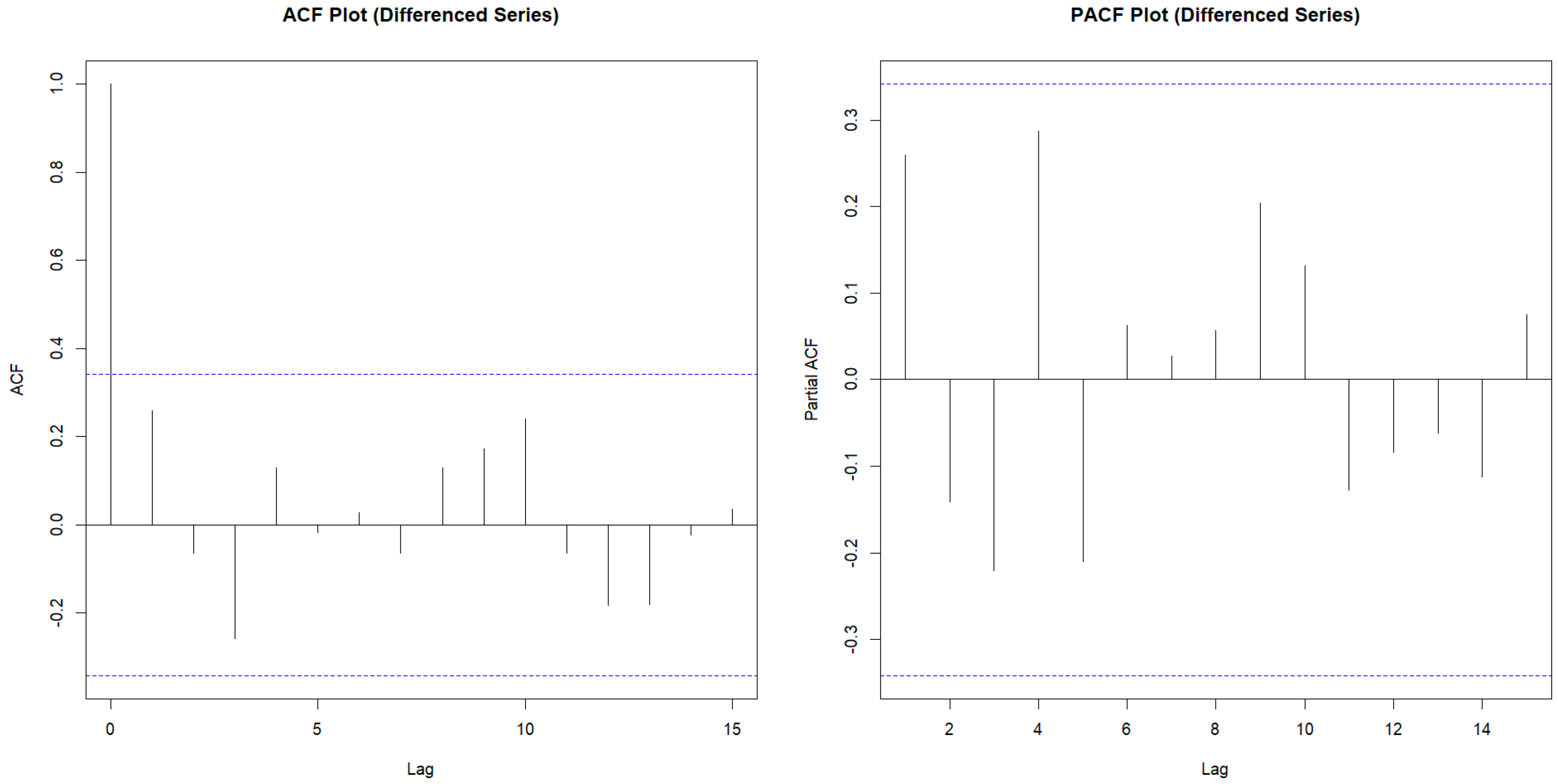
3.2. ACF and PACF Analysis for Model Identification

We examined the ACF and PACF plots following the procedure of second-order differencing (d = 2) to determine the proper values of p (autoregressive order) and q (moving average order) for the ARIMA model. The selection of the AR and MA components is aided by these graphs, which show any connections or dependencies in the data.

3.3. ACF Analysis

With autocorrelation values near zero at all lags, the ACF plot for the differenced series showed no notable spikes. This implies that there are no notable autocorrelations in the data, and therefore, an autoregressive component is not helpful. Because of this, we set the autoregressive order p to 0, which means that, in the context of this dataset, past values of the time series have little predictive value for current values.

3.4. PACF Analysis

On the other hand, lag 4 displayed a significant spike in the PACF plot, whereas the remaining lags were quite modest and lacked significant associations. This spike at lag 4 indicates that the data have a substantial moving average relationship, meaning that the last four years’ worth of random shocks or error terms can accurately estimate the current value of CO₂ emissions. The moving average order q is thus set to 4.

Figure 2 below shows the plot for ACF and PACF.

3.5. ARIMA Model Selection

There were no notable lags in the ACF plot, and all autocorrelation values stayed within the confidence intervals. The absence of notable spikes suggests that there is no need for a moving average (MA) component because the series’ current values do not exhibit a strong correlation with lagged values. To simplify the model and make sure it accurately depicts the underlying structure of the data, the moving average order p was set to 0. On the other hand, no significant correlations were found at any of the other lags, and the PACF plot showed a clear spike at lag 4. After taking into consideration the impacts of intermediate lags, this single spike suggests that there is a significant correlation between the series’ present value and its value four steps earlier. The addition of a fourth-order autoregressive component (q = 4) to the model is supported by this finding.

ARIMA (0, 2, 4) is the most suitable model structure for the CO₂ emissions data, according to the ACF and PACF plot evaluations. This model setup consists of the following:

p = 0: The absence of significant autocorrelation in the ACF plot indicates that there is no autoregressive component (p = 0).

d = 2: The Augmented Dickey–Fuller test verified that stationarity was achieved using second-order differencing.

q = 4: A moving average component of the fourth order derived from the PACF plot’s spike.

Based on ACF and PACF analysis, which indicates strong autocorrelations at higher lags and the requirement for two differencing steps to ensure stationarity, ARIMA (0, 2, 4) was chosen to model CO₂ emissions in India. Additionally, the model minimizes the AIC, suggesting that fitness and complexity are well balanced. But it is important to prevent overfitting, which can happen if the model becomes too complicated and captures both the underlying pattern and noise, making it difficult to generalize to fresh data. ARIMA (0, 2, 4) achieves a balance between a strong fit to historical data and preserving generalizability for future predictions by employing a very simple model with few AR components and maximizing the MA terms.

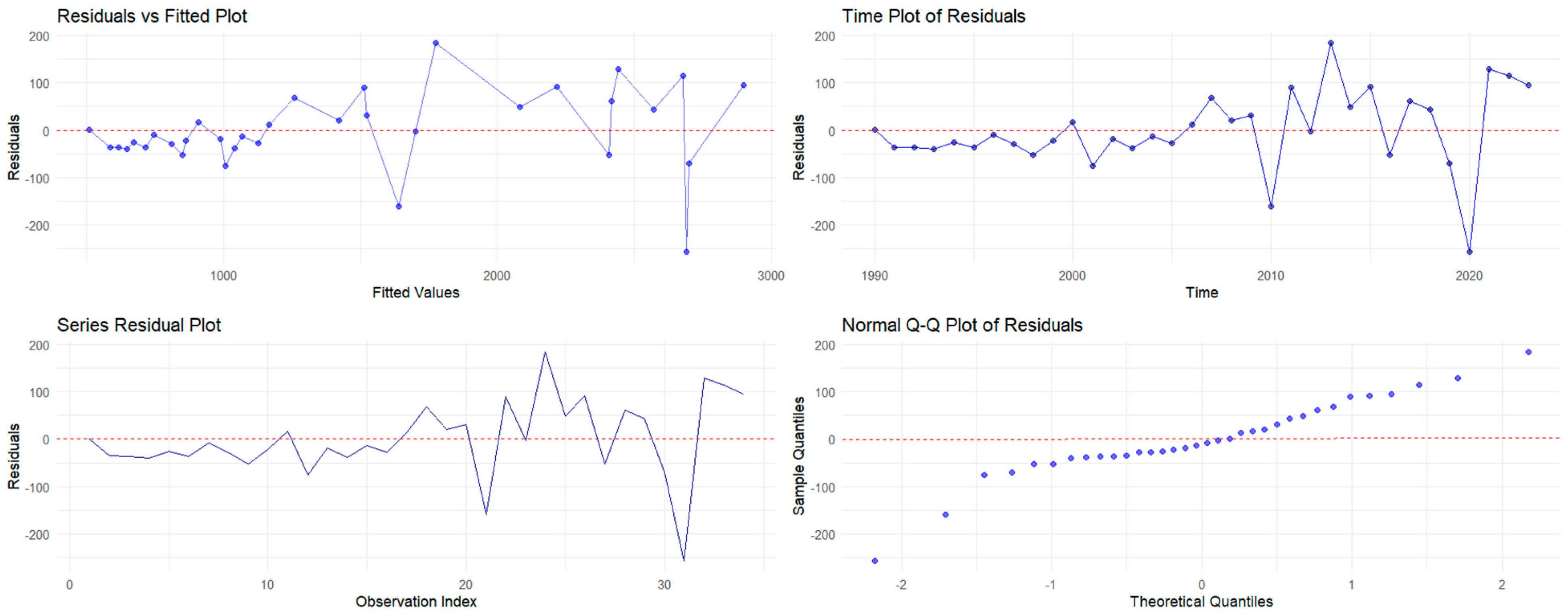
3.6. Residual Analysis

We carried out an in-depth residual study to guarantee the ARIMA (0, 2, 4) model’s dependability. To verify that the residuals, which are the variations between the model’s fitted values and the observed values, complied with the presumptions of the ARIMA framework, they were analyzed, as shown in Figure 3.

Fitted Values against Residuals Plot: There were no obvious patterns or trends in the plot of residuals against fitted values, suggesting that the ARIMA model successfully represented the structure of the data. Random distribution close to zero indicated that no significant explanatory information was left unmodeled and that the model effectively captured all detectable information in the data. The absence of residual trends demonstrates that the model was not subjected to structural bias or underfitting.

Residuals Time Series Plot: The residuals moved wildly about zero, with no obvious periodic patterns or systematic shifts over time, according to the time series plot. This residual variation’s randomness demonstrated that the model’s proper differencing and order selection had adequately removed autocorrelations from the original series.

ACF Plot: The residuals’ unpredictability was further confirmed by the ACF plot. The idea that the residuals resembled white noise was supported by the fact that no discernible autocorrelation was seen at any latency. This suggests that there is no residual structure to explain because the ARIMA (0, 2, 4) model accurately captured all pertinent information from historical data.

Normal Q-Q Plot of Residuals: The Q-Q plot showed that the points mainly lined up along the reference line, indicating that the residuals were normally distributed. In real-world applications, small tail variations are to be expected, but they have little effect on the model’s dependability. Forecasts and confidence intervals from the model are guaranteed to be statistically valid and understandable due to the residuals’ normality.

Collectively, the diagnostic evaluation verified the ARIMA (0, 2, 4) model’s robustness and efficiency. The model avoided overfitting and maintained simplicity while producing accurate forecasts by attaining unpredictability and white noise behavior in residuals. The residual analysis also shows that the model accurately depicts the dynamics of India’s historical CO₂ emissions.

The chosen ARIMA (0, 2, 4) model, which was determined to be the best match based on its AIC value, has been used to create forecasts for the year 2021–2023. These projections go beyond the documented trends in historical data to offer expected CO₂ emission amounts in 2021–2023. Based on historical data, the ARIMA model accurately predicts probable future patterns in CO₂ emissions.

Table 1. Comparison between actual and forecasted CO₂ emissions.

Year	Actual	Forecasted	Accuracy
2021	2571.40	2988.94	83.76
2022	2794.83	3066.43	90.28
2023	2994.79	3179.42	93.83

compares the projected CO₂ emissions for 2021–2023 with the actual observed emissions to assess the predictive accuracy of the ARIMA (0, 2, 4) model. In an 80:20 ratio, the data are divided into a training set and a test set. The degree to which the model’s predictions match the actual CO₂ emissions is evaluated in this examination. The model appears to be successful in identifying underlying trends in CO₂ emissions, as evidenced by the excellent connection between expected and actual values. On the other hand, notable disparities could indicate areas for possible enhancement or different modelling approaches and expose constraints in the model’s predictive power.

The discrepancies between predicted and actual CO₂ emissions are shown in Figure 4. Some projections show significant differences from actual values, while others closely match them. These discrepancies are explained by the intrinsic difficulties of predicting environmental data, which are impacted by a wide range of uncontrollable variables. This comparative study is essential for verifying the forecasting model’s accuracy and boosting trust in its capacity to anticipate future CO₂ emissions.

Using the well-known ARIMA (0, 2, 4) model, forecasts for the years 2024–38 involve estimating CO₂ emissions for each upcoming year. The model utilizes patterns and trends identified in historical data during the analysis to generate these estimates. By extending existing trends, the ARIMA model aims to provide insights into future CO₂ emission levels, helping to inform environmental policy and strategic planning.

From the plotted time series forecast, the following is clearly shown in Figure 5:

Rising Trend: The predicted values exhibit a distinct rising trend, indicating a steady increase in CO₂ emissions. This pattern is consistent with past data as well as the anticipated expansion of India’s GDP and energy usage.

Increasing Rate: As the projected period draws to a close, the rate of increase appears to be quickening, suggesting a possible spike in emissions in the years to follow.

This study provides a comprehensive interpretation of the ARIMA model’s output and forecast trends for CO₂ emissions in India. The time series analysis effectively highlights key patterns and future projections. Comparing the observed trends to underlying economic or policy issues is crucial, nevertheless, to deepen the research. For example, times of urbanization, industrial expansion, or rising energy consumption brought on by economic growth may all be associated with higher CO₂ emissions. On the other hand, any reductions or slower rise in emissions that are seen could be related to the adoption of clean energy laws, advances in technology, or global agreements like the Paris Agreement. An analysis that ties these findings to economic or policy developments in India, like the encouragement of renewable energy sources or more strict environmental laws, would give a more insightful and defined understanding of the trends and provide important information about the factors influencing India’s trajectory of CO₂ emissions.

3.7. Error Metrics

Kumari and Singh (2023), observed that ARIMA’s predicted values are too far from the actual CO₂ emissions. The authors used ARIMA (1, 2, 1) for prediction. It can be seen that the ARIMA model has a MAPE value of 98.969%, which is inaccurate. Therefore, the authors conclude that forecasting for 2020 to 2030 will not be appropriate [38].

In this paper, the model successfully captures the underlying trends with acceptable errors, as evidenced by the Root Mean Square Error (RMSE) value of 306.69, which is a reasonable degree of accuracy for CO₂ emissions forecasting. The model’s dependability is demonstrated by the Mean Absolute Error (MAE) value of 291.25, which indicates high predictive performance because the average error is small in relation to the amount of CO₂ emissions. The Mean Absolute Percentage Error (MAPE) value is approximately near 10, which indicates high model accuracy, as shown in

Table 2. Error metrics for CO₂ emission.

Error Metrics	ARIMA
RMSE	306.69
MAE	291.25
MAPE	10.71%

.

4. Discussion

Using an ARIMA (0, 2, 4) model, the time series projection for CO₂ emissions in India shows a worrying rising trend. According to this model’s particular specifications, the previous four error terms have an impact on the current emissions value. Furthermore, to obtain stationarity, the necessary condition for efficient time series analysis, the data require second-order differencing.

A mix of industrial and socioeconomic variables are responsible for the reported increase in CO₂ emissions in India. The dependence on fossil fuels like coal and petroleum, which are major contributors to greenhouse gas emissions, has grown dramatically because of rapid industrialization. Population growth and urbanization have increased the requirement for energy for residential, transportation, and electrical purposes. The expansion of India’s economy has also led to a rise in energy-intensive industries like manufacturing and construction. Also, because renewable energy technologies like solar and wind have not been widely adopted, the nation’s energy mix still significantly favors non-renewable sources. The issue is made worse by inefficient policies, such as those that postpone the implementation of clean energy transitions or the enforcement of pollution restrictions. Another significant industry, agriculture, indirectly contributes through methane emissions, and the increasing number of cars raises CO₂ levels through transportation-related emissions. The persistent rise in CO₂ emissions is caused by these coupled variables, which calls for extensive action measures to slow the trend.

These elements are probably going to have a long-term impact on emissions levels as India develops more. The forecast line’s shaded confidence interval illustrates the inherent unpredictability of future projections. Numerous factors, such as shifts in legislation, technical breakthroughs, and economic swings, contribute to this unpredictability. The degree of uncertainty rises as we go farther into the future, according to a broader confidence interval toward the end of the prediction period [39,40,41].

Several assumptions need to be considered when using time series analysis to predict CO₂ emissions in India over the long run (2024–2038). First, the model assumes that historical trends, patterns, and connections in the data will persist in the future, which might not take into consideration prospective structural shifts in the economy, advances in technology, or changes in policy. One of the main causes of CO₂ emissions is economic activity, which includes increases in energy use, transportation, and industrial production. Future economic developments, such as a move toward more environmentally friendly sectors of the economy or modifications to the way people use energy, could, nevertheless, drastically modify the emissions trajectory.

This forecast is important and has broad significance. Rising sea levels, harsh weather, and biodiversity loss are just a few of the environmental effects of climate change and global warming brought on by rising CO₂ emissions. Furthermore, rising CO₂ emissions have the potential to worsen air pollution, which would be detrimental to people’s health and welfare. Implementing strong climate policies and regulations, encouraging the use of renewable energy sources, promoting energy efficiency, and fostering international collaboration are all essential to lessening these effects.

However, it is critical to recognize the ARIMA model’s shortcomings. In practical situations, the model’s assumptions of stationarity, linearity, and constant variance might not always hold true. Furthermore, emissions trends can be greatly impacted by unforeseen external variables like technological advancements or geopolitical events. To adjust to changing conditions, it is crucial to continuously monitor CO₂ emissions and update the forecast on a frequent basis.

It is essential to concentrate on industries and transportation that contribute the most to CO₂ emissions to improve recommendations. For example, increasing the infrastructure for electric vehicles (EVs), encouraging public transit, or implementing more stringent fuel efficiency regulations could all help cut emissions in the transportation sector. Norway’s successful promotion of EVs through tax exemptions and subsidies has resulted in a significant reduction in transportation-related emissions. In the industrial sector, deploying energy-efficient technologies and shifting to greener fuels can cut emissions. Similar tactics could be used in India, as evidenced by Germany’s legislation encouraging the use of renewable energy in industrial operations, such as its Renewable Energy Sources Act. Policymakers can prioritize effective actions and make quantifiable progress in reducing emissions by customizing such sector-specific recommendations to India’s circumstances.

India needs to take a variety of approaches to addressing the issues brought on by growing CO₂ emissions. Strong climate rules and regulations must be put into place, renewable energy sources like solar, wind, and hydro power must be promoted, energy efficiency must be encouraged, and international collaboration must be fostered. To adjust to shifting conditions, it is also essential to regularly update the forecast and monitor CO₂ emissions continuously. India can strive toward a more sustainable future by being aware of the consequences of the CO₂ emission prediction and taking proactive steps. To lessen the negative consequences of climate change and guarantee a healthy planet for future generations, a coordinated effort involving the government, business community, and citizens is required [4].

While the ARIMA model has proved efficient in forecasting based on the given historical data, there are several drawbacks with this approach that may affect precision in the CO₂ emission forecasts. For example, sudden changes in trends such as government policies increasing stringency in emissions regulations or promotion of renewable energy technologies can easily result in abrupt changes in the trends. ARIMA cannot consider such external changes since it relies on pattern continuity from the past and hence can fail to give forecasts with accuracy. Of course, other challenges will be economic shocks, such as recession. This could temporarily lower the industrial activities and, in turn, reduce emissions, misleading ARIMA to think that a long-term decline has started. Likewise, with sudden economic growth, the emissions could shoot up, resulting in discrepancies in the forecast.

Technological changes, the sudden and widespread diffusion of renewable energy technologies or major successes in carbon capture can lead to nonlinear variations in the emissions trend, for which ARIMA is unprepared. For example, there was a reduction in global emissions due to COVID-19 because of reduced industrial activity; this was an unexpected event which ARIMA would not predict. This uncertainty increases with longer-term forecasts, as external factors such as geopolitical events and resource availability become more influential. Integration of ARIMA with machine learning models or hybrid approaches that incorporate nonlinear interactions and external factors can be carried out to improve reliability for more robust and dynamic predictions.

Limitation and Future Scope

Although a strong tool, the ARIMA model has drawbacks that may affect how accurately CO₂ emissions are predicted. Among these restrictions are the presumptions of linearity, stationarity, and outlier sensitivity. Furthermore, the model can have trouble capturing intricate patterns and nonlinear interactions. While linearity suggests that the correlations between present and historical values are linear, stationarity argues that the time series’ statistical characteristics, such as mean and variance, stay constant over time. These assumptions might not hold true in real-world situations because of things like structural breaks, seasonal effects, or outside shocks that affect the data [42].

Unexpected economic events, such as a recession, global pandemic, or rapid adoption of renewable energy, disrupt normal historical patterns in emissions and make ARIMA’s forecasts inefficient. Sometimes, during an economic decline, industrial activities decrease, which is usually accompanied by a reduction in energy use, temporarily reducing CO₂ emissions. Only given information about historical patterns, ARIMA might overgeneralize and become overly pessimistic once the economy has recovered. Analogously, the rapid growth of renewable energy or the sudden changes in technology abruptly alter the trend of emissions, which ARIMA models cannot grasp; hence, it also faces limitation for such dynamic and nonlinear scenarios.

The prediction power of the model can be increased by incorporating external elements like economic data, climate legislation, and technological improvements. By combining several models, ensemble approaches can lessen the influence of the biases and uncertainties of individual models. To deal with non-stationarity, techniques like seasonal decomposition or transformations (such as log or power transformations) could be used. Similarly, by identifying nonlinear relationships or dynamic patterns in the data, other models like ARIMA-GARCH or machine learning techniques like LSTMs could enhance ARIMA. Prior knowledge and uncertainty can be included in the forecasting process using Bayesian approaches. Finally, data-driven strategies like machine learning can assist in locating intricate links and patterns in the data, producing projections that are more accurate [43,44,45].

Different policy measures are suggested as effective in containing CO₂ emissions. Taxes related to high-ecological-impact activities should be expensive, carbon taxes should be levied, and cap-and-trade systems, together with carbon offsets and environmental technology standards, will steer pro-sustenance behaviors. Initiatives on educating the public about sources of pollution and the resultant environmental impacts are much needed. The facilitation of free public transit and promotion of electric vehicles can reduce national fuel consumption, resulting in lower carbon footprints. There are opportunities to diversify into low-carbon energy technologies, such as carbon-free hydrogen and low-carbon biofuels. Gradually, the dependency on coal will be reduced, evolving a leading position in renewable energy. Furthermore, industrial emissions abatement by a voluntary approach must be pursued [45].

The forecast of CO₂ emission in this study is univariate and does not consider exogenous factors that might emanate from population growth, economic development and/or technological change, along with shifts to renewable energy sources, and even government policies that are likely to evolve in the future. Such a future study could also develop more comprehensive, multifactorial models for emission forecasting, which will be useful for policymakers by giving them a fuller picture.

5. Conclusions

A disturbing increasing trend is revealed by the study of the time series forecast for CO₂ emissions in India, which was produced using an ARIMA (0, 2, 4) model. The main forces behind this development are industrialization, rising energy use, and economic expansion. Although the model offers insightful information, it also draws attention to the inherent uncertainties in future projections. The trajectory of emissions can be greatly impacted by variables such as changes in legislation, technical breakthroughs, and economic swings. This prediction has wide-ranging effects. Increasing CO₂ emissions cause climate change and global warming, which have several negative effects on the ecosystem. Furthermore, rising CO₂ emissions have the potential to worsen air pollution, which would be detrimental to people’s health and welfare. Implementing strong climate policies and regulations, encouraging the use of renewable energy sources, promoting energy efficiency, and fostering international collaboration are all essential to lessening these effects.

The analysis emphasizes the significance of using data-driven policymaking to address CO₂ emissions. Important quantitative findings, including anticipated emission levels by 2038, indicate the pressing need for efficient actions. Prioritizing emissions reduction in high-impact industries and transportation, encouraging the use of renewable energy sources, and implementing stronger environmental laws are examples of concrete actions. Additionally, as variables like policy changes, economic shifts, and technology breakthroughs evolve, projections stay accurate and pertinent thanks to adaptive forecasting, which updates models with fresh data on a regular basis. This ongoing monitoring strategy strengthens India’s commitment to addressing climate change by allowing policymakers to assess progress toward emission objectives and make appropriate adjustments.

Increased sea levels, biodiversity loss, and extreme weather events that endanger ecosystems and livelihoods are just a few of the dire effects of unchecked CO₂ emissions, which worsen climate change. The financial consequences, such as skyrocketing catastrophe recovery costs and medical bills linked to pollution, further emphasize how urgently sustainable emission control measures are needed to protect the environment and the general welfare.

Nonetheless, it is critical to recognize the ARIMA model’s limitations. In practical situations, the model’s assumptions of stationarity, linearity, and constant variance might not always hold true. Furthermore, emissions trends can be greatly impacted by unforeseen external variables like technological advancements or geopolitical events. To adjust to changing conditions, it is crucial to continuously monitor CO₂ emissions and update the forecast on a frequent basis. India can strive toward a more sustainable future by being aware of the consequences of the CO₂ emission prediction and taking proactive steps. To lessen the negative consequences of climate change and guarantee a healthy planet for future generations, a coordinated effort involving the government, business community, and citizens is required.