Aggregation Modeling for Integrated Energy Systems Based on Chance-Constrained Optimization

Abstract

Integrated energy systems (IESs) strengthen electricity–gas–heat multi-energy coupling and reduce wind and light abandonment. For grids with superior distribution, IESs are similar to virtual energy storage systems and are able to realize efficient interaction with the grid by synergizing the operating status of the internal equipment and improving the security, economy, and flexibility of the grid’s operation. However, the internal equipment coupling of an IES is complex, and determining how to evaluate its adjustable capacity range (that is, the upper and lower boundaries of its external energy demand) considering the uncertainty and volatility of wind power and photovoltaic output is a problem to be solved. To solve this problem, this paper presents a chance-constrained evaluation method for the adjustable capacity of IESs. Firstly, mathematical models and operational constraints of each device within the IES are established. Secondly, based on the mathematical model of chance-constrained planning, an adjustable capacity range assessment model considering the uncertainty of wind and photovoltaic output is established. Finally, the MATLAB/Yalmip/Gurobi solver is used for the optimization solution, and the adjustable capacity range interval of the constructed IES model is solved using an arithmetic example to analyze and verify the correctness and validity of the method and to study the influencing factors of its adjustable range.

1. Introduction

With the growth of the economy and productivity, the demand for primary energy sources, such as coal and oil, is also increasing. However, the combustion of these sources and their secondary processed products produce large amounts of harmful greenhouse gases. Therefore, the development of renewable energy power generation, such as hydroelectricity, wind power, and photovoltaic power generation, and improvements in the rate of consumption of renewable energy have become widespread concerns for all countries in the world [1]. According to the World Energy Outlook 2019 published by the U.S. Energy Information Administration (EIA), between 2018 and 2050, the share of electricity generated from renewable sources will have increased from 18% to 31% [2]. However, renewable energy’s output is highly affected by weather, with uncertainty and volatility, which challenges the safe and stable operation of power systems. In order to consume more renewable energy and achieve the safe and stable operation of power systems, many scholars at home and abroad have proposed the concept of IESs.

Multi-energy coupling can effectively enhance energy utilization [3,4,5,6]. IESs are important types of user-side multi-energy coupling systems that can effectively solve energy shortage problems, enhance the utilization of renewable energy, and reduce the emissions of pollutant gases. They have gradually become an important development trend for future energy supply systems [7]. At present, many scholars have obtained many important results on the optimal scheduling of IESs. The authors of [8] proposed a two-stage scheduling energy management model with day-ahead and real-time scheduling, which effectively improves the economy of IES operation.

On the energy supply side, since the output of new energy is influenced by many factors, such as wind speed, light, and temperature, the uncertainty and stochasticity of its output cause certain difficulties in the optimal scheduling of IESs. Methods such as stochastic optimization [9] and robust optimization [10,11], along with others, can solve these sub-problems more effectively. The authors of [12] proposed an electrically coupled IES distribution-robust optimal scheduling model that considers wind power uncertainty, which is described using a fuzzy set constructed based on the confidence of the probability density function. The authors of [13] proposed a method based on an improved conditional value-at-risk (CVaR) to address the uncertainty of wind power and photovoltaic output and analyzed the P2G technique to improve the economic efficiency of the system to consume wind and PV power.

Due to the large amount of greenhouse gas emissions, carbon emissions have become an important issue to be considered in the operation of IESs [14,15,16]. The authors of [17] integrated multiple energy storage types including compressed air energy storage, batteries, and thermal storage into an IES, establishing a new type. The authors of [18] used carbon capture (CCU) to build a CO₂ emission model based on life-cycle theory and established an IES dispatch model based on life-cycle assessment and CCU, which can effectively reduce carbon emissions.

However, the above studies targeted the optimal operation scheduling of IESs, with objectives of operation cost minimization or revenue maximization. Under the background of coordination of power grids and flexible resources of loads, it is a promising method to provide regulation capacity of flexible resources from demand sides to promote the operation efficiency of power grids. As resources such as batteries are gradually allocated on the demand side and the complementarity of the multi-energy sector, the power interaction of an IES with power grids is no longer fixed. Hence, it is important for an IES’s participating grid-load coordination to accurately assess the IES’s regulation capability. In this aspect, ref. [19] proposed a sequential recursive method to assess the range of the adjustable capability of IESs under different initial states. Ref. [20] considered the demand response and economic constraint conditions, proposed an electrically coupled IES with an adjustable capacity range, and drew Pareto curves of its external electrical energy demand and natural gas demand under different scenarios. However, there are few studies investigating the regulation capacity of IESs considering multiple uncertainties.

In this context, in order to more accurately describe an IES’s adjustable capacity under the consideration of wind and PV output uncertainty, this paper proposes a chance-constrained, optimization-based adjustable capacity assessment method for IESs. The contributions are summarized as follows:

(1)

The mathematical model and operation constraints of multi-energy equipment are established. Based on this, the basic framework for the steady-state operation of IESs is constructed and an aggregation model is established to demonstrate the regulation capacity of the IES.

(2)

Uncertainties of distributed energy resources such as wind power and photovoltaic are involved in the proposed model to obtain a confidence assessment result. The chance constraints are developed to model these uncertainties, and then the proposed model with chance constraints is reformulated into a mixed-integer linear programming problem to reduce computational burdens.

(3)

Economic budgets are considered in the proposed model and a multi-objective optimization model is developed and solved to identify the regulation capacity of the IES.

The rest of this paper is organized as follows. The basic structure and model of the IES is given in Section 2. The economic constraints are formulated in Section 3. The assessment model and solving process are demonstrated in Section 4. Case studies are given to demonstrate the effectiveness and feasibility of the proposed model in Section 5, and this paper is concluded in Section 6.

2. The Basic Structure of an Integrated Electricity–Heat System and Its Model

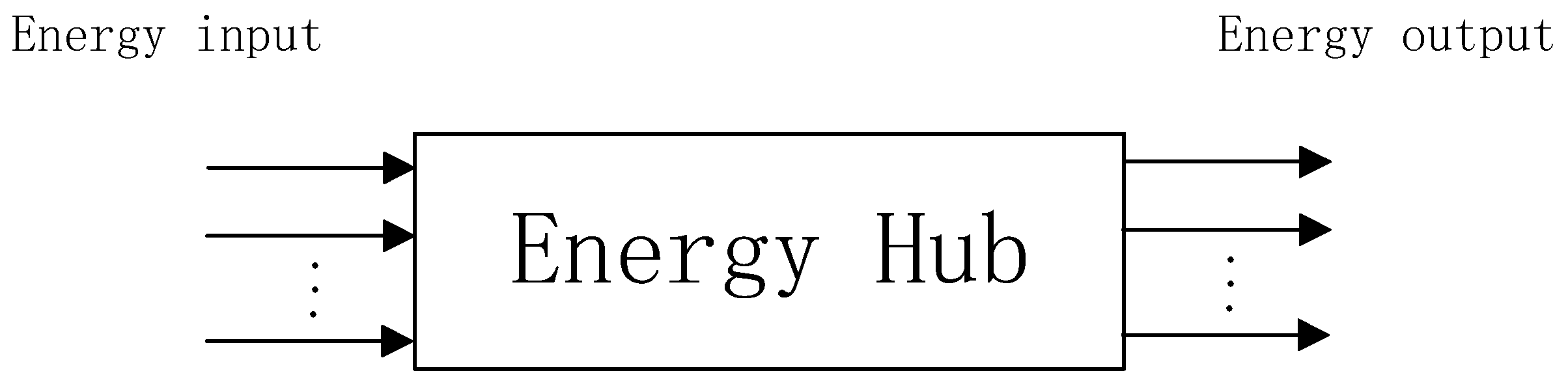
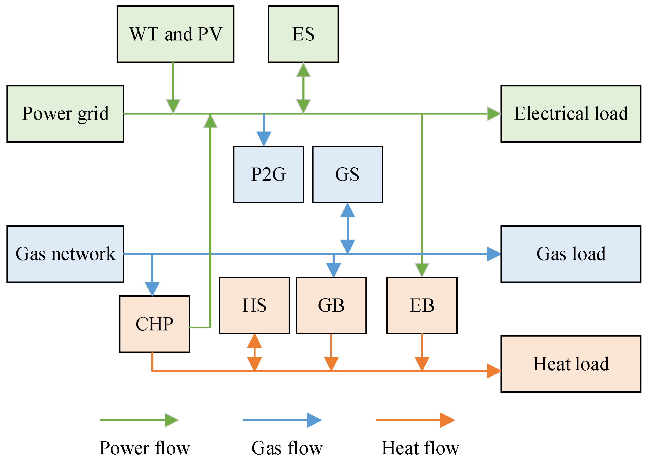
2.1. Basic Structure

IESs include the three following main bodies: an energy supply module, an energy coupling module, and an end user module. The energy coupling module, as the hub of energy transmission and transformation, obtains energy from the energy supply module, converts it into different energy forms, such as electricity, heat, and gas, through a variety of energy coupling devices, and then sells it to the end user module. The end user adjusts their demand for energy through demand response elasticity. This, in turn, affects the energy demand of the entire IES [21].

No matter how complex the energy coupling relationship in the IES is, various energy inputs are needed. They are ultimately converted into another form of energy as the output of the system, so an IES can be described as an input–output dual port network, as shown in Figure 1. The box in the middle of the figure is the IES analyzed in this work.

The comprehensive energy system structure built in this study is shown in Figure 2. Three kinds of energy are included—gas, heat, and electricity. In terms of equipment selection and planning, the system includes wind power (WT) and photovoltaic (PV) generator sets, power-to-gas equipment (P2G), combined heat and power (CHP) generation, a gas boiler (GB), and an electric boiler (EB). The energy storage device includes electricity storage (ES), gas storage (GS), and heat storage (HS). In the diagram, the green arrows represent the electrical energy flow in the IES, the blue arrows represent the natural air flow, and the orange arrows represent the thermal energy flow.

2.2. Modeling of IES

2.2.1. Energy Coupling Device

The energy coupling devices of the IES built in this study mainly include the following: (1) the EB includes two processes—heat storage and heat release, which convert electric energy into heat energy through water heating to supply the heat load. (2) The GB is able to convert natural gas’s chemical energy into heat energy by burning it to obtain hot water or high-temperature water steam and maintaining the balance between the supply and demand of the heat energy in the system. (3) By burning natural gas, the CHP can produce both electric energy and heat energy, making it one of the important energy conversion devices in the IES. (4) The additional electricity generated by wind power and PV power or unconsumed electricity can be converted by the P2G into synthetic natural gas for storage or consumed during peak load energy consumption. The P2G first produces O₂ and H₂ by electrolyzing water, and then combines the H₂ with CO₂ to produce CH₄ [22].

The mathematical models and operating constraints of the above coupled devices are as follows:

$$\left\{\begin{array}{l}{H}_{\mathrm{EB},t}={\eta }_{\mathrm{EB}}{P}_{\mathrm{EB},t}\\ 0\le P_{\mathrm{EB},t}\le P_{\mathrm{EBmax}}\\ H_{\mathrm{GB},t}=G_{\mathrm{GB},t}{\eta }_{\mathrm{GB}}\\ 0\le H_{\mathrm{GB},t}\le H_{\mathrm{GBmax}}\\ P_{\mathrm{CHP},\min }\le P_{\mathrm{CHP},t}\le P_{\mathrm{CHP},\max }\\ P_{\mathrm{CHP},t}={\mu }_{\mathrm{CHP},\mathrm{P}}{G}_{\mathrm{CHP},t}\\ H_{\mathrm{CHP},t}={\mu }_{\mathrm{CHP},\mathrm{H}}{G}_{\mathrm{CHP},t}\\ R_{\mathrm{CHP},\mathrm{down}}\le P_{\mathrm{CHP},\mathrm{t}}-P_{\mathrm{CHP},\mathrm{t}-1}\le R_{\mathrm{CHP},\mathrm{up}}\\ G_{\mathrm{P}2\mathrm{G},t}={\eta }_{\mathrm{P}2\mathrm{G}}{P}_{\mathrm{P}2\mathrm{G},t}\\ 0\le P_{\mathrm{P}2\mathrm{G},t}\le P_{\mathrm{P}2\mathrm{G},\max }\end{array}\right.$$

(1)

where $H_{\mathrm{EB},t}$ is the heat power of the EB at time t; ${\eta }_{\mathrm{EB}}$ is the heat production efficiency of the EB (kW); $P_{\mathrm{EB},t}$ and $P_{\mathrm{EB}\text{\_}\max }$ are the electric power consumed by the EB at time t and the maximum power consumed, respectively (kW); $H_{\mathrm{GB},t}$ and $G_{\mathrm{GB},t}$ are the heat power and natural gas consumption power of the gas boiler at time t, respectively (kW); ${\eta }_{\mathrm{GB}}$ is the heat production efficiency of the GB; $H_{\mathrm{GBmax}}$ is the maximum heat power of the GB (kW); $P_{\mathrm{CHP},t}$ and $H_{\mathrm{CHP},t}$ are the generating power and heating power of the CHP, respectively (kW); $P_{\mathrm{CHP},\max }$ and $P_{\mathrm{CHP},\min }$ are the maximum and minimum generating power values of the CHP under the pure condensation condition, respectively (kW); $G_{\mathrm{CHP},t}$ is the consumption of gas power of the CHP during time t (kW); ${\mu }_{\mathrm{CHP},\mathrm{P}}$ and ${\mu }_{\mathrm{CHP},\mathrm{H}}$ are the power generation efficiency and heat production efficiency of the CHP, respectively; $P_{\mathrm{CHP},\mathrm{t}}$ is the active power output of the CHP; $R_{\mathrm{CHP},\mathrm{down}}$ and $R_{\mathrm{CHP},\mathrm{up}}$ are the downhill and uphill rates of the CHP, respectively (kW); $G_{\mathrm{P}2\mathrm{G},t}$ and $P_{\mathrm{P}2\mathrm{G},t}$, respectively, represent the power converted from P2G into artificial natural gas and the electric power consumed during time t (kW); ${\eta }_{\mathrm{P}2\mathrm{G}}$ is the conversion efficiency of the P2G; and $P_{\mathrm{P}2\mathrm{G},\max }$ is the maximum electric power consumed by the power-to-gas technology (kW).

2.2.2. Energy Storage Device

The energy storage system can transfer the energy over time, store the surplus energy, and release it when the energy is insufficient, smoothing the fluctuations in wind power, improving the power quality of the system, and thus reducing wind abandonment. The energy storage model constructed in this study includes electric storage (ES), heat storage (HS), and gas storage (GS) devices. The operation principle and energy conversion relationships of the three kinds of energy storage devices with different energy forms are similar, so a model can be used to describe them. Here, the electric energy storage device is taken as an example to provide a general description of the three energy storage devices.

The mathematical model of the ES operating in the state of energy storage and discharge is as follows:

$$\left\{\begin{array}{l}{W}_{\mathrm{es},t}=W_{\mathrm{es},t-1}+P_{\mathrm{esc},t}{\gamma }_{\mathrm{c}}\Delta t\\ W_{\mathrm{es},t}=W_{\mathrm{es},t-1}-{\displaystyle \frac{P_{\mathrm{esd},t}}{{\gamma }_{\mathrm{d}}}}\Delta t\\ W_{\mathrm{es},\min }\le W_{\mathrm{es},t}\le W_{\mathrm{es},\max }\\ 0\le P_{\mathrm{esc},t}\le B_{\mathrm{c},t}{P}_{\mathrm{esc},\max }\\ 0\le P_{\mathrm{esd},t}\le B_{\mathrm{d},t}{P}_{\mathrm{esd},\max }\\ B_{\mathrm{c},t}+B_{\mathrm{d},t}\le 1\\ W_{\mathrm{es},0}=W_{\mathrm{es},T}\end{array}\right.$$

(2)

where $W_{\mathrm{es},t}$ is the storage capacity of the battery at time t (kWh); ${\gamma }_{\mathrm{c}}$ and ${\gamma }_{\mathrm{d}}$ are the charging efficiency and discharging efficiency of the battery, respectively; $P_{\mathrm{esc},t}$ and $P_{\mathrm{esd},t}$ are the charging power and discharging power of the battery at time t, respectively (kW); $W_{\mathrm{es},\max }$ and $W_{\mathrm{es},\min }$ are the maximum storage capacity and minimum storage capacity of the battery at time t, respectively (kWh); $P_{\mathrm{esc},\max }$ and $P_{\mathrm{esd},\max }$ are the maximum allowable charging and discharging power of the battery, respectively (kW); $B_{\mathrm{c},t}$ and $B_{\mathrm{d},t}$ are 0/1 variables, representing the two states of charge and discharge, respectively; and $W_{\mathrm{es},0}$ and $W_{\mathrm{es},\mathrm{T}}$ are the storage capacities at the beginning and end of the scheduling cycle, respectively (kWh).

2.3. Demand Response Model

The demand response (DR) means that users can adjust their electricity consumption according to incentive mechanisms or changes in the electricity price, interact with the grid, optimize the load curve, promote the consumption of renewable energy, and improve the operating efficiency of the system [23,24].

When considering the DR, the load types on the demand side can be divided into the following: (1) a rigid load is an uncontrollable and fixed load, and its power consumption time and mode do not change. (2) A shiftable load can adjust its power consumption time according to the plan, but it needs to shift its power consumption time as a whole. (3) A transferable load can flexibly change the consumption time and the power consumption at each moment, but in the entire scheduling cycle, the sum of the transferred load is 0; that is, the total load remains unchanged. (4) A reducible load can interrupt part of the running time or reduce the consumption according to the dispatching instruction or power plan, and it can partially or completely reduce its own load according to the specific situation.

The similarity between loads (2) and load (3) is that they can both adjust their power consumption according to the dispatching instructions. The difference is that when the DR of the shiftable load occurs, its power consumption time and power need to shift as a whole, the operation process cannot be suspended, and the consumption cannot be changed. When the transferable load has a demand response, the operation of part of the load can be interrupted, and the power and running time can be freely adjusted. Therefore, there is no need to shift the entire demand response, but the total amount of the load before and after the DR occurs cannot be changed. Its demand response features are more flexible than those of shiftable loads. Taking an electric load as an example, various loads were modeled and analyzed.

2.3.1. Shiftable Load

When the DR of a shiftable load occurs, its mathematical model and operation constraint are as follows:

$$\left\{\begin{array}{l}{\displaystyle \sum _{t=1}^T{\alpha }_t}=t_{\mathrm{con}}\\ {\displaystyle \sum _{t=t_{st}}^{t_{st}+t_{\mathrm{con}}-1}{\alpha }_t}\ge t_{\mathrm{con}}({\alpha }_t-{\alpha }_{t-1}-\dots -{\alpha }_{t-t_{\mathrm{con}}+1})\end{array}\right.$$

(3)

where ${\alpha }_t$ represents the translation state of the shiftable load at a certain time t; ${\alpha }_t=1$ indicates that the load shifts, ${\alpha }_t=0$ indicates that the load does not shift; $t_{\mathrm{st}}$ represents the start time; and $t_{\mathrm{con}}$ represents the continuous running time of the shiftable load.

2.3.2. Transferable Load

Users can transfer this load from the peak demand time of electricity consumption or the expensive electricity price to the low demand time or cheap electricity price. They can flexibly arrange the time for electricity consumption and transfer the load.

The constraints are as follows:

$$\left\{\begin{array}{l}-P_{\mathrm{tran},\min }\le P_{\mathrm{tran},t}\le P_{\mathrm{tran},\max }\\ {\displaystyle \sum _{t=1}^T{P}_{\mathrm{tran},t}=0}\end{array}\right.$$

(4)

where $P_{\mathrm{tran},\min }$ and $P_{\mathrm{tran},\max }$ represent the minimum and maximum of the transferable load power, respectively (kW).

2.3.3. Reducible Load

The reducible load can reduce the consumption of the user, directly, at the peak of power consumption. A sign indicates the reduction state of the reduced load within a certain period of time, indicating the situation of the reduced load or that it is not reduced. The constraints are as follows:

$$\left\{\begin{array}{l}{P}_{\mathrm{cut},t}=(1-{\epsilon }_t{\delta }_t)P_{\mathrm{cut},t}^{\prime }\\ {\displaystyle \sum _{t=1}^{24}{\delta }_t}\le N_{\max }\end{array}\right.$$

(5)

where ${\epsilon }_t$ is the load reduction factor under time t, ${\epsilon }_t\in (0,1)$; $P_{\mathrm{cut},t}^{\prime }$ is the power before the load can be reduced to participate in scheduling (kW); and $N_{\max }$ is the maximum number of reductions.

3. Economic Constraint Model

The superior power supply system can dynamically adjust the operation strategy of an IES through customized time-sharing tariffs, so that peak cutting and valley filling can be achieved. Meanwhile, in order to improve the ability of IESs to consume wind and photovoltaic power and to reduce CO₂ emissions, the economic costs generated in the operation process of IESs are constrained based on the DR, and the various kinds of losses generated by the IES in the process of operation are modeled and analyzed in the form of economic costs. These economic costs include income from the sale of the electricity, the cost of purchasing electricity and gas, the cost of wind and solar abandonment penalties, the cost of the depreciation of the energy storage equipment, the cost of compensation for the demand response, and the cost of CO₂ emission penalties, which are modeled as follows.

3.1. Energy Purchase Cost

The power purchase cost of IESs includes the costs of power purchase and gas purchase minus the profit of power sales, and the constraints of power purchase and power sales are similar to the constraints of the energy storage equipment. Power purchases and power sales cannot be carried out at the same time, and their power should be within a certain range. The constraints are as follows:

$$\left\{\begin{array}{l}{C}_{\mathrm{buy}}=C_{\mathrm{P}}+C_{\mathrm{G}}-C_{\mathrm{sell}}\\ C_{\mathrm{P}}={\displaystyle \sum _{t=1}^{24}{p}_{\mathrm{P},\mathrm{buy},t}{P}_{\mathrm{buy},t}}\\ C_{\mathrm{G}}={\displaystyle \sum _{t=1}^{24}{p}_{\mathrm{G},\mathrm{buy},t}{G}_{\mathrm{buy},t}}\\ C_{\mathrm{sell}}={\displaystyle \sum _{t=1}^{24}{p}_{\mathrm{sell},t}{P}_{\mathrm{sell},t}}\end{array}\right.$$

(6)

$$\left\{\begin{array}{l}0\le P_{\mathrm{buy},t}\le U_{\mathrm{buy},t}{P}_{\mathrm{net}\text{\_}\max }\\ 0\le P_{\mathrm{sell},t}\le U_{\mathrm{sell},t}{P}_{\mathrm{net}\text{\_}\max }\\ 0\le U_{\mathrm{buy},t}+U_{\mathrm{sell},t}\le 1\end{array}\right.$$

(7)

where $C_{\mathrm{buy}}$, $C_{\mathrm{P}}$, $C_{\mathrm{G}}$, and $C_{\mathrm{sell}}$ are the IES’s total energy purchase cost, power purchase cost, gas purchase cost, and profit from selling power to the superior distribution network, respectively (CNY); $p_{\mathrm{P},\mathrm{buy},t}$, $p_{\mathrm{G},\mathrm{buy},t}$, and $p_{\mathrm{sell},t}$ are the power purchase, gas purchase rate, and power sale price, respectively (CNY/kW); and $U_{\mathrm{buy},t}$ and $U_{\mathrm{sell},t}$ identify the states of the power purchase and power sale, where $U_{\mathrm{buy},t}=1$ indicates that power is being purchased from the superior power network, and $U_{\mathrm{sell},t}=1$ indicates that the IES is selling electricity to the upper power grid.

3.2. Penalty Costs for Wind and Solar Abandonment

Because renewable energy cannot be fully consumed, the resulting abandonment of wind power and photovoltaic is penalized with a certain cost, as follows:

$$C_{\mathrm{d}}={\alpha }_{\mathrm{w}}{\displaystyle \sum _{t=1}^{24}(P_{\mathrm{w},t}-P_{\mathrm{wc},t})}+{\alpha }_{\mathrm{pv}}{\displaystyle \sum _{t=1}^{24}(P_{\mathrm{pv},t}-P_{\mathrm{pvc},t})}$$

(8)

where $C_{\mathrm{d}}$ is the cost of abandoning wind and solar (CNY); ${\alpha }_{\mathrm{w}}$ and ${\alpha }_{\mathrm{pv}}$ are the cost coefficients of abandoning wind and photovoltaic power, respectively; $P_{\mathrm{w},t}$ and $P_{\mathrm{pv},t}$ are the predicted wind power and photovoltaic power during time t, respectively (kW); and $P_{\mathrm{wc},t}$ and $P_{\mathrm{pvc},t}$ are the actual wind power and photovoltaic power consumed during time t, respectively (kW).

3.3. Depreciation Cost of Energy Storage Equipment

In this study, the built IES included an ES device, a GS device, and an HS device. Taking the ES device as an example, the mathematical model for its depreciation cost was established. The mathematical models for the depreciation costs of the GS device and HS device can be similarly established, as follows:

$$C_{\mathrm{sto}}={\displaystyle \sum _{t=1}^{24}(k_{\mathrm{esc}}{P}_{\mathrm{esc},t}+}{k}_{\mathrm{esd}}{P}_{\mathrm{esd},t})$$

(9)

where $C_{\mathrm{sto}}$ is the depreciation cost of the energy storage device (CNY); $k_{\mathrm{esc}}$ is the cost of storing unit power when the energy storage device is working in the energy storage state; and $k_{\mathrm{esd}}$ is the cost of releasing unit power when the ES device is working in the energy discharge state (CNY/kW).

3.4. Demand Response Compensates for Costs

Since the incentive demand response (IDR) load changes its energy use behavior according to the incentive mechanism, that is, according to the instructions issued by the superior power grid, the superior power grid will provide certain compensation, so there are compensation costs. The incentive demand response load considered in this study included electrical load and thermal load. The compensation costs are as follows:

$$\left\{\begin{array}{l}{C}_{\mathrm{DR}}=C_{\mathrm{shift}}+C_{\mathrm{tran}}+C_{\mathrm{cut}}\\ C_{\mathrm{shift}}=k_{\mathrm{shift}}{\displaystyle \sum _{t=t_{\mathrm{s}-}}^{t_{\mathrm{s}+}-t_{\mathrm{con}}+1}{P}_{\mathrm{shift},t}}\\ C_{\mathrm{tran}}=k_{\mathrm{tran}}{\displaystyle \sum _{t=t_{\mathrm{t}-}}^{t_{\mathrm{t}+}}{P}_{\mathrm{tran},t}}\\ C_{\mathrm{cut}}=k_{\mathrm{cut}}{\displaystyle \sum _{t=1}^{24}(P_{\mathrm{cut},t}^{\prime }-P_{\mathrm{cut},t})}\end{array}\right.$$

(10)

where $C_{\mathrm{DR}}$ is the total cost of the demand response, and $C_{\mathrm{shift}}$, $C_{\mathrm{tran}}$, and $C_{\mathrm{cut}}$ are the economic costs generated by the shifting load, the transferable load, and the reducible load, respectively (CNY); $k_{\mathrm{shift}}$, $k_{\mathrm{tran}}$, and $k_{\mathrm{cut}}$ are the compensation costs of the shifting unit power, the transferable unit power, and the reducing unit power, respectively (CNY/kW); and $P_{\mathrm{shift},t}$, $P_{\mathrm{tran},t}$, $P_{\mathrm{cut},t}^{\prime }$, and $P_{\mathrm{cut},t}$ are the power of the shifting load, the power of the transferable load, and the load power before and after reduction during time t, respectively, (kW).

3.5. Carbon Penalty Costs

At present, the electrical power industry allocates the initial carbon emission quota for free. If the CO₂ emissions generated during the actual operation process are higher than the initial carbon emission quota, a carbon emission cost will be generated. In this study, the carbon price of cascade trading was adopted. The higher the amount of carbon emissions generated, the higher the costs are of the carbon emission purchasing rights, and correspondingly, the greater the cost of the carbon emissions generated. The specific carbon emission cost calculation model is as follows:

$$E_{\mathrm{all}}={\displaystyle \sum _{t=1}^{24}(E_{\mathrm{Pgrid},t}+E_{\mathrm{Ggrid},t}-E_{\mathrm{P}2\mathrm{G},t})}-E_{\mathrm{IES}}$$

(11)

$$C_{\mathrm{car}}=\left\{\begin{array}{ll}\mu E_{\mathrm{all}}& E_{\mathrm{all}}\le l\\ \mu (1+\alpha )(E_{\mathrm{all}}-l)+\mu l& l\le E_{\mathrm{all}}\le 2l\\ \mu (1+2\alpha )(E_{\mathrm{all}}-2l)+\mu (2+\alpha )l& 2l\le E_{\mathrm{all}}\le 3l\\ \mu (1+3\alpha )(E_{\mathrm{all}}-3l)+\mu (3+3\alpha )l& 3l\le E_{\mathrm{all}}\le 4l\\ \mu (1+4\alpha )(E_{\mathrm{all}}-4l)+\mu (4+6\alpha )l& E_{\mathrm{all}}\ge 4l\end{array}\right.$$

(12)

$$\left\{\begin{array}{l}{E}_{\mathrm{Pgrid},t}={\mu }_{\mathrm{e}}{P}_{\mathrm{grid},t}\\ E_{\mathrm{Ggrid},t}={\mu }_{\mathrm{g}}{G}_{\mathrm{grid},t}\\ C_{\mathrm{P}2\mathrm{G},t}={\mu }_{\mathrm{P}2\mathrm{G}}{G}_{\mathrm{P}2\mathrm{G},t}\end{array}\right.$$

(13)

where $C_{\mathrm{car}}$ is the cost of carbon emissions (CNY); $\xi$ is the expense per unit of carbon emissions (m³/CNY); $l$ is the length of the carbon emission interval (m³); $E_{\mathrm{all}}$ represents the total CO₂ emissions (m³); $E_{\mathrm{Pgrid},t}$ and $E_{\mathrm{Ggrid},t}$ are the carbon emissions generated by the power purchase and gas purchase during time t, respectively (m³); $E_{\mathrm{P}2\mathrm{G},t}$ represents the CO₂ emissions absorbed by the P2G during time t (m³); $E_{\mathrm{IES}}$ is the free carbon emission credit of the IES (m³); ${\mu }_{\mathrm{e}}$ and ${\mu }_{\mathrm{g}}$ are the CO₂ emission factors of the power purchase and gas purchase, respectively (m³/kW); and ${\mu }_{\mathrm{P}2\mathrm{G}}$ is the carbon absorption factor of the P2G (m³/kW).

The total cost is as follows:

$$C_{\mathrm{total}}=C_{\mathrm{buy}}+C_{\mathrm{w}}+C_{\mathrm{pv}}+C_{\mathrm{sto}}+C_{\mathrm{car}}+C_{\mathrm{DR}}$$

(14)

4. Assessment Model of Adjustable Capability Based on Chance-Constrained Optimization

In this study the prediction of wind power and photovoltaic output is the input parameter in the proposed model. The output predictions of wind power and photovoltaic can be obtained by statistical or machine learning-based methods. However, all prediction methods would cause prediction errors, which would affect the accurate assessment of an IES’s adjustable capacity. This uncertainty should be fully considered when evaluating the adjustable range of an IES. Therefore, in this study, we established an IES adjustable capacity evaluation model based on the chance-constrained optimization theory that considers the uncertainty of wind power and photovoltaic output.

4.1. Chance-Constrained Optimization

As the outputs of wind power and PV are easily affected by weather factors, they have uncertainty and volatility. The chance constraints were introduced to model uncertainties of wind power and photovoltaic and the proposed model was transformed into a deterministic one to establish an evaluation model of the adjustable capacity range of the integrated energy system based on chance constraints. Finally, MATLAB 2021b software was used to apply the Gurobi 11.0 solver.

The mathematical model for chance-constrained planning is as follows:

$$\left\{\begin{array}{l}\min Ef(x,\zeta )\\ s.t.P_r\left\{g_i(x,\zeta )\le 0,i=1,2,\cdots ,d\right\}\ge {\beta }_i\\ x\in D\end{array}\right.$$

(15)

where $Ef(x,\zeta )$ is the expected value of the objective function given the decision and random variables; $x$ represents the decision variables; $\zeta$ represents the random variables; $P_r\left\{•\right\}$ is the probability of event $\left\{•\right\}$ occurring; $g_i(x,\zeta )\le 0$ represents the inequality constraints in the system; ${\beta }_i$ is the confidence level specifying the probability of a large event, ${\beta }_i\in (0,1)$; and $D$ is the set of deterministic constraints.

4.2. IES Adjustable Capacity Assessment Model

4.2.1. Constraint

The normal operation of the IES needs to satisfy the operational constraints of various energy devices, as shown in Equations (1)–(5), and the electric, gas, and thermal power balance conditions, as shown in Equations (16)–(18):

$$P_{\mathrm{grid},t}+P_{\mathrm{PV},t,\mathrm{c}}+P_{\mathrm{w},t,\mathrm{c}}+P_{\mathrm{esd},t}+P_{\mathrm{CHP},t}=P_{\mathrm{P}2\mathrm{G},t}+P_{\mathrm{esc},t}+P_{\mathrm{EB},t}+P_{\mathrm{load},t}$$

(16)

$$G_{\mathrm{grid},t}+G_{\mathrm{P}2\mathrm{G},t}+G_{\mathrm{gd},t}=G_{\mathrm{CHP},t}+G_{\mathrm{GB},t}+G_{\mathrm{gc},t}+G_{\mathrm{load},t}$$

(17)

$$H_{\mathrm{eb},t}+H_{\mathrm{rd},t}+H_{\mathrm{GB},t}+H_{\mathrm{CHP},t}=H_{\mathrm{rc},t}+H_{\mathrm{load},t}$$

(18)

where $P_{\mathrm{load},t}$, $G_{\mathrm{load},t}$, and $H_{\mathrm{load},t}$ are the electrical, gas, and thermal loads on the customer side, respectively, after considering the demand response. The economic cost constraints should also be satisfied.

$$C_{\mathrm{total}}\le C$$

(19)

The electric power balance constraint excluding the uncertainty of the wind power output is shown in Equation (16), considering prediction error on the wind power output. At the same time, in order to maintain the balance of the system’s electric power, errors are introduced into the wind power and PV power outputs. The above electric power balance constraint is changed to the following:

$$P_{\mathrm{grid},t}+(P_{\mathrm{PV},t,\mathrm{c}}+{\delta }_{\mathrm{pv},t})+(P_{\mathrm{w},t,\mathrm{c}}+{\delta }_{\mathrm{w},t})+P_{\mathrm{esd},t}+P_{\mathrm{CHP},t}=P_{\mathrm{P}2\mathrm{G},t}+P_{\mathrm{esc},t}+P_{\mathrm{EB},t}+P_{\mathrm{load},t}$$

(20)

where ${\delta }_{\mathrm{w},t}$ and ${\delta }_{\mathrm{pv},t}$ denote the errors in the predicted values of the wind and PV output power at time t, respectively.

The theory of chance-constrained planning was applied to establish Equation (20) with a confidence level no less than $\theta$. Thus, the electric power balance constraint of Equation (20) can be transformed as follows:

$$\mathrm{Pr}\{P_{\mathrm{grid},t}+(P_{\mathrm{PV},t,\mathrm{c}}+{\delta }_{\mathrm{pv},t})+(P_{\mathrm{w},t,\mathrm{c}}+{\delta }_{\mathrm{w},t})+P_{\mathrm{esd},t}+P_{\mathrm{CHP},t}\ge P_{\mathrm{P}2\mathrm{G},t}+P_{\mathrm{esc},t}+P_{\mathrm{EB},t}+P_{\mathrm{load},t}\}\ge \theta$$

(21)

Since the above equation contains random variables and cannot be solved directly, it is transformed into a deterministic constraint:

$$P_{\mathrm{grid},t}+P_{\mathrm{PV},t,\mathrm{c}}+P_{\mathrm{w},t,\mathrm{c}}+P_{\mathrm{esd},t}+P_{\mathrm{CHP},t}+F^{-1}(\alpha )\sqrt{{\sigma }_{\mathrm{PV},t}^2+{\sigma }_{\mathrm{w},t}^2}\ge P_{\mathrm{P}2\mathrm{G},t}+P_{\mathrm{esc},t}+P_{\mathrm{EB},t}+P_{\mathrm{load},t}$$

(22)

where $F^{-1}()$ denotes the inverse cumulative distribution function of the variable satisfying the normal distribution; and ${\sigma }_{\mathrm{w},t}^2$ and ${\sigma }_{\mathrm{PV},t}^2$ denote the variances in the normal distributions satisfied by the wind and PV power, respectively.

4.2.2. Objective

The adjustable capacity of the IES refers to its ability to regulate the power interacting with the superior grid, including the upper and lower limits of the interacting electrical energy power and the cumulative interacting power within each single time period, subject to satisfying the constraints of the system, as shown in Equation (23).

$$\left\{\begin{array}{l}\min P_{\mathrm{grid},t}\le P_{\mathrm{grid},t}\le \max P_{\mathrm{grid},t}\\ \min E_{\mathrm{grid},t}\le {\displaystyle \sum _{\tau =0}^t{P}_{\mathrm{grid},t}}\le \max E_{\mathrm{grid},t}\end{array}\right.$$

(23)

where $P_{\mathrm{grid},t}$ denotes the power interaction between the IES and the superior grid at moment t (kW); and $E_{\mathrm{grid},t}$ denotes the cumulative power interaction between the IES and the superior grid up to moment t (kWh).

Based on the chance-constrained planning theory, the following four adjustable-capacity assessment models were built separately, and the Gurobi solver was used to optimize the solution to comprehensively describe the adjustable capacity range of the IES. Since the models used to solve the lower boundary (min) and upper boundary (max) problems were different in the constructed models, they needed to be studied separately.

$$\begin{array}{l}\min P_{\mathrm{grid},t}\\ s.t.P_{\mathrm{grid},t}+P_{\mathrm{PV},t,\mathrm{c}}+P_{\mathrm{w},t,\mathrm{c}}+P_{\mathrm{esd},t}+P_{\mathrm{CHP},t}+F^{-1}(1-\alpha )\sqrt{{\sigma }_{\mathrm{PV},t}^2+{\sigma }_{\mathrm{w},t}^2}\ge P_{\mathrm{P}2\mathrm{G},t}+P_{\mathrm{esc},t}+P_{\mathrm{EB},t}+P_{\mathrm{load},t}\end{array}$$

(24)

$$\begin{array}{l}\min E_t\\ s.t.P_{\mathrm{grid},t}+P_{\mathrm{PV},t,\mathrm{c}}+P_{\mathrm{w},t,\mathrm{c}}+P_{\mathrm{esd},t}+P_{\mathrm{CHP},t}+F^{-1}(1-\alpha )\sqrt{{\sigma }_{\mathrm{PV},t}^2+{\sigma }_{\mathrm{w},t}^2}\ge P_{\mathrm{P}2\mathrm{G},t}+P_{\mathrm{esc},t}+P_{\mathrm{EB},t}+P_{\mathrm{load},t}\end{array}$$

(25)

$$\begin{array}{l}\max P_{\mathrm{grid},t}\\ s.t.P_{\mathrm{grid},t}+P_{\mathrm{PV},t,\mathrm{c}}+P_{\mathrm{w},t,\mathrm{c}}+P_{\mathrm{esd},t}+P_{\mathrm{CHP},t}+F^{-1}(\beta )\sqrt{{\sigma }_{\mathrm{PV},t}^2+{\sigma }_{\mathrm{w},t}^2}\le P_{\mathrm{P}2\mathrm{G},t}+P_{\mathrm{esc},t}+P_{\mathrm{EB},t}+P_{\mathrm{load},t}\end{array}$$

(26)

$$\begin{array}{l}\max E_t\\ s.t.P_{\mathrm{grid},t}+P_{\mathrm{PV},t,\mathrm{c}}+P_{\mathrm{w},t,\mathrm{c}}+P_{\mathrm{esd},t}+P_{\mathrm{CHP},t}+F^{-1}(\beta )\sqrt{{\sigma }_{\mathrm{PV},t}^2+{\sigma }_{\mathrm{w},t}^2}\le P_{\mathrm{P}2\mathrm{G},t}+P_{\mathrm{esc},t}+P_{\mathrm{EB},t}+P_{\mathrm{load},t}\end{array}$$

(27)

Here, $\alpha$ and $\beta$ are confidence levels.

5. Case Study

5.1. Explanation of Basic Data and Example

In this study, an IES in northern China was selected as the simulation research object, and its wind power and PV output, load data, and main equipment parameters can be found in [20].

5.2. Analysis of Results

For the adjustable capacity assessment model solved in this study, the upper and lower limits of the interacting electric power between the IES and the higher-level grid at each moment were plotted, and the cumulative interacting electric power between the IES and the higher-level grid at each moment was accumulated from moment 0 to comprehensively assess the adjustable capacity range of the IES.

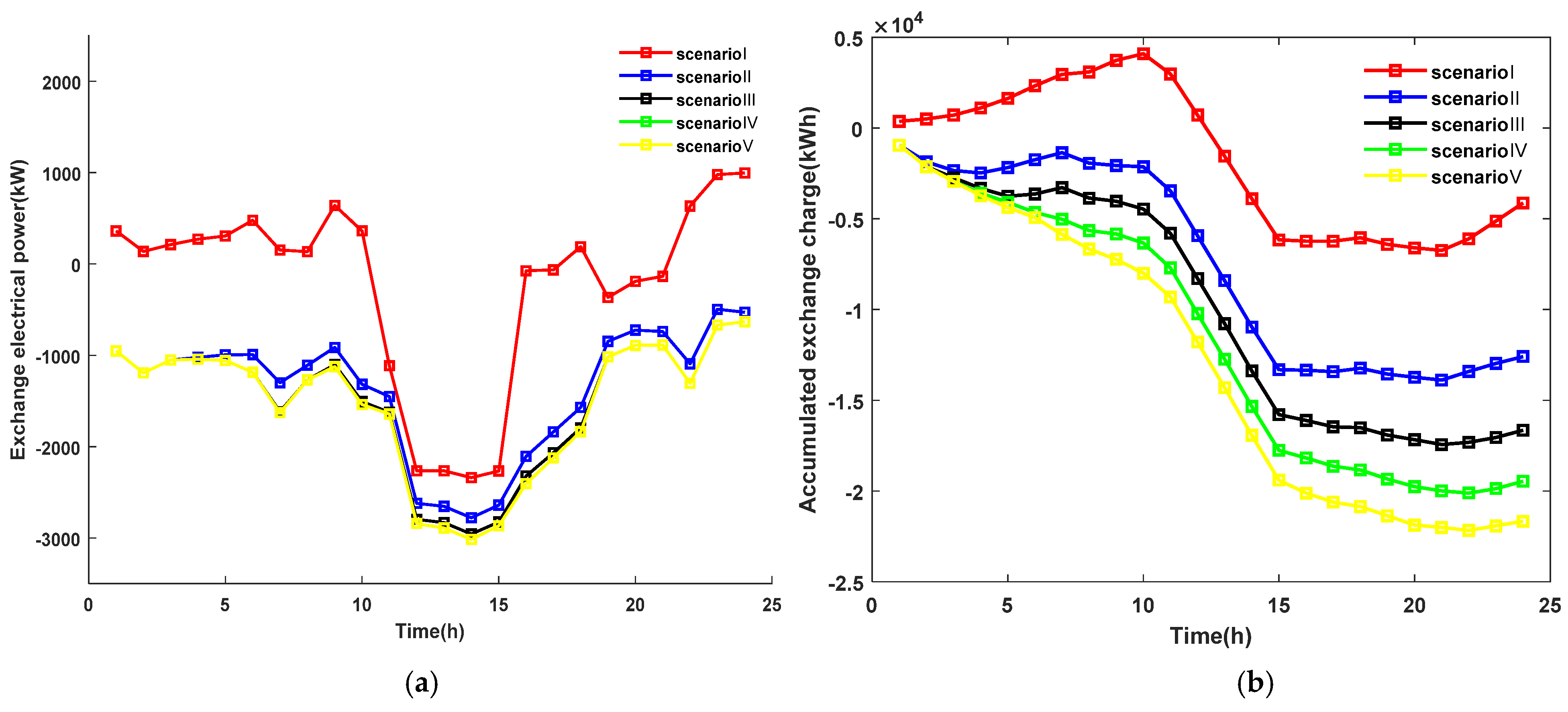
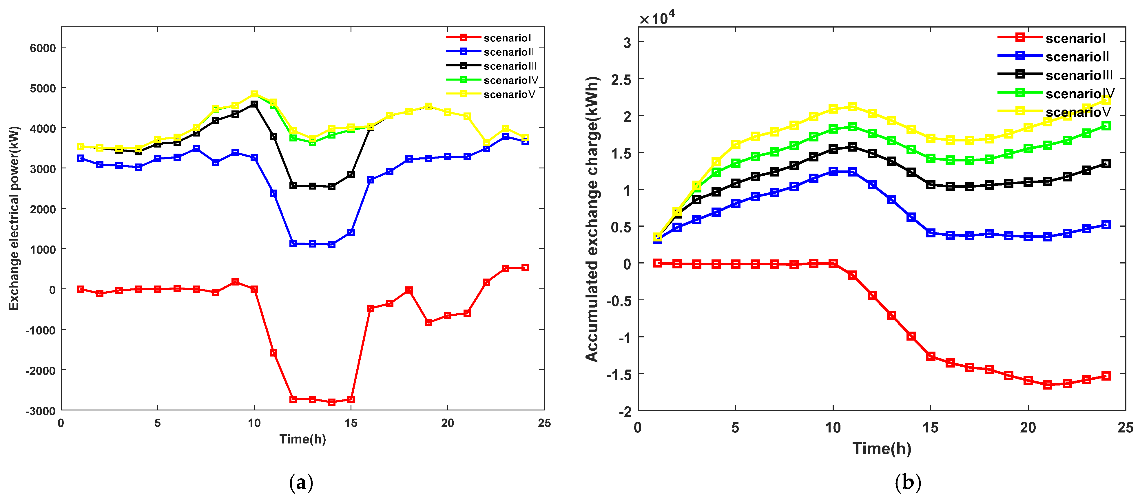
5.2.1. Impacts of Wind and PV Uncertainties on the IES’s Adjustable Capacity Range

In this section, the impact of wind and solar output uncertainty and demand response on the adjustable capacity range of the IES based on chance-constrained planning is comprehensively considered, but since wind and solar abandonment penalties incur economic constraint costs, the economic cost of the perceived budget is not considered here. The adjustable capacity range of the IES is shown in Figure 3.

From the energy supply side, the wind power fluctuated a little at moments 0–9, while the PV power was low. Overall, the wind and PV power outputs were relatively stable, and the demand for electricity by the IES was mainly supplied by the superior grid, so the fluctuation in its upper and lower boundaries was low. At moments 10–15, the overall wind and PV power increased. When evaluating the lower boundaries, the IES dissipated the wind and PV power, which caused large downward fluctuations in the lower boundary, while, when assessing the upper boundary, the IES abandoned all wind and PV power because the budget cost was not taken into account, and the electricity demand was still fully supplied by the superior grid, so there was little fluctuation.

From the demand response point of view, when determining the lower boundary of the adjustable capacity, the dispatch instruction from the load-side grid reduced the total demand for electrical energy of the IES, widening the adjustable range of the lower boundary to some extent. Similarly, when solving the upper boundary, the demand for electrical energy of the IES was increased, which broadened the range of the upper boundary’s adjustable capacity.

The deterministic wind and PV output [20] was analyzed in comparison with the IES adjustable capacity range considering the wind uncertainty. A comparison graph is shown in Figure 4.

When evaluating the upper boundary based on the chance constraint planning, the upward fluctuation in the IES’s consumption of wind power output was mainly taken into account, which reduced the IES’s demand for electricity to a certain extent. Therefore, regardless of the interacting electric power or the cumulative interacting electric power, the upper boundary of the IES’s adjustable capacity decreases compared to the deterministic model. In the same way, the lower boundary of the IES’s adjustable capacity also rises.

5.2.2. Impacts of Confidence Levels on the Adjustable Capacity of the IES

We investigated the effects of different confidence levels on the adjustable capacity range of the IES by setting the confidence levels to 0.9, 0.95, and 0.99, and comparing the adjustable capacity range of the IES.

As can be seen in Figure 5, the higher the confidence level, the more confident the decision-making is in the planning scheme, and the more it can effectively cope with the upward and downward volatility of the wind power consumed by the IES. Therefore, the IES is able to consume more wind power, considering its uncertainty, and the range of the IES’s adjustable capacity is smaller.

5.2.3. Consideration of the Impact of Different Anthropogenic Budgetary Costs on the IES’s Adjustable Capacity Range

Since the models for solving the lower boundary are Equations (24) and (25), and the models for solving the upper boundary are Equations (26) and (27), which are different from each other, when the constraints of the artificial economic budget cost are taken into account, in order to be able to study the impact of the economic cost constraints on the range of the IES adjustable capacity in a more detailed way, the upper and lower boundaries can be separately investigated. The specific process is as follows.

Firstly, the optimal economic scheduling model of the IES is constructed, and based on the chance constraint planning, the constraints are established based on the model for solving the upper and lower boundaries of the adjustable capacity, respectively. The Gurobi solver is used to solve the optimal economics of $C_{\mathrm{s}}$ and $C_{\mathrm{x}}$ when the constraints on the upper and lower boundaries of the adjustable capacity are applied, respectively. Then, based on $C_{\mathrm{s}}$ and $C_{\mathrm{x}}$, the relaxation variables ${\epsilon }_s$ and ${\epsilon }_x$ are introduced to relax the economic constraints, respectively, which are applied to the IES model to assess the adjustable capacity. Finally, based on the different relaxation variables, the ranges of the adjustable capacities under different economic constraints are investigated (

Table 1. Scenarios with different relaxation variables.

Scenario	Upper Boundary Relaxation Variables	Lower Boundary Relaxation Variables
I	0	0
II	0.05	0.015
III	0.1	0.03
IV	0.15	0.045
V	0.2	0.06

).

The economic constraints after the introduction of the slack variables can be expressed separately, as follows:

$$C_{\mathrm{total}}\le (1+{\epsilon }_s)C_{\mathrm{s}}$$

(28)

$$C_{\mathrm{total}}\le (1+{\epsilon }_{\mathrm{x}})C_{\mathrm{x}}$$

(29)

The ranges of the adjustable capacity under different economic budget constraints are shown in Figure 6 and Figure 7, which compare the lower and upper boundaries of the IES’s adjustable capacity under different economic constraints, respectively.

According to the assessment of the lower boundary of the adjustable capacity, the wind and PV power was fully consumed and there was no wind and solar abandonment. The budget cost constraint mainly consisted of the energy purchase cost, demand response compensation cost, energy storage depreciation cost, and carbon emission cost. When the budget cost constraint was low, the IES consumed all wind and PV power and mainly incurred energy purchase costs to meet the demand of the given types of loads. There was not a big difference even when the budget cost constraint was taken into account. In contrast, when determining the upper boundary, due to the high cost of wind and PV abandonment, the IES was more inclined to consume wind and PV power, reducing the power purchase cost from wind and PV abandonment. When the budget cost was insufficient, the IES was more inclined to consume wind power and reduce the power purchase cost and the carbon emission cost generated by the power purchase. Meanwhile, when the budget was sufficient, the IES generated wind and PV abandonment and purchased more electricity and natural gas from the higher-level supply system. Therefore, the economic constraints had a larger impact on the upper boundary of the adjustable capacity, and the difference in the upper boundary was larger under different economic constraints. In summary, the range of the adjustable capacity of the IES was narrower when economic constraints were taken into account.

6. Conclusions

This study proposed a method for assessing the adjustable capacity range of IESs based on chance constraints and taking into account the uncertainty of wind and PV output, which can assess the upper and lower boundaries of an IES’s demand for electricity from a day-ahead perspective. In other words, when the higher-level grid needs to dispatch the IES’s operation mode, it can do so by evaluating the IES’s adjustable capacity range.

The external power demand of the IES was taken as the objective function, and an adjustable capacity assessment model was established with the operation constraints, power balance constraints, and economic constraints of each device in the system. The MATLAB/Yalmip R20230622/Gurobi solver was used to solve the problem. Based on this assessment method, the impacts of the uncertainty of wind and PV output, confidence level, and budget cost constraints on the adjustable capacity range of the IES were investigated by setting up comparisons with different scenarios. The effectiveness of the method was verified, and the following conclusions were drawn:

(1)

The modeling of the IES is similar to that of virtual energy storage, which has multiple factors that can affect its adjustable capacity range, such as the uncertainty of renewable energy output, multiple storage devices, and demand response. By evaluating the adjustable capacity range of the IES, the higher-level grid is able to be more flexible in adjusting its operating status, thus achieving better economic output.

(2)

The chance-constrained planning method was used to consider the volatility of renewable energy output during IES operation and to assess the maximum upward and downward ranges of the IES’s adjustability within the confidence level allowed, so as to provide a reliable reference for decision makers when scheduling them. When the confidence level is higher, the decision maker has more confidence in the IES to consume renewable energy, the amount of power purchased from the higher-level grid will be lower, and the adjustable capacity range will be smaller.

(3)

During operation, the IES incurs various operating costs, such as the cost of energy purchase, the cost of wind and PV power abandonment, the depreciation cost of energy storage devices, the cost of carbon emissions, the cost of demand response compensation, etc., which often cannot be ignored in its actual operation process, limiting the IES’s adjustable capacity. When the budget is more sufficient, the adjustable capacity range is larger, which indicates that the extra regulation capacity provided by the IES to the higher-level grid will incur extra operating costs. The IES can adjust its adjustable capacity by changing the budget to make it more competitive in the market.

This study has made some progress in the assessment of the tunable capability of IESs, but there are still some considerations lacking, and further research can be carried out in the following aspects:

(1)

Regarding the output prediction of wind and photovoltaic power, we could consider incorporating the machine learning method to make more accurate predictions in further work.

(2)

This study was only an evaluation of a single IES. In the future, multi-microgrid systems that consider information exchange systems could be added to evaluate various indicators of multiple integrated energy networks.

References

1. Wang, W.; Yuan, B.; Sun, Q.; Roinald, W. Application of energy storage in integrated energy systems—A solution to fluctuation and uncertainty of renewable energy. J. Energy Storage 2022, 52, 104812. [Google Scholar] [CrossRef]
2. U.S. Department of Energy. U.S. Energy Information Administration. Annual Energy Outlook. 2019. Available online: http://www.eia.gov/outlooks/aeo/pdf/aeo2019.pdf (accessed on 1 October 2023).
3. Wang, C.; Tian, T.; Xu, Z.; Cheng, S.; Liu, S.; Chen, R. Optimal management for grid-connected three/single-phase hybrid multimicrogrids. IEEE Trans. Sustain. Energy 2019, 11, 1870–1882. [Google Scholar] [CrossRef]
4. Xi, L.; Zhang, Z.; Yang, B.; Huang, L.; Yu, T. Wolf pack hunting strategy for automatic generation control of an islanding smart distribution network. Energy Convers. Manag. 2016, 122, 10–24. [Google Scholar] [CrossRef]
5. Wang, C.; Li, X.; Tian, T.; Xu, Z.; Chen, R. Coordinated control of passive transition from grid-connected to islanded operation for three/single-phase hybrid multimicrogrids considering speed and smoothness. IEEE Trans. Ind. Electron. 2019, 67, 1921–1931. [Google Scholar] [CrossRef]
6. Zhu, B.; Ding, F.; Vilathgamuwa, D.M. Coat circuits for DC–DC converters to improve voltage conversion ratio. IEEE Trans. Power Electron. 2020, 35, 3679–3687. [Google Scholar] [CrossRef]
7. Jiang, X.; Li, Q.; Yang, Y.; Zhang, L.; Liu, X.; Ning, N. Optimization of the operation plan taking into account the flexible resource scheduling of the integrated energy system. Energy Rep. 2022, 8, 1752–1762. [Google Scholar] [CrossRef]
8. Liu, J.; Ma, L.; Wang, Q. Energy management method of integrated energy system based on collaborative optimization of distributed flexible resources. Energy 2023, 264, 125981. [Google Scholar] [CrossRef]
9. Zheng, J.; Kou, Y.; Li, M.; Wu, Q. Stochastic optimization of cost-risk for integrated energy system considering wind and solar power correlated. J. Mod. Power Syst. Clean Energy 2019, 7, 1472–1483. [Google Scholar] [CrossRef]
10. Ceseña, E.A.M.; Mancarella, P. Energy systems integration in smart districts: Robust optimisation of multi-energy flows in integrated electricity, heat and gas networks. IEEE Trans. Smart Grid 2018, 10, 1122–1131. [Google Scholar] [CrossRef]
11. Fan, G.; Peng, C.; Wang, X.; Wu, P.; Yang, Y.; Sun, H. Optimal scheduling of integrated energy system considering renewable energy uncertainties based on distributionally robust adaptive MPC. Renew. Energy 2024, 226, 120457. [Google Scholar] [CrossRef]
12. Zhang, Y.; Zheng, F.; Shu, S.; Le, J.; Zhu, S. Distributionally robust optimization scheduling of electricity and natural gas integrated energy system considering confidence bands for probability density functions. Int. J. Electr. Power Energy Syst. 2020, 123, 106321. [Google Scholar] [CrossRef]
13. Tan, Z.; Tan, Q.; Yang, S.; Ju, L.; De, G. A robust scheduling optimization model for an integrated energy system with P2G based on improved CVAR. Energies 2018, 11, 3437. [Google Scholar] [CrossRef]
14. Yun, Y.; Zhang, D.; Yang, S.; Li, P.; Yan, J. Low-carbon optimal dispatch of integrated energy system considering the operation of oxy-fuel combustion coupled with power-to-gas and hydrogen-doped gas equipment. Energy 2023, 283, 129127. [Google Scholar] [CrossRef]
15. Sun, Q.; Wang, X.; Liu, Z.; Mirsaeidi, S.; He, J.; Pei, W. Multi-agent energy management optimiza-tion for integrated energy systems under the energy and carbon co-trading market. Appl. Energy 2022, 324, 119646. [Google Scholar] [CrossRef]
16. Wang, R.; Wen, X.; Wang, X.; Fu, Y.; Zhang, Y. Low carbon optimal operation of integrated energy system based on carbon capture technology, LCA carbon emissions and ladder-type carbon trading. Appl. Energy 2022, 311, 118664. [Google Scholar] [CrossRef]
17. Fan, M.; Cao, S.; Lu, S. Optimal allocation of multiple energy storage in the integrated energy system of a coastal nearly zero energy community considering energy storage priorities. J. Energy Storage 2024, 87, 111323. [Google Scholar] [CrossRef]
18. Li, M.; Qin, J.; Han, Z.; Niu, Q. Low-carbon economic optimization method for integrated energy systems based on life cycle assessment and carbon capture utilization technologies. Energy Sci. Eng. 2023, 11, 4238–4255. [Google Scholar] [CrossRef]
19. Liu, H.; Zhao, Y.; Gu, C.; Ge, S.; Yang, Z. Adjustable capability of the distributed energy system: Definition, framework, and evaluation model. Energy 2021, 222, 119674. [Google Scholar] [CrossRef]
20. Li, Y.; Li, R.; Shi, L.; Wu, F.; Zhou, J.; Liu, J.; Lin, K. Adjustable Capability Evaluation of Integrated Energy Systems Considering Demand Response and Economic Constraints. Energies 2023, 16, 8048. [Google Scholar] [CrossRef]
21. Wang, Y.; Wang, Y.; Huang, Y.; Yu, H.; Du, R.; Zhang, F.; Zhang, F.; Zhu, J. Optimal scheduling of the regional integrated energy system considering economy and environment. IEEE Trans. Sustain. Energy 2018, 10, 1939–1949. [Google Scholar] [CrossRef]
22. Pan, C.; Jin, T.; Li, N.; Wang, G.; Hou, X.; Gu, Y. Multi-objective and two-stage optimization study of integrated energy systems considering P2G and integrated demand responses. Energy 2023, 270, 126846. [Google Scholar] [CrossRef]
23. Wang, C.; Chen, S.; Mei, S.; Ran, C.; Yu, H. Optimal scheduling for integrated energy system considering scheduling elasticity of electric and thermal loads. IEEE Access 2020, 8, 202933–202945. [Google Scholar] [CrossRef]
24. Mohseni, S.; Brent, A.C.; Kelly, S.; Browne, W.N. Demand response-integrated investment and operational planning of renewable and sustainable energy systems considering forecast uncertainties: A systematic review. Renew. Sustain. Energy Rev. 2022, 158, 112095. [Google Scholar] [CrossRef]
Figure 1. IES diagram of multiple input–output ports.
Processes 12 02672 g001
Figure 2. IES structure diagram [20].
Processes 12 02672 g002
Figure 3. Upper and lower boundaries of exchange power and accumulated exchange energy (a,b).
Processes 12 02672 g003
Figure 4. Adjustable capacity comparisons (a,b).
Processes 12 02672 g004
Figure 5. Adjustable capacity at different confidence levels (a,b).
Processes 12 02672 g005
Figure 6. Lower boundaries of exchange power and accumulated exchange energy in different scenarios (a,b).
Processes 12 02672 g006
Figure 7. Upper boundaries of exchange power and accumulated exchange energy in different scenarios (a,b).
Processes 12 02672 g007