Pressure Transient Analysis for Fractured Shale Gas Wells Using Trilinear Flow Model

Abstract

Shale gas, a low-permeability, unconventional resource, requires horizontal drilling and multi-stage fracturing for commercial production. This study develops a trilinear flow model for fractured horizontal wells in shale gas formations, incorporating key mechanisms such as adsorption, desorption, diffusion, wellbore storage, and skin effects. The model delineates seven distinct flow regimes, providing insights into gas migration processes and the factors controlling production. Sensitivity analyses reveal that desorption plays a critical role under low-pressure and low-production conditions, significantly enhancing gas transfer rates from the matrix to the fracture network and contributing to overall production. Monte Carlo simulations further highlight the variability in pressure responses under different input conditions, offering a comprehensive understanding of the model’s behavior in complex reservoir environments. These findings advance the characterization of shale gas flow dynamics and inform the optimization of production strategies.

1. Introduction

Shale gas reservoirs are widely distributed across the globe and possess significant development potential. Preliminary estimates suggest that the total resource volume of global shale gas is nearly equivalent to the combined proven reserves of tight gas and coalbed methane. On average, the permeability of shale reservoirs that have not undergone hydraulic fracturing is typically less than 0.1 mD. This low permeability makes the commercial development of unconventional oil and gas reliant on advanced techniques such as multistage hydraulic fracturing and horizontal drilling. The fracture networks created post-fracturing enhance the heterogeneity of shale reservoirs [1]. Moreover, the presence of organic matter in both dissolved and adsorbed forms further complicates the transport mechanisms within these formations [2]. Given that the drilling, completion, and operational costs of horizontal wells are significantly higher than those of vertical wells, accurately estimating the production capacity of individual wells is essential for optimizing drilling and fracturing designs to achieve economic feasibility. Consequently, research on fluid transport mechanisms considering the pore space and scale of the reservoir, as well as the theory of unstable flow in horizontal wells, is of paramount importance.

Analytical or semi-analytical models are often the preferred approach for evaluating the production capacity of oil and gas wells. First, compared to traditional decline curve methods, which rely solely on production data, analytical and semi-analytical models integrate fluid flow mechanisms with various reservoir properties related to geological characteristics [3]. Second, in contrast to detailed geological modeling and numerical reservoir simulation methods, analytical and semi-analytical approaches do not encounter convergence issues, offering greater computational efficiency, particularly for large-scale problems involving thousands of wells [4]. Third, unlike numerical solutions, analytical and semi-analytical solutions are explicit and provide clearer parameters, making them more practical for sensitivity analysis and flow characterization.

In 1986, Lee et al. [5] first proposed the trilinear flow model to study pressure response in a large reservoir with finite-conductivity vertical fractures. This model was notable for accounting for the influence of fracture spacing and conductivity on the pressure response curve. Later, Brown (2009) and Ozkan (2011) developed a trilinear model to simulate pressure-transient and production behaviors in fractured horizontal wells within unconventional reservoirs. This model integrated the fluid flow across the matrix reservoir, hydraulic fractures, and stimulated reservoir volume (SRV), allowing the consideration of fundamental petrophysical properties and unique fluid characteristics across different reservoir components [6,7]. Over the past decade, researchers have built upon the trilinear flow model, applying higher-resolution studies in more segmented regions of gas reservoirs. Stalgorova and Mattar (2012, 2013) extended the trilinear model to a five-region flow model to capture more complex reservoir scenarios. Their model considered flow in both fractured and unfractured areas within the SRV, including flows parallel and perpendicular to fractures, and demonstrated that unfractured SRV (USRV) significantly influences long-term production in typical shale gas wells [8,9]. Subsequently, Zhang (2015), Deng (2015), Zhang (2016), and Haeri (2017) expanded the five-linear model by incorporating nonlinear flow mechanisms in both heterogeneous and homogeneous multi-fracture systems [10,11,12,13]. Zeng (2016, 2017) further developed this into a seven-linear flow model, addressing reservoir heterogeneity along the horizontal wellbore. Results indicated that pressure and production response disparities primarily arise in the later stages, with larger pressure drawdowns and faster production declines occurring under higher-threshold pressure gradients, though this impact is minimal when gradients are low. Other influential parameters, including formation permeability, heterogeneity, fracture length, conductivity, and wellbore storage, were also systematically investigated [14,15]. Zhao and Du (2019, 2020) introduced a mathematical model for a horizontal well in a dual-porosity composite tight gas reservoir with considering the stress–sensitivity effect and unsteady flow between matrix and fractures systems [16,17].

More recently, Wang (2022) described non-Darcy flow behavior in nano/microscale pores using a linear superposition approach and Darcy flow in larger pores and natural or induced fractures in the shale matrix [18]. However, most modeling studies have focused on individual wells, often overlooking the enhanced stimulated reservoir volume (ESRV) and inter-well interference. Addressing this, Guo (2023) derived a new semi-analytical solution for shale gas reservoirs that integrates fracture network heterogeneity and multiple gas transport mechanisms. This model captures gas desorption, diffusion, and viscous flow within the matrix, alongside viscous flow in the fracture system and the properties of the ESRV and SRV. The resulting bottom-hole pressure (BHP) and production dynamics revealed significant differences between multi-well platforms with an ESRV and SRV and the traditional single-well models found in shale reservoirs with homogeneous fracture networks [19]. Qin et al. (2023) developed an integrated approach combining pressure and rate transient analysis for well interference diagnosis considering complex fracture networks [20]. Liang et al. (2024) proposed a semi-analytical model of a directional well based on the assumption of non-uniform flux distribution [21].

Existing models, including linear flow, composite linear flow, trilinear flow, and five-linear flow frameworks, have been widely employed to describe fluid transport in fractured horizontal wells. Linear flow models offer simplicity and analytical tractability, effectively capturing essential flow dynamics. Composite linear models introduce additional flow zones, addressing reservoir heterogeneities with greater precision. Trilinear flow models refine this concept by delineating distinct flow regions for the matrix, fractures, and stimulated zones, while five-linear models further enhance characterization by incorporating additional pathways to represent multi-scale flow behaviors. Despite these advancements, these models primarily rely on geometric flow assumptions and often neglect critical shale gas-specific mechanisms, such as adsorption–desorption and Knudsen diffusion [22]. These mechanisms become particularly significant under low-pressure and low-production conditions, where gas migration from the matrix to the fractures is heavily influenced by desorption processes. As a result, the applicability of these models to shale gas reservoirs is limited, especially when attempting to represent the complex interactions between matrix storage, fracture networks, and unconventional flow regimes.

To overcome these limitations, this study introduces a dual-porosity trilinear flow model that integrates adsorption–desorption and diffusion effects into the analysis of shale gas flow behavior. The proposed model incorporates quasi-steady-state diffusion within the matrix, fracture seepage, wellbore storage, and skin effects, thereby offering a more comprehensive representation of flow dynamics. Using Laplace domain solutions, the model generates dimensionless pressure and pressure derivative curves, enabling the identification of seven distinct flow regimes. Sensitivity analyses highlight the critical influence of parameters such as the desorption coefficient and elastic storage ratio on gas transfer rates and pressure dynamics. By addressing the limitations of existing models, this work provides a robust analytical framework for understanding flow mechanisms and improving production predictions in fractured shale gas reservoirs.

2. Materials and Methods

2.1. Flow Mechanism

Currently, there is significant debate regarding the mechanisms governing gas migration in the shale matrix, and it remains unclear whether gas migration is primarily driven by pressure gradients causing seepage, concentration gradients leading to diffusion, or a combination of both. This study assumes that the migration mechanism in the shale matrix involves both desorption and diffusion, with the quasi-steady-state diffusion process described by Fick’s first law. In the dual-porosity model, Darcy flow and diffusion mechanisms are considered in natural fractures, while hydraulic fractures, due to their high permeability and wide flow channels, are modeled to only account for Darcy flow.

2.1.1. Desorption Mechanism

In shale gas reservoirs, desorption occurs from the surface of kerogen within the shale matrix to microscopic pores. Thus, to accurately describe the desorption process in the shale matrix, parameters beyond standards such as volume and the Langmuir adsorption isotherm are required, including the distribution of kerogen and pressure profiles. Research in this area remains incomplete; therefore, this study considers desorption primarily in the gas flow model for the shale matrix. The desorption of adsorbed gas from the surface of organic pores is a key mechanism for shale gas production. The amount of adsorbed gas depends on the prevailing pressure and adsorption conditions, which can be estimated using the Langmuir isotherm equation, expressed as follows:

$$V={\displaystyle \frac{V_{L}p}{p_L+p}}$$

(1)

where $V$ denotes the amount of gas adsorbed per unit mass of the adsorbent at a given pressure, cm³/g; $V_L$ denotes the maximum adsorption capacity, indicating the maximum quantity of gas that can be adsorbed onto the surface at very high pressures, cm³/g; and $P_L$ is the Langmuir pressure constant, defined as the pressure at which half of the maximum adsorption capacity ($V_L$) is achieved, Pa.

2.1.2. Diffusion Mechanism

When the gas pressure is very low or capillary pore diameter is very small, the mean free path of gas molecules significantly exceeds the pore diameter. Consequently, molecular collisions with pore walls occur more frequently than intermolecular collisions. Under these conditions, the primary resistance to gas diffusion along the pores arises from molecule–wall interactions, a phenomenon known as Knudsen diffusion. Knudsen diffusion in nanopores can be expressed in terms of a pressure gradient and, using the real gas equation of a state, can be reformulated in terms of density. Ignoring viscous effects, the mass flow rate of gas due to diffusion can be described as follows:

$$J_D=D_K\nabla {\rho }_g$$

(2)

where J_D represents the amount of substance that flows through a unit area per unit time, kg/m²·s; $D_K$ denotes the diffusion coefficient, a proportionality constant that describes the ease with which the substance diffuses through the medium, m²/s; and ${\rho }_g$ denotes the density of the gas.

2.1.3. Darcy Flow

The flow in hydraulic fractures within shale gas reservoirs is similar to that in conventional natural gas reservoirs, but additional flow mechanisms may also exist, such as slip effects, high-velocity non-Darcy flow, and stress–sensitivity effects. For this study, these factors are neglected, and it is assumed that only Darcy flow exists in natural fractures. Specifically,

$$v^p={\displaystyle \frac{3.6k}{\mu }}\nabla p$$

(3)

where $v^p$ denotes the gas flow velocity, m/h; $\mu$ denotes the gas viscosity, mPa/s; and $k$ denotes the permeability, D.

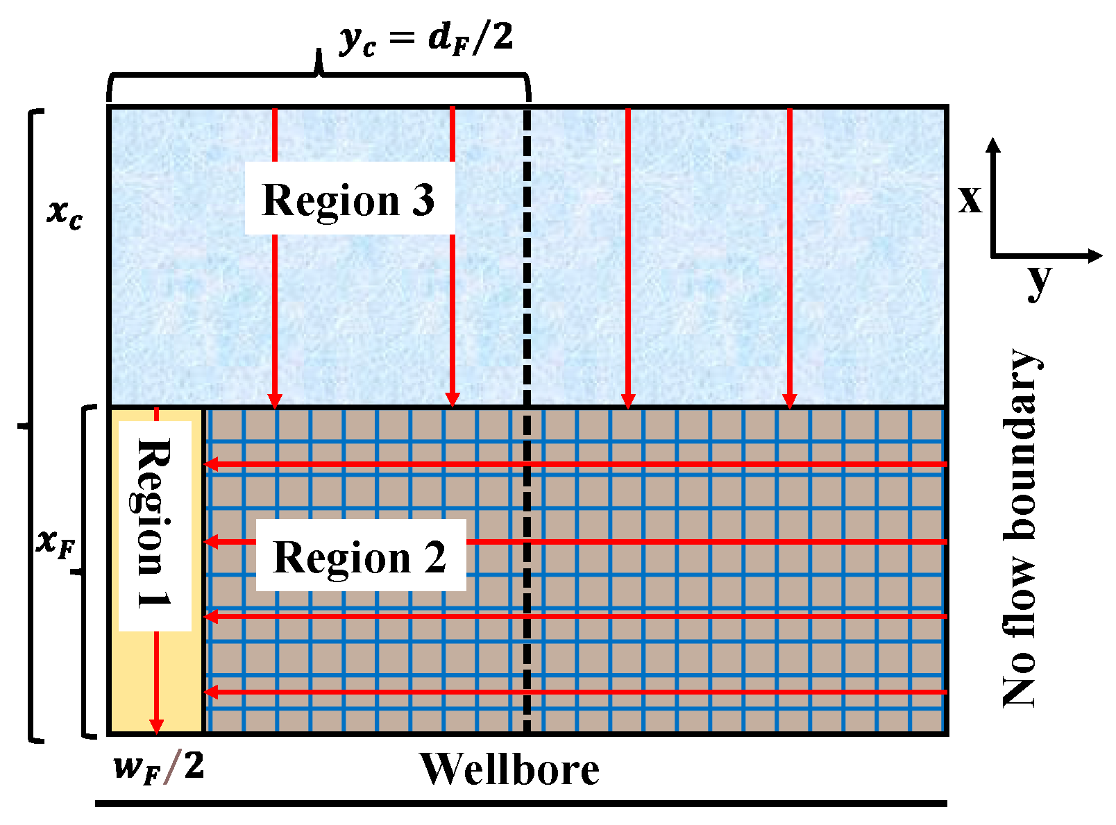
2.2. Physical Model of TriLinear Flow Model for Dual Media

Due to the geometric symmetry of the model, the trilinear flow model considers one-quarter of the reservoir around a single hydraulic fracture, as shown in Figure 1. The flowchart of this study is shown in Figure 2. The reservoir can be divided into three regions based on permeability: the outer region, the inner region, and the fracture region. The outer region is unfractured, while the inner region lies between two hydraulic fractures, containing induced fractures. Fluid flow in each region is linear: linear flow 1 represents flow from the outer to the inner region, linear flow 2 represents flow from the inner region to the fracture region, and linear flow 3 represents flow from the fracture region to the horizontal wellbore. No fluid flows at the midline between the two hydraulic fractures. Let $2y_e$ represent the spacing between fractures, $2x_e$ represent the reservoir length in the x-direction, $2x_F$ represent the fracture length, and $2w_F$ represent the fracture width, with the subscripts O, I, and F corresponding to the outer, inner, and fracture regions, respectively.

The model assumptions are as follows: (1) single-phase isothermal flow, neglecting capillary forces and gravity; (2) a closed outer boundary of the gas reservoir, with hydraulic fractures modeled as symmetric vertical planar fractures relative to the horizontal well, equal spacing between fractures, and uniform physical properties; (3) constant pressure within the horizontal wellbore; (4) no additional pressure drop across the inner and outer cross-sections, with an inner region height equal to the fracture half-length $x_F$, a fracture width $w_F$, a reservoir thickness $h$, fracture spacing $d_F$, and no fluid flow at $d_F/2$ between the two fractures; (5) both the inner and outer regions consist of naturally fractured reservoirs, adopting a dual-porosity model; (6) similarly to traditional pressure transient analysis models, this study simplifies assumptions and reduces computational complexity by not considering the anisotropy of permeability.

Natural fractures in dual-porosity models are typically described with three matrix shapes: slab, spherical, and cubic, simulating one-dimensional, two-dimensional, and three-dimensional flows, respectively. Moghadam et al. demonstrated that the matrix shape does not affect the overall flow pattern in dual-porosity models [23]. In this study, cylindrical matrix blocks are used to characterize quasi-steady-state flow within the matrix system.

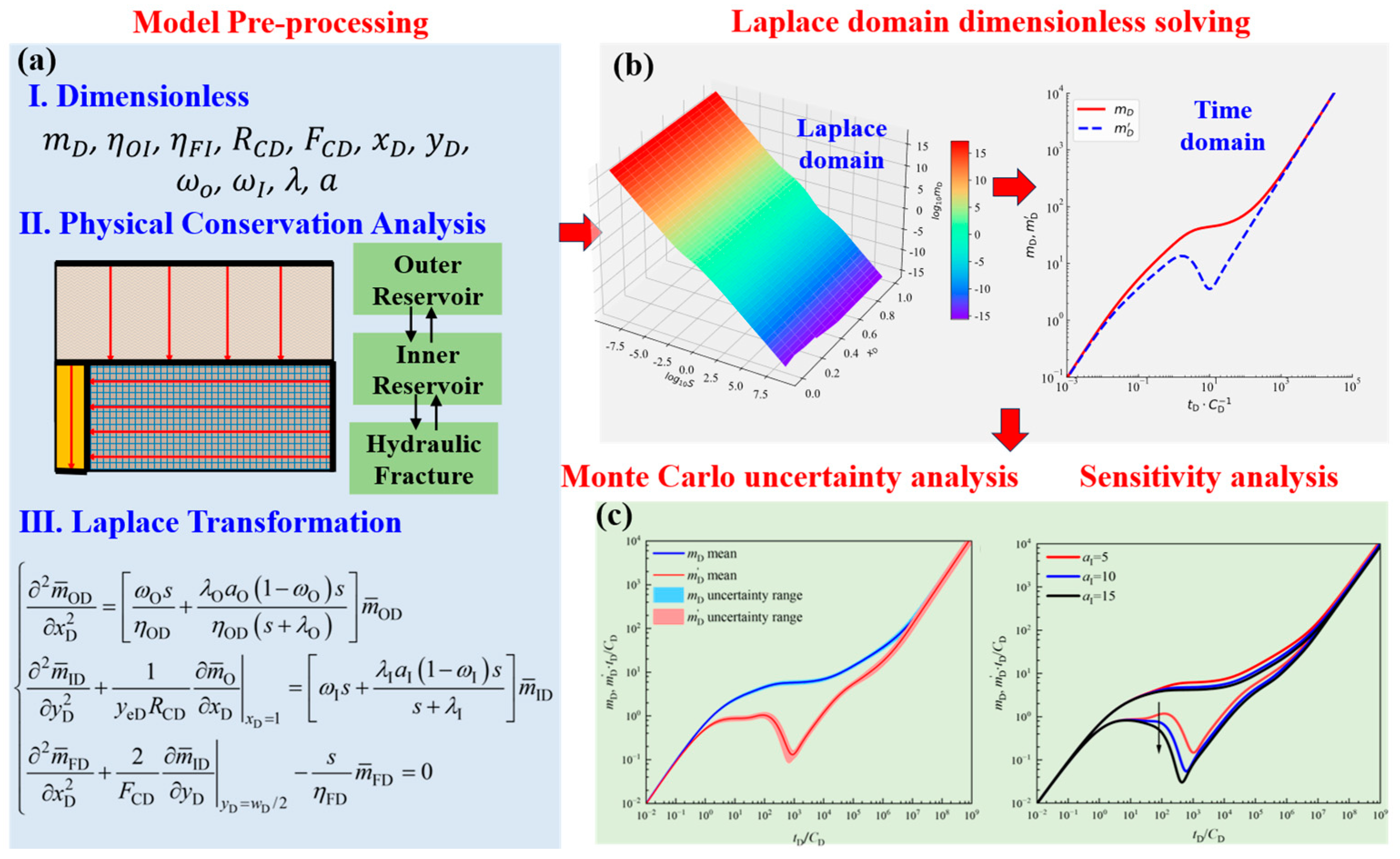
2.3. Mathematical Model

To simplify the mathematical model and enable a unified expression of physical processes across different scales, dimensionless variables and associated coefficients are defined as shown in the following

Table 1. Definitions of dimensionless variables and related parameters.

Variables	Definition
Dimensionless pseudo-pressure	$m_D={\displaystyle \frac{k_I{h}_I}{1.2734\times {10}^{-2}{q}_{F}T}}\left[m\left(p_i\right)-m(p)\right]$
Time	$t_D={\displaystyle \frac{{\eta }_I}{x_F^2}}t$
Pseudo-pressure	$m(p)=2{\displaystyle {\int }_{p_b}^p\frac{p}{\mu z}}dp$
x-direction coordinate	$x_D={\displaystyle \frac{x}{x_F}}$
y-direction coordinate	$y_D={\displaystyle \frac{y}{x_F}}$
Diffusivity ratio	${\eta }_{OD}={\displaystyle \frac{{\eta }_O}{{\eta }_I}}$$,{\eta }_{FD}={\displaystyle \frac{{\eta }_F}{{\eta }_I}}$
Hydraulic fracture conductivities	$F_{CD}={\displaystyle \frac{k_F{w}_F}{k_I{x}_F}}$
Reservoir conductivities	$R_{CD}={\displaystyle \frac{k_I{x}_F}{k_O{y}_e}}$
Storativity	${\omega }_o={\displaystyle \frac{\mu {(\phi c)}_O}{{\sigma }_O}}$$,{\omega }_I={\displaystyle \frac{\mu {(\phi c)}_I}{{\sigma }_I}}$
Inter-porosity coefficients	$\lambda ={\displaystyle \frac{x_F^2}{{\eta }_I\tau }}$
Adsorption index	$a={\displaystyle \frac{1.2734\times {10}^{-2}{q}_{F}T}{k_I{h}_I}}{\displaystyle \frac{q_L{m}_L}{\left(m_i+m_L\right)\left(m+m_L\right)}}$
Associated coefficients	${\sigma }_O=\mu {(\phi c)}_O+{\displaystyle \frac{k_I{h}_t{p}_{sc}}{0.6367\times {10}^{-2}{T}_{sc}{q}_F}}$
Concentration of gas	$V_{OD}=V_i-V_O$

where $k_I$ denotes the permeability of the inner region, mD; $h_I$ denotes the thicknesses of the inner region, m; $q_F$ denotes the quarter production rate from a single fracture, m³/d; $\eta$ denotes the diffusivity, m²/h; $x_F$ denotes the hydraulic fracture half-length, m; $p_b$ denotes the bubble point pressure, bar; and z denotes the real gas compressibility factor, dimensionless.

:

2.3.1. Outer Region

1.

Quasi-steady-state diffusion flow equation in matrix system

The model developed in this study disregards Darcy flow within the matrix region driven by pressure gradients, instead focusing on diffusion mechanisms induced by concentration gradients. Only the temporal variation in concentration is considered, with the rate of change in the shale gas concentration within the matrix proportional to the concentration difference between the matrix and the fracture. Accordingly, the motion equation can be expressed by Fick’s first law:

$${\displaystyle \frac{\partial V_O}{\partial t}}={\displaystyle \frac{1}{{\tau }_O}}\left(V_{OE}-V_O\right)$$

(4)

where ${\tau }_O$ denotes the time required for the shale gas concentration to reach equilibrium, h; $V_O$ denotes the under-the-standard condition, and the amount of shale skeleton diffusion per unit volume in the outer zone is m³/m³; $V_{OE}$ denotes the volume concentration of shale gas at the interface between the matrix system and the fracture system, which is in equilibrium with the pressure in the fracture, m³/m³.

According to the parameters defined in Table 1, the dimensions from Equation (4) can be expressed as follows:

$${\displaystyle \frac{\partial V_{OD}}{\partial t_D}}={\lambda }_O\left(V_{OED}-V_{OD}\right)$$

(5)

$$V_{OED}=V_i-V_{OE}={\displaystyle \frac{q_L{m}_i}{m_i+m_L}}-{\displaystyle \frac{q_L{m}_O}{m_O+m_L}}=a_O{m}_{OD}$$

(6)

where $a_O$ denotes the adsorption index in the outer region.

Equations (5) and (6) are written by the Laplace transform:

$${\overline{V}}_{OD}={\displaystyle \frac{{\lambda }_O{a}_O}{s+{\lambda }_O}}{\overline{m}}_{OD}$$

(7)

2.

Darcy’s seepage equation in fracture systems

By combining Fick’s first law of diffusion with the Darcy law of flow, a continuity equation is established for the fracture system:

$${\displaystyle \frac{\partial }{\partial x}}\left({\rho }_{gO}{\displaystyle \frac{3.6k_O}{\mu }}{\displaystyle \frac{\partial p_O}{\partial x}}\right)={\displaystyle \frac{\partial }{\partial t}}\left({\varphi }_O{\rho }_{gO}+{\rho }_{gsc}{V}_O\right)$$

(8)

where ${\rho }_{gO}$ denotes the gas density of the outer region, kg/m³; $k$ denotes the permeability, D; $\mu$ denotes the gas viscosity, mPa·s; $p$ denotes the gas pressure, MPa; $\varphi$ denotes the porosity, %; and ${\rho }_{gsc}$ denotes the gas density in standard conditions, kg/m³.

The gas density can be expressed by the equation of state as follows:

$${\rho }_{gm}={\displaystyle \frac{p_{m}M}{ZRT}}$$

(9)

where $M$ denotes the gas molar mass, kg/kmol; $R$ is the molar constant, J/(Kmol-K); and $T$ is the gas reservoir temperature, K.

By coupling the quasi-steady-state diffusion equation for the matrix system with the Darcy flow equation for the fracture system, a dimensionless composite continuity equation for the outer region is derived as follows:

$${\displaystyle \frac{{\partial }^2{\overline{m}}_{OD}}{\partial x_D^2}}=\left[{\displaystyle \frac{{\omega }_{O}s}{{\eta }_{OD}}}+{\displaystyle \frac{{\lambda }_O{\alpha }_O(1-{\omega }_O)s}{{\eta }_{OD}(s+{\lambda }_O)}}\right]{\overline{m}}_{OD}$$

(10)

The mathematical modeling of Laplace-transformed dimensionless integrated seepage considering internal and external boundary conditions can be expressed as follows:

$$\{\begin{array}{l}{\displaystyle \frac{{\partial }^2{\overline{m}}_{OD}}{\partial x_D^2}}=\left[{\displaystyle \frac{{\omega }_{O}s}{{\eta }_{OD}}}+{\displaystyle \frac{{\lambda }_O{a}_O\left(1-{\omega }_O\right)s}{{\eta }_{OD}\left(s+{\lambda }_O\right)}}\right]{\overline{m}}_{OD}\hfill \\ {{\displaystyle \frac{\partial {\overline{m}}_{OD}}{\partial x_D}}|}_{x_D=x_{eD}}=0\hfill \\ {{\overline{m}}_{OD}|}_{x_D=1}={{\overline{m}}_{ID}|}_{x_D=1}\hfill \end{array}$$

(11)

The solution of the seepage model in the Laplace space domain is obtained as follows:

$${\overline{m}}_{OD}={{\overline{m}}_{DD}|}_{x_D=1}{\displaystyle \frac{\cosh \left[\sqrt{f_O(s)}\left(x_{eD}-x_D\right)\right]}{\cosh \left[\sqrt{f_O(s)}\left(x_{eD}-1\right)\right]}}$$

(12)

where $f_O(s)={\displaystyle \frac{{\omega }_{O}s}{{\eta }_{OD}}}+{\displaystyle \frac{{\lambda }_O{\alpha }_O(1-{\omega }_O)s}{{\eta }_{OD}(s+{\lambda }_O)}}$.

2.3.2. Inter-Region

Similarly to the matrix system in the outer region, a quasi-steady-state diffusion flow equation for the matrix system is established based on Fick’s first law of diffusion. By integrating Fick’s diffusion law, Darcy’s law, and the flow rate from the outer region into the inner region model, a flow equation for the fracture system in the inner region is developed. By jointly solving the quasi-steady-state diffusion equation for the matrix system and the Darcy flow equation for the fracture system, the dimensionless composite continuity equation for the inner region is derived as follows:

$${\displaystyle \frac{{\partial }^2{\overline{m}}_{ID}}{\partial y_D^2}}+{{\displaystyle \frac{1}{y_{eD}{R}_{CD}}}{\displaystyle \frac{\partial {\overline{m}}_O}{\partial x_D}}|}_{x_{D=1}}=\left[{\omega }_{I}s+{\displaystyle \frac{{\lambda }_1{a}_I\left(1-{\omega }_I\right)s}{s+{\lambda }_I}}\right]{\overline{m}}_{ID}$$

(13)

Considering the internal and external boundary conditions, the Laplace-transformed unfactored integrated seepage mathematical model can be expressed as follows:

$$\{\begin{array}{l}{\displaystyle \frac{{\partial }^2{\overline{m}}_{ID}}{\partial y_D^2}}+{{\displaystyle \frac{1}{y_{eD}{R}_{CD}}}{\displaystyle \frac{\partial {\overline{m}}_O}{\partial x_D}}|}_{x_D=1}=\left[{\omega }_{I}s+{\displaystyle \frac{{\lambda }_I{a}_I\left(1-{\omega }_I\right)s}{s+{\lambda }_I}}\right]{\overline{m}}_{ID}\hfill \\ {{\displaystyle \frac{\partial {\overline{m}}_{ID}}{\partial y_D}}|}_{y_D=y_D}=0\hfill \\ {{\overline{m}}_{ID}|}_{y_D={\omega }_D/2}={{\overline{m}}_{FD}|}_{y_D=w_D/2}\hfill \end{array}$$

(14)

The solution of the integrated seepage mathematical model of the outer zone is obtained by associating the solution of the inner zone seepage mathematical model in the Laplace-space domain as follows:

$${\overline{m}}_{ID}={{\overline{m}}_{FD}|}_{y_D=w_D/2}{\displaystyle \frac{\cosh \left[\sqrt{{\alpha }_I}\left(y_{eD}-y_D\right)\right]}{\cosh \left[\sqrt{{\alpha }_I}\left(y_{eD}-w_D/2\right)\right]}}$$

(15)

where $f_1(s)={\omega }_{I}s+{\displaystyle \frac{{\lambda }_I{a}_I\left(1-{\omega }_I\right)s}{s+{\lambda }_I}}$, ${\beta }_I=\sqrt{f_O(s)}\tanh \left[\sqrt{f_O(s)}\left(x_{eD}-1\right)\right]$, and ${\alpha }_I={\displaystyle \frac{{\beta }_I}{R_{CD}{y}_{eD}}}+f_I(s)$.

2.3.3. Hydraulic Fracture

The desorption and diffusion mechanisms of shale gas are not considered in the hydraulic fracture, which is a one-dimensional Darcy seepage in the x-direction and is obtained by considering the equation of state and the proposed pressure, and is obtained by the dimensionless and Laplace transforms:

$${\displaystyle \frac{{\partial }^2{\overline{m}}_{FD}}{\partial x_D}}+{{\displaystyle \frac{2}{F_{CD}}}{\displaystyle \frac{\partial {\overline{m}}_{ID}}{\partial y_D}}|}_{y_D=w_D/2}={\displaystyle \frac{s}{{\eta }_{FD}}}{\overline{m}}_{FD}$$

(16)

Considering the internal and external boundary conditions, the Laplace-transformed unfactored integrated seepage mathematical model can be expressed as follows:

$$\{\begin{array}{l}{\displaystyle \frac{{\partial }^2{\overline{m}}_{FD}}{\partial x_D^2}}+{{\displaystyle \frac{2}{F_{CD}}}{\displaystyle \frac{\partial {\overline{m}}_{ID}}{\partial y_D}}|}_{y_D=w_D/2}-{\displaystyle \frac{s}{{\eta }_{FD}}}{\overline{m}}_{FD}=0\hfill \\ {{\displaystyle \frac{\partial {\overline{m}}_{FD}}{\partial x_D}}|}_{x_D=1}=0\hfill \\ {{\displaystyle \frac{\partial {\overline{m}}_{FD}}{\partial x_D}}|}_{x_D=0}=-{\displaystyle \frac{\pi }{F_{CD}s}}\hfill \end{array}$$

(17)

The solution of the mathematical model of seepage in the inner zone is obtained by associating the mathematical model of hydraulic fracture in the Laplace-space domain and is solved as follows:

$${\overline{m}}_{FD}={\displaystyle \frac{\pi }{F_{CD}s\sqrt{{\alpha }_F}}}{\displaystyle \frac{\cosh \left[\sqrt{{\alpha }_F}\left(1-x_D\right)\right]}{\sinh \left(\sqrt{{\alpha }_F}\right)}}$$

(18)

where ${\beta }_F=\sqrt{{\alpha }_I}\tanh \left[\sqrt{{\alpha }_I}\left(y_{eD}-w_D/2\right)\right]$ and ${\alpha }_F={\displaystyle \frac{2{\beta }_F}{F_{CD}}}+{\displaystyle \frac{s}{{\eta }_{FD}}}$.

Without considering the wellbore storage and skin effect conditions, the pressure in the hydraulic fracture at x = 0 is the bottomhole pressure:

$${\overline{m}}_{wD}={\displaystyle \frac{\pi }{F_{CD}s\sqrt{{\alpha }_F}\tanh \left(\sqrt{{\alpha }_F}\right)}}$$

(19)

The wellbore storage and skin effect can be considered a combination of the superposition principle and Duhamel principle, which is expressed in the Laplace-space domain:

$${\overline{m}}_{wD}\left(S_c,C_D\right)={\displaystyle \frac{s{\overline{m}}_{wD}+S_c}{s\left[1+C_{D}s\left(s{\overline{m}}_{wD}+S_c\right)\right]}}$$

(20)

3. Results and Discussion

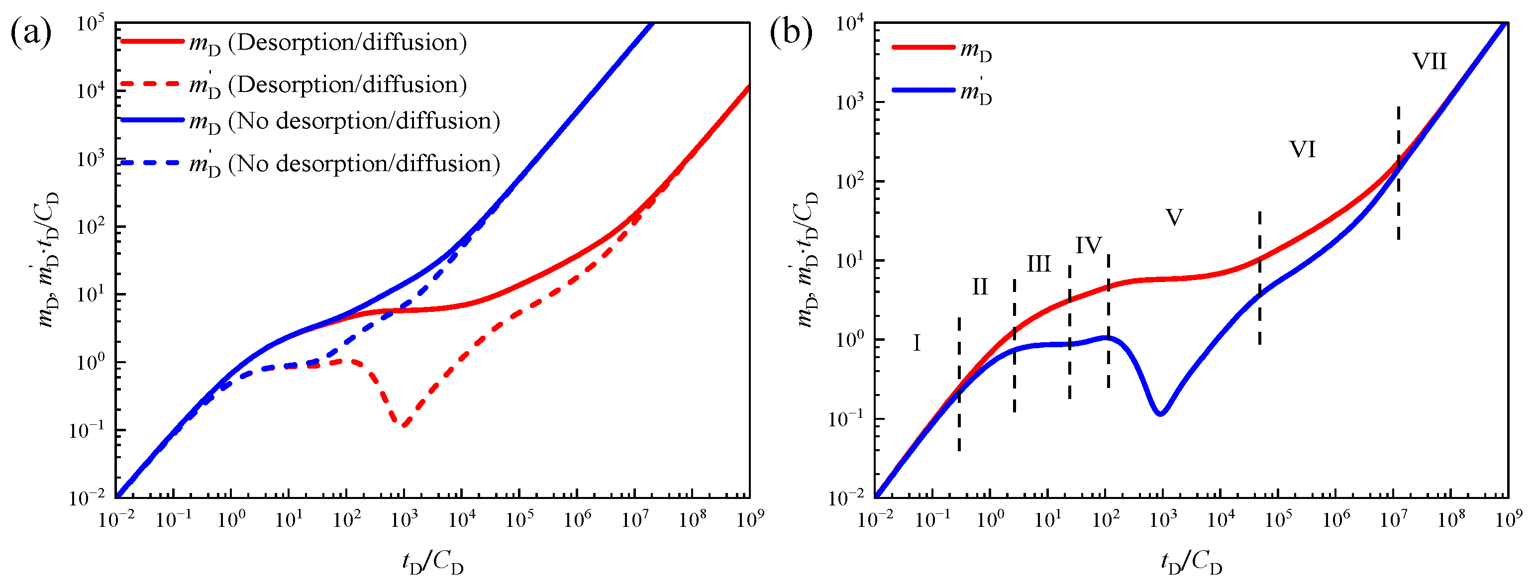
3.1. Flow Regime Division

Parameter combinations were considered, as shown in

Table 2. The parameters of the physical model to be solved.

Parameters	Value	Parameters	Value
$a_I$	6	${\eta }_{FI}$	500
$a_O$	50	${\mathrm{\lambda }}_I$	0.5
${\omega }_o$	0.03	$x_{eD}$	5
${\omega }_I$	0.05	$y_{eD}$	0.5
${\omega }_D$	10−6	$F_{CD}$	0.11
${\lambda }_O$	0.03	$R_{CD}$	15
${\eta }_{OI}$	1.2	$C_D$	10−4
$s_c$	10−2

, and the pressure response curve was drawn using the above analytical solution and Laplace inverse transformation.

To validate the proposed model, we compared the pressure response curves derived from the dual-porosity trilinear flow model, which incorporates adsorption–desorption and diffusion effects, with those generated by the conventional trilinear flow model that neglects these mechanisms, as shown in Figure 3a. The comparison revealed significant differences, particularly under low-pressure and low-production conditions. In the conventional trilinear flow model, the pressure derivative curve exhibits a relatively shallow concave shape, reflecting a simplified fluid exchange process between the matrix and fractures. This simplification arises from the absence of adsorption and desorption effects, which are crucial for regulating the gas transfer rate from the matrix to the fracture system. In contrast, the proposed model demonstrates a more pronounced concavity in the dimensionless pressure derivative curve, highlighting the substantial contribution of desorption to overall flow dynamics. Specifically, the desorption mechanism enhances gas release from the matrix, effectively increasing gas supply to the fracture network and resulting in a delayed pressure decline. These findings underscore the necessity of incorporating adsorption–desorption and diffusion mechanisms to accurately predict the pressure behavior of fractured shale gas reservoirs.

According to the pressure response characteristic curve of the trilinear flow model, the entire shale gas flow process can be divided into seven distinct flow stages, as shown in Figure 3b. These stages provide a detailed depiction of the wellbore effects, fracture–reservoir interactions, and the complex flow behavior of gas within the matrix system:

• Wellbore Storage Stage. In this phase, the dimensionless pressure and dimensionless pressure derivative curves overlap, forming a straight line with a slope of 1. This phase typically has a short duration, primarily governed by the wellbore storage coefficient and skin effect.
• Transition Stage Post-Wellbore Storage. The duration of this stage is still mainly influenced by the wellbore storage coefficient and skin effect, representing the transition of flow from the wellbore to the fractures. The pressure derivative curve deviates, indicating a gradual shift in fluid flow from the wellbore toward interaction with the fractures and the reservoir.
• Bilinear Flow Between Fractures and Reservoir. The pressure derivative curve exhibits a straight line with a slope of 1/4, characteristic of bilinear flow. This reflects the process of fluid flow from the reservoir through the fracture system toward the wellbore. During this stage, the interaction between the fractures and the reservoir is most pronounced.
• Reservoir Linear Flow Stage. The pressure derivative follows a straight line with a slope of 1/2. The duration of this linear flow stage is affected by the permeability of the reservoir and the complexity of the fracture network.
• Desorption and Diffusion Processes in Inner Region Matrix System. This stage is characterized by a concave shape in the dimensionless pressure derivative curve, representing the desorption of gas entering the fracture system through quasi-steady diffusion from the matrix.
• Desorption and Diffusion Processes in Outer Region Matrix System. Similarly to the inner region, this stage reflects the desorption and quasi-steady diffusion of adsorbed and free gas from the matrix to the fractures in the outer region. This stage is typically prolonged due to the slower desorption and diffusion processes in the outer region matrix, significantly impacting the final production.
• System-Wide Quasi-Steady Flow Stage. In this final stage, the dimensionless pressure and pressure derivative curves coalesce and slope upward, forming a straight line with a slope of 1. This indicates that the system flow has reached equilibrium, the fluid flow rate has stabilized, and the pressure differential between the reservoir and fracture systems has gradually balanced.

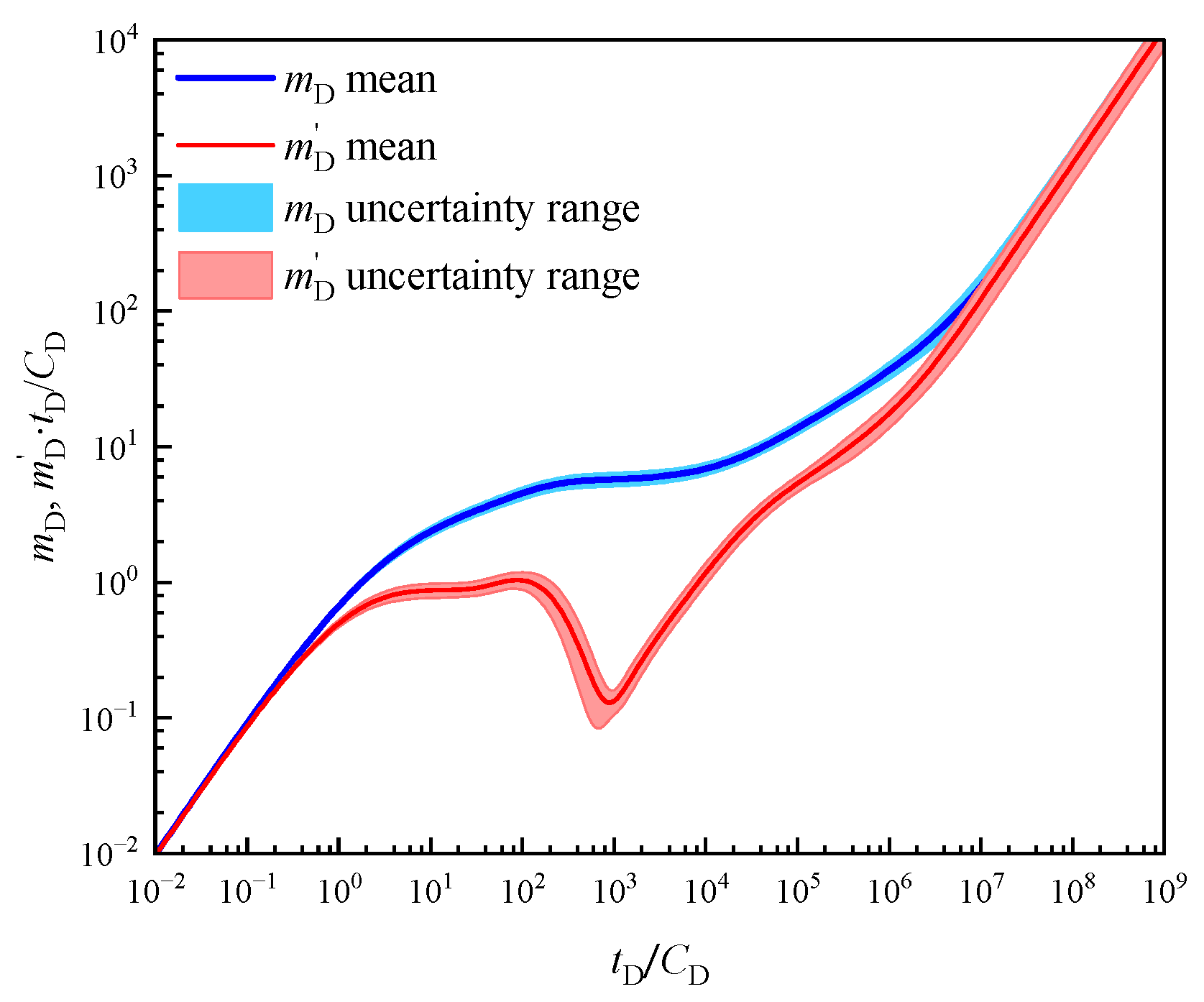
3.2. Monte Carlo Simulation and Uncertainty Analysis

In the shale gas trilinear flow model, the prediction uncertainty is exacerbated by the spatial and temporal variability of several key parameters, as well as the complex relationships between these parameters and the physical properties of the subsurface reservoir. To quantitatively assess the impact of these uncertainties on pressure response curves, this study employs the Monte Carlo simulation (MCS) method.

Monte Carlo simulation is a widely used numerical technique based on random sampling, applied extensively for uncertainty quantification, sensitivity analysis, and risk assessment. The primary advantage of MCS lies in its ability to accurately estimate the probability distribution of system outputs by simulating a large number of different input combinations. In practical applications, the input parameters of many physical models are inherently uncertain, stemming from experimental errors, measurement inaccuracies, or the natural variability of the parameters themselves. By incorporating these uncertainties explicitly through Monte Carlo simulation, we can obtain more reliable output distributions.

3.2.1. Monte Carlo Simulation

In this study, we applied Monte Carlo simulation to the input parameters of the shale gas trilinear flow model. The key model parameters were assumed to follow known probability distributions, derived from prior knowledge or experimental data. For each simulation step, a set of parameters was randomly drawn from these distributions and substituted into the forward model to solve for the corresponding pressure response curve. The specific steps were as follows:

• Parameter Distribution Setup: The probability distributions of the input parameters were first determined, along with their statistical properties (e.g., mean and standard deviation). For each input parameter, we assumed a distribution, such as normal, log-normal, or uniform, depending on the physical context and available experimental data, as shown in

  Table 3. Parameter distribution setup.

  Parameters	Mean	Variance	Parameters	Mean	Variance
  $a_I$	6	1.02	${\eta }_{FI}$	500	85.00
  $a_O$	50	8.50	${\mathsf{\lambda }}_I$	0.6	0.10
  ${\omega }_o$	0.03	0.01	$x_{eD}$	5	0.85
  ${\omega }_I$	0.05	0.01	$y_{eD}$	0.5	0.09
  ${\omega }_D$	10−6	1.70 × 10−7	$F_{CD}$	0.11	0.02
  ${\lambda }_O$	0.03	0.01	$R_{CD}$	15	2.55
  ${\eta }_{OI}$	1.2	0.20

  .
• Random Sampling: Using the core principle of Monte Carlo simulation, we randomly sampled 1000 sets of data from the defined parameter distributions. Each sample corresponded to a specific combination of input parameters.
• Model Solving: For each sampled set of parameters, we incorporated them into the forward-solving process of the shale gas trilinear flow model to obtain the corresponding pressure response curve. These results reflected the variations in the pressure response under different parameter combinations.
• Statistical Analysis of Results: After completing 1000 simulations, we collected all simulation results and performed statistical analysis on the output data. This analysis yielded the probability distribution, mean, standard deviation, and other statistical properties of the output pressure responses.

3.2.2. Results Analysis

The Monte Carlo simulation revealed the distribution of pressure response curves. Figure 4 presents the mean and uncertainty range (standard deviation) of the output pressure response curves. It is evident that, due to the uncertainty in input parameters, the pressure response curves exhibit significant variability. Notably, compared to the pressure curve, the pressure derivative response curve exhibits greater variability and is more sensitive to parameter changes. This observation further validates the effectiveness of using pressure derivative analysis in dynamic field applications. The pressure derivative response curve shows higher sensitivity during the linear flow phase, the internal desorption–diffusion phase, and the external desorption–diffusion phase, with a larger uncertainty range. This indicates that the gas desorption–diffusion mechanism within the matrix significantly influences the later stages of shale gas production.

The results of the Monte Carlo simulation highlight the variability in pressure response under different input parameters within the shale gas trilinear flow model. In contrast to single-parameter scenarios, Monte Carlo simulation provides a more accurate reflection of the model’s behavior in complex environments, as well as the potential impact of varying input conditions on the output. By quantifying these uncertainties, we can assess the reliability of model predictions and offer risk evaluations for decision-makers under varying levels of uncertainty. Future research could further reduce uncertainty and improve the model accuracy by integrating real-field data and more refined parameter estimation methods.

3.3. Sensitivity Analysis

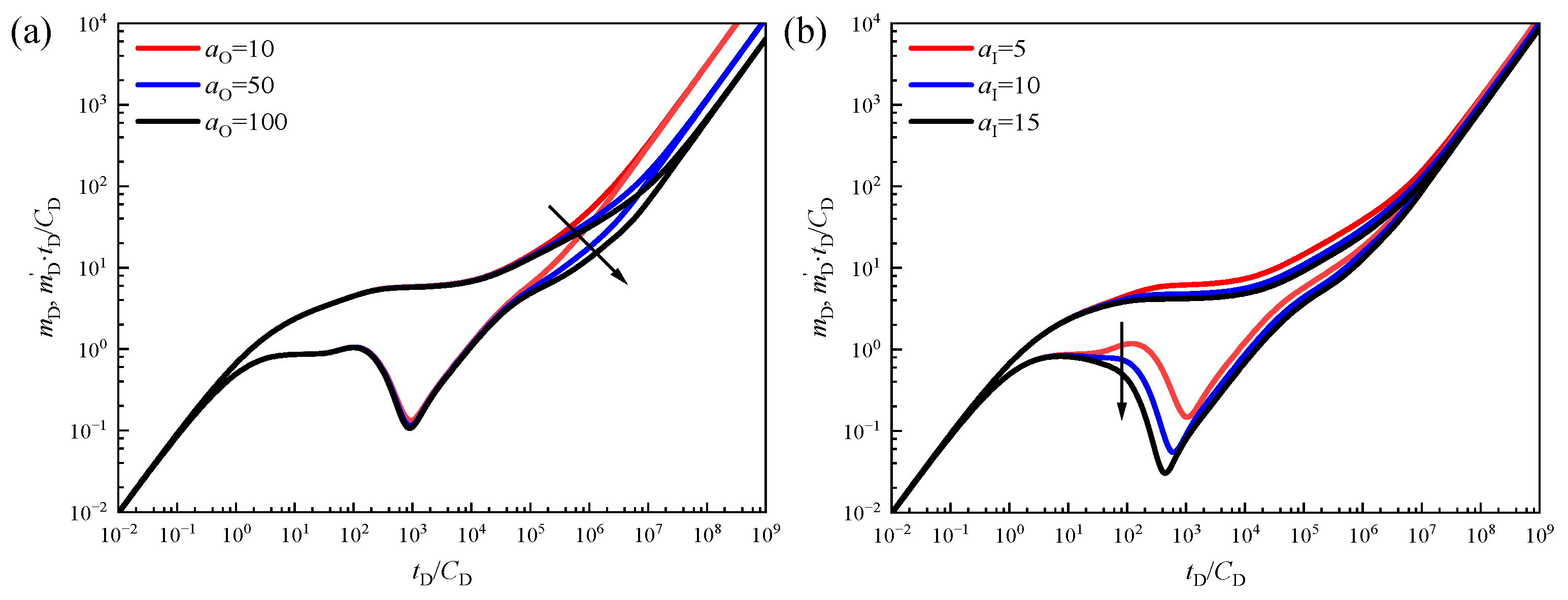
3.3.1. Desorption Coefficient

Figure 5 illustrates the significant impact of the desorption coefficients in the inner and outer regions on each stage of the shale gas flow model. Specifically, the inner region desorption coefficient primarily affects Stage V, the desorption and diffusion stage within the inner matrix system. During this phase, the desorption of adsorbed gas and quasi-steady diffusion of free gas toward the fracture system dominate the flow process. As the inner desorption coefficient increases, the rate of gas desorption accelerates, allowing more gas to desorb from the matrix and diffuse into the fracture system in a shorter amount of time. This is reflected in the increased concavity of the dimensionless pressure derivative curve, which indicates intensified gas migration during desorption and enhanced fluid interaction between the matrix and fracture system.

Similarly, the desorption coefficient in the outer region primarily affects Stage VI, the desorption and diffusion stage in the outer matrix system. Desorption and diffusion remain dominant in the outer matrix, yet the diffusion rate is relatively slower due to the greater distance from the fractures. A higher desorption coefficient increases the desorption rate of gas in the outer region, which manifests as a deeper concavity in the pressure derivative curve. Conversely, when the desorption coefficient in the outer region is low, the desorption process weakens, the diffusion effect is less pronounced, and the concave section of the dimensionless pressure derivative curve becomes shallower and narrower.

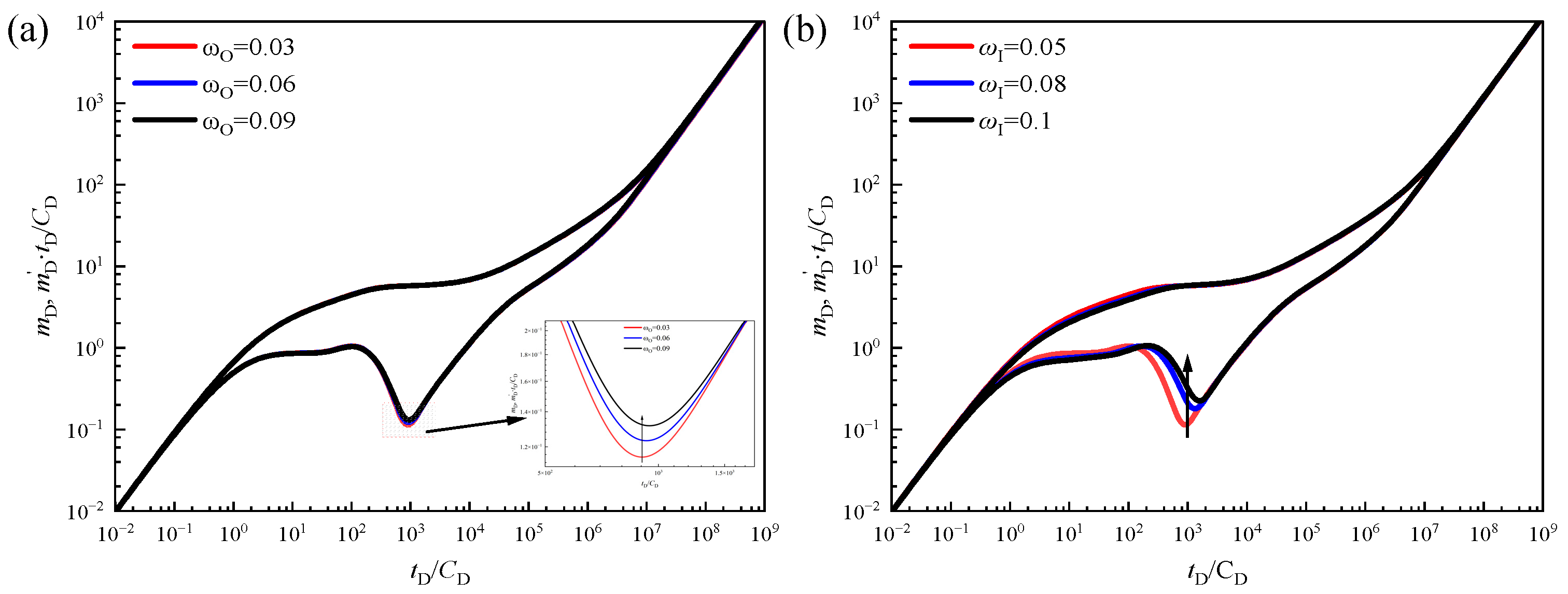
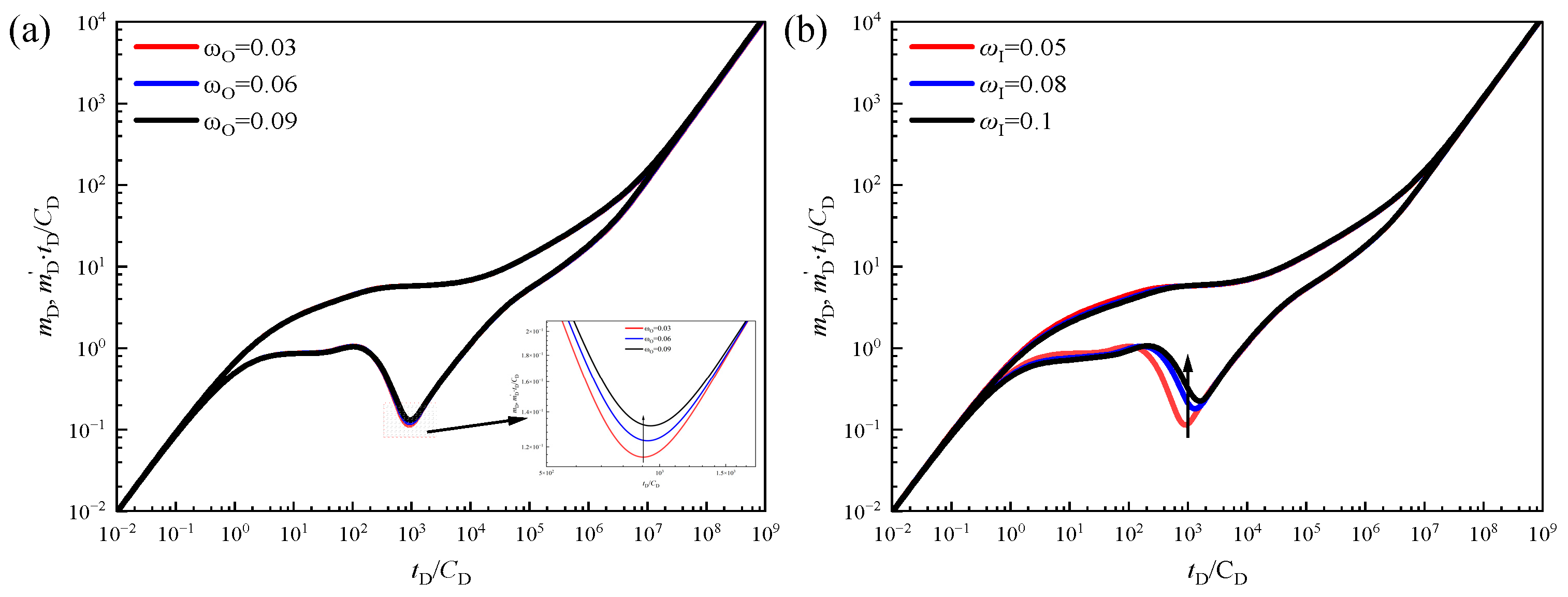
3.3.2. Elastic Storage Ratio

The elastic storage ratio in the inner region is a critical parameter influencing the gas flow characteristics in shale gas reservoirs, particularly affecting the desorption and diffusion stage within the inner region. Physically, a larger elastic storage ratio implies that microfractures in the inner region contribute more to the total storage capacity, enabling them to store more gas. This enhances the gas supply from the matrix to the fracture system, thereby affecting the characteristic features of the pressure derivative curve. As shown in Figure 6, an increase in the elastic storage ratio intensifies the contribution of microfractures to gas flow, accelerating gas accumulation in fractures. With increased gas storage, the pressure drop becomes more gradual, which is reflected by a shallower, narrower concave section on the dimensionless pressure derivative curve. This phenomenon suggests that, during the inner desorption and diffusion stage, flow resistance decreases, allowing the fracture system to more effectively receive and transport gas to the production well.

Compared to the inner region, the outer matrix’s storage capacity contributes less to the overall system, making its influence on the dimensionless pressure response curve less significant. Due to the longer flow path and smaller storage capacity in the outer region, gas diffusion toward the fracture system occurs more slowly, resulting in a weaker pressure response. As illustrated in Figure 6a, changes in outer matrix storage have a limited effect on the overall pressure derivative curve and do not exhibit distinct characteristic features.

3.3.3. Inter-Porosity Coefficients

Figure 7 demonstrates the significant influence of the inter-porosity coefficients in the outer region on shale gas flow characteristics. As the inter-porosity coefficient in the outer region increases, the desorption process begins earlier, indicating that fluids in the outer matrix start diffusing into the fracture system sooner. A higher inter-porosity coefficient strengthens fluid exchange between the matrix and fractures, allowing gas in the matrix to enter the fracture system more quickly. This effect is shown by the earlier appearance of the concave section on the dimensionless pressure derivative curve.

The inter-porosity coefficient in the inner region similarly affects the desorption and diffusion process. With an increase in the inner inter-porosity coefficient, fluid in the inner matrix diffuses into the fracture system earlier. This is reflected by the concave section in the dimensionless pressure derivative curve appearing sooner, indicating that the fluid exchange rate between the inner matrix and fractures accelerates as the inter-porosity coefficient increases. When the inter-porosity coefficient in the inner region exceeds a certain value, flow characteristics change substantially. Particularly in the reservoir linear flow stage, the duration of this stage shortens markedly and may even disappear as the inter-porosity coefficient further increases. This suggests that a high inter-porosity coefficient significantly enhances flow between fractures and the matrix, causing the system to bypass the typical reservoir linear flow stage and directly transition into diffusion-controlled flow.

4. Conclusions

This study established a trilinear flow model for a fractured horizontal shale gas well, incorporating adsorption–desorption and diffusion mechanisms. Using Laplace transformation, Duhamel’s principle, and the Stehfest numerical inversion method, we obtained a dimensionless bottom-hole pressure solution that accounts for wellbore storage and skin effects. Pressure response characteristic curves were generated, the flow stages of the shale gas trilinear flow model were delineated, and the effects of sensitivity parameters, including the desorption coefficient, inter-porosity coefficient, desorption coefficient, and elastic storage ratio, on the pressure response curve were analyzed. Moreover, a Monte Carlo simulation was employed in a pressure transient analysis, thereby offering valuable insights into the uncertainty.

Based on the pressure and pressure derivative response curves, seven distinct flow regimes were identified: the wellbore storage phase, the transitional stage following the wellbore storage, the bilinear flow phase, the formation linear flow phase, the inner region desorption and diffusion phase, the outer region desorption and diffusion phase, and the pseudo-steady-state flow phase of the entire system. The results of the Monte Carlo simulation highlight the variability in the pressure response under different input parameters within the shale gas trilinear flow model. In contrast to single-parameter scenarios, the Monte Carlo simulation provided a more accurate reflection of the model’s behavior in complex environments, as well as the potential impact of varying input conditions on the output.

The sensitivity parameters, including the inter-porosity coefficient, desorption coefficient, and elastic storage ratio, significantly impacted the pressure response characteristic curves. The magnitude of the desorption coefficient directly influenced the rate at which adsorbed gas converted to free gas, thereby controlling the overall rate of gas migration from the matrix to the fracture system in shale reservoirs. In the dimensionless pressure derivative curve, a deeper concave indicated a more pronounced contribution of the desorption process to the overall flow in the reservoir. An increase in the elastic storage ratio amplified the gas contribution from microfractures, accelerating gas accumulation within fractures, which resulted in a gentler pressure drop. This effect was reflected in the dimensionless pressure derivative curve as a shallower, narrower concave section. A higher inter-porosity coefficient enhanced fluid exchange between the matrix and fractures, allowing gas to enter the fracture system more rapidly, causing the concave section of the dimensionless pressure derivative curve to appear earlier.

References

1. Javadpour, F.; Ettehadtavakkol, A. Gas Transport Processes in Shale. In Fundamentals of Gas Shale Reservoirs; John Wiley & Sons, Ltd.: Hoboken, NJ, USA, 2015; pp. 245–266. ISBN 978-1-119-03922-8. [Google Scholar]
2. Yucel Akkutlu, I.; Fathi, E. Multiscale Gas Transport in Shales with Local Kerogen Heterogeneities. SPE J. 2012, 17, 1002–1011. [Google Scholar] [CrossRef]
3. Wang, W.; Fan, D.; Sheng, G.; Chen, Z.; Su, Y. A Review of Analytical and Semi-Analytical Fluid Flow Models for Ultra-Tight Hydrocarbon Reservoirs. Fuel 2019, 256, 115737. [Google Scholar] [CrossRef]
4. Moghanloo, R.G.; Yuan, B.; Ingrahama, N.; Krampf, E.; Arrowooda, J.; Dadmohammadi, Y. Applying Macroscopic Material Balance to Evaluate Interplay between Dynamic Drainage Volume and Well Performance in Tight Formations. J. Nat. Gas Sci. Eng. 2015, 27, 466–478. [Google Scholar] [CrossRef]
5. Lee, S.-T.; Brockenbrough, J.R. A New Approximate Analytic Solution for Finite-Conductivity Vertical Fractures. SPE Form. Eval. 1986, 1, 75–88. [Google Scholar] [CrossRef]
6. Ozkan, E.; Raghavan, R.; Apaydin, O.G. Modeling of Fluid Transfer from Shale Matrix to Fracture Network. In Proceedings of the SPE Annual Technical Conference and Exhibition, Florence, Italy, 20–22 September 2010; OnePetro: Richardson, TX, USA, 2010. [Google Scholar]
7. Brown, M.; Ozkan, E.; Raghavan, R.; Kazemi, H. Practical Solutions for Pressure-Transient Responses of Fractured Horizontal Wells in Unconventional Shale Reservoirs. SPE Reserv. Eval. Eng. 2011, 14, 663–676. [Google Scholar] [CrossRef]
8. Stalgorova, E.; Mattar, L. Analytical Model for Unconventional Multifractured Composite Systems. SPE Reserv. Eval. Eng. 2013, 16, 246–256. [Google Scholar] [CrossRef]
9. Stalgorova, E.; Mattar, L. Practical Analytical Model to Simulate Production of Horizontal Wells with Branch Fractures. In Proceedings of the SPE Canadian Unconventional Resources Conference, Calgary, AB, Canada, 30 October–1 November 2012; OnePetro: Richardson, TX, USA, 2012. [Google Scholar]
10. Haeri, F.; Izadi, M.; Zeidouni, M. Unconventional Multi-Fractured Analytical Solution Using Dual Porosity Model. J. Nat. Gas Sci. Eng. 2017, 45, 230–242. [Google Scholar] [CrossRef]
11. Stalgorova, E.; Mattar, L.; Zhang, J.; Huang, S.; Cheng, L.; Xu, W.; Liu, H.; Yang, Y.; Xue, Y. Effect of Flow Mechanism with Multi-Nonlinearity on Production of Shale Gas. J. Nat. Gas Sci. Eng. 2015, 24, 291–301. [Google Scholar] [CrossRef]
12. Deng, Q.; Nie, R.-S.; Jia, Y.-L.; Huang, X.-Y.; Li, J.-M.; Li, H.-K. A New Analytical Model for Non-Uniformly Distributed Multi-Fractured System in Shale Gas Reservoirs. J. Nat. Gas Sci. Eng. 2015, 27, 719–737. [Google Scholar] [CrossRef]
13. Zhang, L.; Gao, J.; Hu, S.; Guo, J.; Liu, Q. Five-Region Flow Model for MFHWs in Dual Porous Shale Gas Reservoirs. J. Nat. Gas Sci. Eng. 2016, 33, 1316–1323. [Google Scholar] [CrossRef]
14. Zeng, J.; Wang, X.; Guo, J.; Zeng, F. Analytical Model for Multi-Fractured Horizontal Wells in Tight Sand Reservoir with Threshold Pressure Gradient. In Proceedings of the SPE Asia Pacific Hydraulic Fracturing Conference, Beijing, China, 24–26 August 2016; OnePetro: Richardson, TX, USA, 2016. [Google Scholar]
15. Zeng, J.; Wang, X.; Guo, J.; Zeng, F. Composite Linear Flow Model for Multi-Fractured Horizontal Wells in Heterogeneous Shale Reservoir. J. Nat. Gas Sci. Eng. 2017, 38, 527–548. [Google Scholar] [CrossRef]
16. Zhao, K.; Du, P. Performance of Horizontal Wells in Composite Tight Gas Reservoirs Considering Stress Sensitivity. Adv. Geo-Energ. Res. 2019, 3, 287–303. [Google Scholar] [CrossRef]
17. Zhao, K.; Du, P. A New Production Prediction Model for Multistage Fractured Horizontal Well in Tight Oil Reservoirs. Adv. Geo-Energy Res. 2020, 4, 152–161. [Google Scholar] [CrossRef]
18. Wang, Z.; Zhang, L.; Zhang, R.; Wang, R.; Huang, R. Flow Mechanism and Transient Pressure Analysis of Multi-Stage Fractured Horizontal Well. Chem Technol Fuels Oils 2022, 57, 941–954. [Google Scholar] [CrossRef]
19. Guo, T.; Kou, Z.; Zhao, Y.; Wang, H.; Xin, Y. Role of Gas Multiple Transport Mechanisms and Fracture Network Heterogeneity on the Performance of Hydraulic Fractured Multiwell-Pad in Unconventional Reservoirs. Fuel 2023, 342, 127808. [Google Scholar] [CrossRef]
20. Qin, J.-Z.; Zhong, Q.-H.; Tang, Y.; Yu, W.; Sepehrnoori, K. Well Interference Evaluation Considering Complex Fracture Networks through Pressure and Rate Transient Analysis in Unconventional Reservoirs. Pet. Sci. 2023, 20, 337–349. [Google Scholar] [CrossRef]
21. Liang, Y.-Z.; Teng, B.-L.; Luo, W.-J. Study of the Pressure Transient Behavior of Directional Wells Considering the Effect of Non-Uniform Flux Distribution. Pet. Sci. 2024, 21, 1765–1779. [Google Scholar] [CrossRef]
22. Wang, H.; Chen, L.; Qu, Z.; Yin, Y.; Kang, Q.; Yu, B.; Tao, W.-Q. Modeling of Multi-Scale Transport Phenomena in Shale Gas Production—A Critical Review. Appl. Energy 2020, 262, 114575. [Google Scholar] [CrossRef]
23. Moghadam, S.; Mattar, L.; Pooladi-Darvish, M. Dual Porosity Typecurves for Shale Gas Reservoirs. In Proceedings of the Canadian Unconventional Resources and International Petroleum Conference, Calgary, AB, Canada, 19–21 October 2010; OnePetro: Richardson, TX, USA, 2010. [Google Scholar]
Figure 1. Physical model of trilinear flow for fractured horizontal well in shale gas reservoir.
Processes 12 02652 g001
Figure 2. Flowchart of pressure transient analysis for fractured shale gas wells using trilinear flow model. (a) Model pre−processing: Dimensionless variables are defined, physical continuity across the three flow regions is analyzed, and a mathematical model is established, followed by Laplace transformation. (b) The model is solved in the Laplace domain, and inverse transformation is applied to retrieve solutions in the real space domain. (c) The forward model is employed to perform Monte Carlo simulations, enabling quantification of input parameter uncertainties and comprehensive sensitivity analysis.
Processes 12 02652 g002
Figure 3. (a) A comparison of the pressure response characteristic curves of a trilinear flow model for a shale gas, dual − medium, multi − stage fracturing horizontal well and a trilinear flow model for non-desorption diffusion flow; (b) Flow regime division: Stage I: Wellbore storage stage; Stage II: Transition Stage Post-Wellbore Storage; Stage III: Bilinear Flow Between Fractures and Reservoir; Stage IV: Reservoir Linear Flow Stage; Stage V: Desorption and Diffusion Processes in Inner Region Matrix System; Stage VI: Desorption and Diffusion Processes in Outer Region Matrix System; Stage VII: Pseudo-steady-state flow stage of the entire system.
Processes 12 02652 g003
Figure 4. Uncertainty analysis of pressure transients using Monte Carlo simulations.
Processes 12 02652 g004
Figure 5. Effect of desorption coefficients on pressure response characteristic curves: (a) desorption coefficients in outer zone; (b) desorption coefficients in inner zone.
Processes 12 02652 g005
Figure 6. Effect of elastic storage ratio on pressure response characteristic curves: (a) elastic storage ratio in outer zone; (b) elastic storage ratio in inner zone.
Processes 12 02652 g006
Figure 7. Effect of channeling coefficient on pressure response characteristic curves: (a) channeling coefficient in outer zone; (b) channeling coefficient in inner zone.
Processes 12 02652 g007