Advanced Emission Reduction Strategies: Integrating SSSC and Carbon Trading in Power Systems

Abstract

The global power sector faces the critical challenge of balancing rising electricity demand with stringent carbon reduction targets. Taiwan’s unique geopolitical and energy import constraints provide an ideal context for exploring advanced grid technologies integrated with carbon-trading mechanisms. This study combines the Adaptive Time-Varying Gravitational Search Algorithm (ATGA) with Static Synchronous Series Compensator (SSSC) technology to optimize power flow and enable carbon transactions between the power generation and transmission sectors. Through a feedback-driven mechanism, power producers acquire carbon credits from transmission operators, maximizing profitability while meeting emission targets. Managed by the transmission companies, the SSSC enhances grid stability, reduces transmission losses, and generates valuable carbon credits. Simulations based on Taiwan’s power market demonstrate that this integrated approach achieves a 50% reduction in emissions and increases profitability for power producers by up to 20%. This model has potential applications in other regions, and future work could explore its scalability and adaptability in different economic and regulatory contexts.

1. Introduction

Climate change poses a significant global challenge, particularly as the power sector remains a leading source of greenhouse gas emissions, accounting for roughly 42% of global carbon output. In pursuit of carbon neutrality, integrating advanced grid technologies with market-based solutions has become essential [1]. Such innovations not only support local carbon targets but also provide scalable solutions for global sustainability and economic security [2].

The Static Synchronous Series Compensator (SSSC), a Flexible AC Transmission System (FACTS) device, enhances grid stability and power flow. While SSSC and carbon-trading mechanisms are well studied separately, their integration offers dual benefits in grid reliability and emissions reduction. SSSC reduces energy losses, improves power quality, and supports renewable energy integration [3]. This not only helps address the mismatch between electricity supply and demand but also reduces transmission losses, thereby offering potential emissions reduction benefits. However, the effective deployment of these technologies requires sophisticated optimization algorithms to manage challenges such as load flow, dynamic dispatch, and emission control. By precisely controlling power flow, the SSSC helps mitigate the mismatch between energy supply and demand caused by the inherent variability of renewable resources [4,5].

In parallel, the rise of carbon-trading mechanisms offers a market-driven approach to reducing emissions, with notable successes in established markets like the European Union’s Emissions Trading System (EU ETS) [6]. For example, the EU ETS has successfully reduced greenhouse gas emissions by more than 30% since its inception in 2005, while also incentivizing investments in renewable energy [7]. For energy-dependent economies like Taiwan, although facing several constraints [8,9], these successful experiences provide valuable insights for developing local carbon trading policies suited to Taiwan’s unique circumstances. Taiwan, with its heavy dependence on energy imports, encounters distinct challenges in its pursuit of energy transition. Due to its geopolitical constraints, Taiwan is excluded from major international climate agreements like the Paris Agreement, which significantly limits its involvement in global climate governance [10]. Despite these challenges, Taiwan has developed domestic carbon trading initiatives aimed at achieving its emissions reduction targets for 2030. Taiwan’s carbon-trading policies have encouraged investments in renewable energy, gradually decreasing the island’s dependence on fossil fuels and shifting its energy structure toward a more sustainable future [11].

Although a growing body of research on grid technologies and carbon-trading mechanisms exists, systematic studies integrating these two fields to achieve both grid stability and emissions reduction are still limited. Much of the existing literature explores the individual impacts of FACTS devices, including the SSSC, on power systems. However, studies specifically examining the combined use of SSSC technology and carbon-trading mechanisms for optimizing both economic dispatch and emissions control are scarce [12,13]. This paper addresses this gap by developing a novel model that integrates SSSC technology with adaptive, market-driven carbon strategies to enhance power flow efficiency and meet emission targets, particularly in constrained power markets like Taiwan’s. However, there is a notable gap in how these technologies can be synergized with carbon trading to improve grid reliability and maximize emissions reductions. To address this gap, advanced optimization algorithms are necessary to manage the complex dynamics of power flow and emissions reduction. To achieve the optimal integration of SSSC and carbon-trading mechanisms, advanced optimization algorithms are crucial to managing the complex dynamics of power flow and emissions reductions. For instance, Zhang et al. (2024) highlighted the potential of the SSSC in dynamic economic dispatch (DED), showing that this approach can significantly enhance system flexibility and responsiveness, resulting in more efficient emissions reduction [14]. Similarly, Hong et al. (2022) emphasized the critical role of grid technology in emissions reduction, particularly in supporting the integration of renewable energy and optimizing power flows [15].

Recent studies on low-carbon economic dispatch and locational marginal electricity-carbon pricing demonstrate the effectiveness of carbon trading in improving energy efficiency [16,17]. However, a significant theoretical gap exists in the integration of carbon-trading mechanisms with advanced grid technologies, specifically with the SSSC, to enhance grid reliability and achieve substantial emissions reduction. This paper addresses this gap by proposing an innovative framework that combines carbon market-driven strategies with emerging grid technologies. Through this integration, the study seeks to advance both theoretical and practical insights into optimizing energy efficiency and emissions reductions in power systems, showcasing the potential for a more resilient, low-carbon grid.

By combining the technical capabilities of the SSSC with market-based carbon pricing strategies, Taiwan can better achieve its dual goals of economic growth and environmental sustainability. Similarly, the SSSC has shown the potential to enhance the effectiveness of emissions reduction policies when deployed within renewable energy systems [18,19]. However, more empirical studies are needed to explore the practical applications of this integration, especially in regions like Taiwan, where energy security concerns and geopolitical constraints are critical [20,21].

Metaheuristic algorithms like PSO and GA address load flow and dispatch optimization, but integrating carbon emissions and renewable energy improves multi-objective capabilities. Studies, including Wang et al. [22] and Fang et al. [23], demonstrate the potential of advanced algorithms like the improved gravitational search algorithm (IGSA) [24] to balance efficiency and solution quality. Optimization algorithms are crucial for integrating the SSSC and carbon trading to achieve reliability, economic dispatch, and emissions reduction.

Building on these advancements, this study addresses the remaining gaps by applying an integrated approach to carbon trading and power dispatch. This combination offers a scalable solution for constrained energy markets, enhancing both economic efficiency and environmental sustainability. Specifically, most studies have concentrated on either optimizing the load flow [25] or minimizing emissions [26]. Few have explored the simultaneous optimization of power system reliability, economic dispatch, and carbon trading, as seen in studies focusing on dynamic economic dispatch with integrated renewable energy and demand-side management [27] or robust low-carbon economic dispatch under renewable uncertainty [28]. This research aims to fill this gap by applying an Adaptive Time-Varying Gravitational Search Algorithm (ATGA) in combination with SSSC technology, which enhances both power flow efficiency and emissions reduction in the context of carbon trading.

Although several algorithms have been successfully applied to improve economic dispatch and minimize emissions, integrating these methods with carbon-trading mechanisms remains underexplored, particularly in constrained environments like Taiwan’s power market [29,30]. This study expands upon the existing research by addressing the gap in simultaneously optimizing power flow and emissions through the integration of SSSC technology with carbon-trading mechanisms. This innovative combination demonstrates how advanced grid technologies can enhance power system reliability and achieve substantial emissions reduction, offering a scalable model for other regions.

The ATGA demonstrates how integrating SSSC technology with a dynamic carbon market enhances power system resilience and economic viability. For Taiwan, adopting the SSSC can reduce power losses and improve renewable energy integration, supporting carbon reduction goals [29,31]. Further research should explore flexible grid technologies and their interaction with carbon trading to build adaptive energy systems. Studies on decoupling economic growth from emissions [32] and integrating multi-energy systems [33] underscore the importance of grid flexibility in achieving carbon reduction.

In summary, while significant research has been conducted on both carbon trading and grid technologies, the intersection of these fields remains underexplored. This paper aims to address this gap by investigating the integration of SSSC technology with carbon-trading mechanisms and dynamic economic dispatch in Taiwan’s power market. By doing so, this research seeks to provide practical solutions for Taiwan and other regions facing similar challenges, thereby contributing to the broader goal of global energy transition and sustainable development. While traditional emissions-reduction technologies focus on direct carbon output mitigation, this study’s market-based approach aims to address emissions reduction through policy-driven incentives. This approach reflects a distinct focus on creating a financially viable and sustainable mechanism that can be adapted to regions like Taiwan, where a formal carbon-trading market does not yet exist. This focus on policy and market mechanisms differentiates it from engineering-based carbon-reduction technologies. Future research could explore the scalability of this model in regions with different economic and regulatory conditions, ensuring its broader applicability and transferability.

2. Global Carbon-Trading Mechanisms: Evolution and Key Drivers

2.1. Evolution and Drivers of Global Carbon-Trading Mechanisms

As climate change intensifies, nations have increasingly adopted carbon-trading mechanisms to curb greenhouse gas emissions. Carbon trading, which caps emissions and allows the trading of emission permits, has emerged as a central policy tool in this effort. The European Union’s Emissions Trading System (EU ETS), launched in 2005, set a benchmark for other regions by demonstrating the efficacy of market-based solutions [20].

The key driver of carbon trading is the economic incentive it provides. Companies can buy or sell carbon permits based on their ability to meet emissions reduction targets, fostering flexibility and efficiency in achieving compliance. Article [6] of the Paris Agreement further promotes global cooperation by enabling countries to collaborate on emissions reduction efforts, offering a more flexible and cost-effective pathway to achieving global targets. Taiwan, however, faces significant barriers to participation in these global carbon markets due to its political status [34]. As a result, Taiwan must innovate domestically and develop market-based solutions to meet its emissions reduction goals. This study explores how integrating carbon trading with power dispatch optimization offers a viable pathway for Taiwan to balance economic growth with effective carbon management.

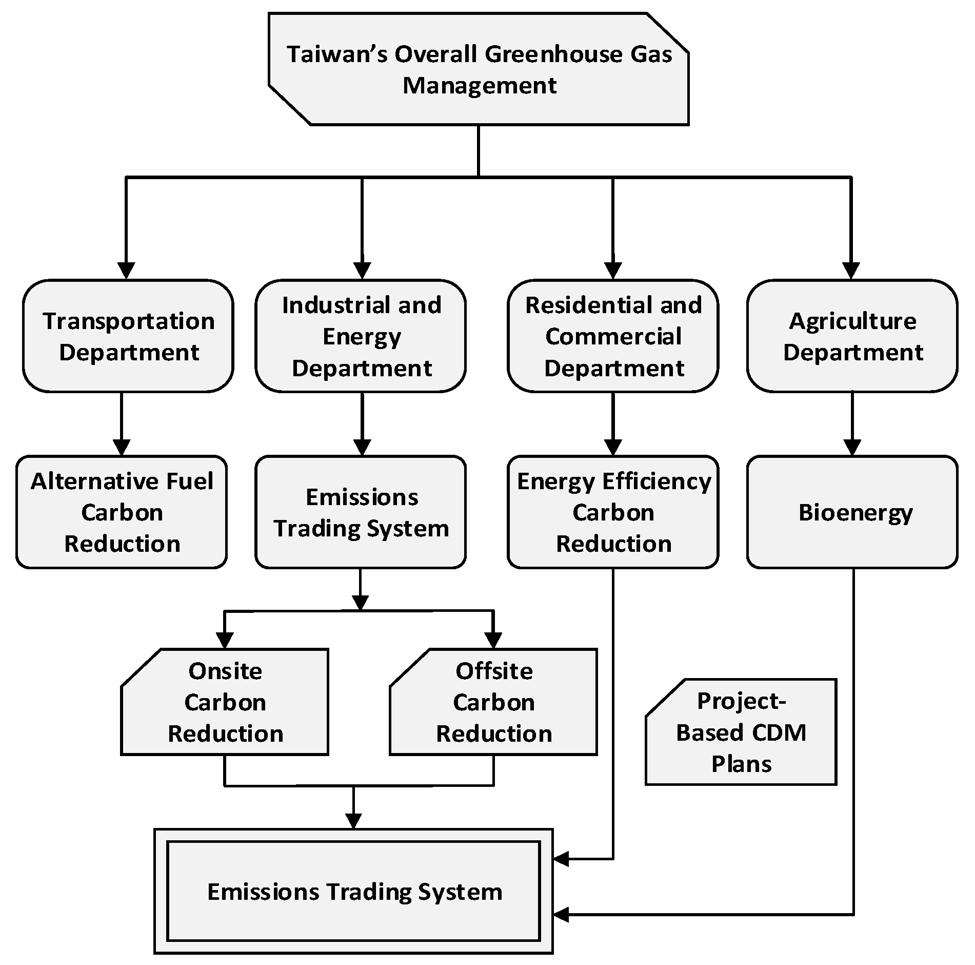
2.2. Taiwan’s Carbon-Trading System and Market Challenges

Taiwan faces significant challenges in establishing a carbon-trading system, primarily due to its exclusion from international agreements like the Paris Agreement. Unlike well-established markets such as the EU ETS, Taiwan’s framework relies on domestic policy adaptations without the advantage of international linkages. This study’s focus on a localized market-driven approach contrasts with the operational scope of other mature carbon markets, offering insights into the development of emissions reduction strategies for regions with emerging carbon policies. By proposing an adaptable, region-specific mechanism, this research contributes to a broader understanding of how market-based approaches can be customized in various policy contexts. As a result, Taiwan must rely on domestic policies, such as the Greenhouse Gas Reduction and Management Act, to implement cap-and-trade systems aimed at reducing emissions in high-emission sectors, particularly power generation and manufacturing.

Taiwan’s limited industrial and energy sectors create cost-effectiveness challenges for its carbon-trading system. Expanding participation to sectors like transportation (alternative fuels), commercial (energy efficiency), and agriculture (afforestation and bioenergy) could enhance market liquidity and efficiency. Figure 1 presents a framework for broader participation to increase emissions reduction potential and address the constraints of smaller sectors.

Compared with larger international markets with greater liquidity, Taiwan faces significant challenges in scaling its carbon market. Linking to voluntary systems, such as California’s cap-and-trade program, could help Taiwanese industries gain experience and prepare for future global market participation.

Technological advancements are essential for the success of Taiwan’s carbon-trading system. By adopting grid-optimization technologies such as SSSC and promoting renewable energy deployment, Taiwan can simultaneously improve energy efficiency and reduce emissions. These innovations will create additional carbon credits, enhancing the market’s scalability and fostering a dynamic, more effective carbon-trading system.

2.3. Power Market Dynamics

The global trend toward power market liberalization is accelerating, driven by increased economic interdependence and competition following the establishment of institutions such as the General Agreement on Tariffs and Trade (GATT) and the World Trade Organization (WTO). The core goal of this liberalization is to enhance the efficiency of power generation and transmission through competitive market mechanisms, reduce electricity prices, and encourage the widespread adoption of renewable energy sources. In Taiwan, power market reform is both a challenge and an opportunity, particularly within the context of carbon trading and emissions control. Market liberalization can play a crucial role in supporting Taiwan’s efforts to achieve carbon neutrality.

Traditionally, power systems relied on cost-based mechanisms to dispatch generation. With market liberalization, Taiwan is transitioning to competitive bidding, where advanced dispatch technologies like the SSSC improve grid efficiency, reduce losses, and lower emissions. Market liberalization supports resource optimization and a robust carbon-trading system. In Taiwan, combining dynamic economic dispatch (DED) with carbon trading enhances emissions control, while market opening incentivizes clean energy use and emissions reduction through additional revenues.

By integrating SSSC technology with dynamic economic dispatch models, Taiwan can optimize grid operations and reduce emissions from power generation without compromising electricity supply reliability. Power market liberalization improves overall generation efficiency, promotes the use of renewable energy, and supports Taiwan’s broader carbon reduction goals. Similar to the modeling techniques used in high-resolution environmental data monitoring networks, as discussed by Sofia et al. (2018), this approach also benefits from the integration of detailed environmental data for better emissions management and grid optimization [35].

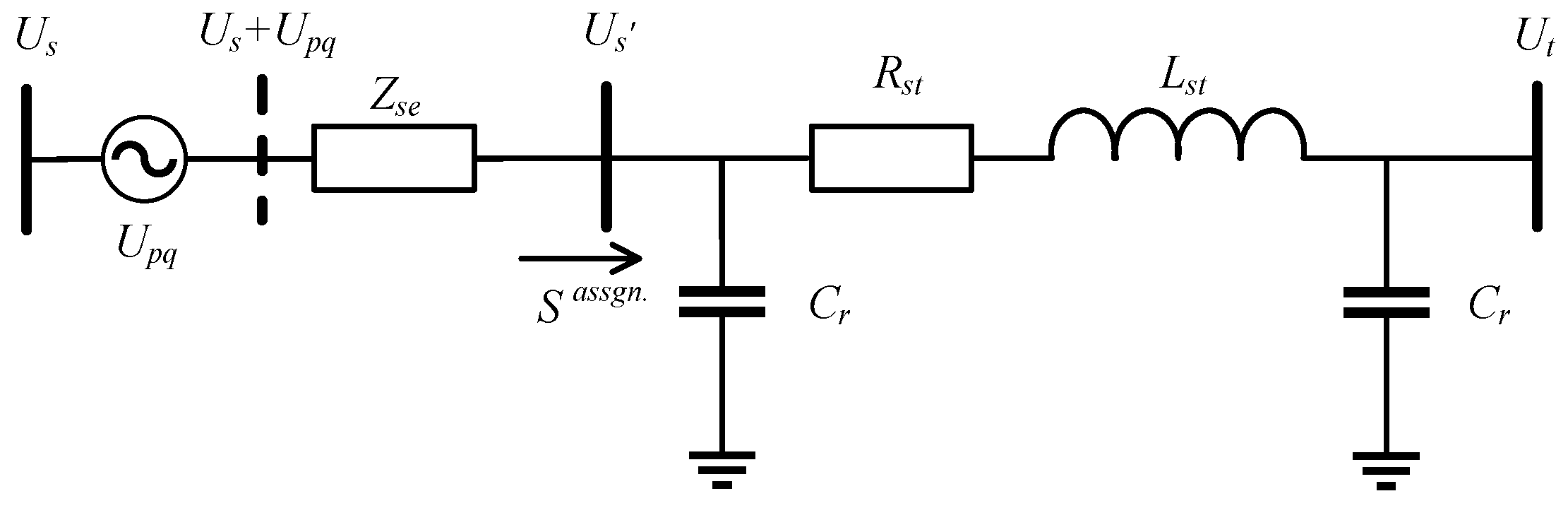
3. Integration of the SSSC into the Power Market Load Flow Model

As power markets liberalize, grid complexity increases, requiring technologies like SSSCs for optimization and emission control. The SSSC minimizes losses, enhances transmission, and reduces carbon costs, enabling producers to lower purchases and operators to earn rebates. The equivalent current injection (ECI) method, effective for unbalanced systems [31], has been enhanced with a robust, efficient decoupling model for high-voltage transmission.

3.1. Power Flow Calculation Using the ECI Approach

The equivalent current injection method, effective in three-phase unbalanced systems, is combined with the Newton–Raphson method for fast convergence and stability to address load flow in transmission systems and develop a mathematical model.

A transmission line between buses m and n is modeled using a π representation (Figure 2), with resistance R_mn, inductance L_mn, and admittance G_mn + jB_mn. Line capacitance C_r corresponds to a susceptance of jB_c, defining the equivalent current injection at bus m [31].

$$I_m\left(t\right)={\displaystyle \frac{-S_m}{U_m{\left(t\right)}^{*}}}=I_m^{\left(r\right)}\left(t\right)+j{I}_m^{\left(i\right)}\left(t\right)$$

(1)

In this scenario, S_m indicates the complex power being injected at bus m, while U_m represents the corresponding terminal voltage at that bus. The superscript t denotes the current iteration step, with the superscripts (r) and (i) indicating the real and imaginary parts of the values, respectively.

The currents I_m and I_n injected at buses m and n can be expressed in rectangular coordinate format as follows:

$$I_m=\left[G_{mn}\left(U_m^{\left(r\right)}-U_n^{\left(r\right)}\right)-B_{mn}\left(U_m^{\left(i\right)}-U_n^{\left(i\right)}\right)-B_c{U}_m^{\left(i\right)}\right]+j\left[G_{mn}\left(U_m^{\left(i\right)}-U_n^{\left(i\right)}\right)-B_{mn}\left(U_m^{\left(r\right)}-U_n^{\left(r\right)}\right)+B_c{U}_m^{\left(r\right)}\right]$$

(2)

$$I_n=\left[G_{mn}\left(U_n^{\left(r\right)}-U_m^{\left(r\right)}\right)-B_{mn}\left(U_n^{\left(i\right)}-U_m^{\left(i\right)}\right)-B_c{U}_n^{\left(i\right)}\right]+j\left[G_{mn}\left(U_n^{\left(i\right)}-U_m^{\left(i\right)}\right)-B_{mn}\left(U_n^{\left(r\right)}-U_m^{\left(r\right)}\right)+B_c{U}_n^{\left(r\right)}\right]$$

(3)

Afterward, I_m and I_n should be divided into their real and imaginary components. Equations (1)–(3) can then be reformulated in the context of the Newton–Raphson method, resulting in

$$\left[\begin{array}{c}\Delta I^{\left(r\right)}\left(t\right)\\ \Delta I^{\left(i\right)}\left(t\right)\end{array}\right]=\left[\begin{array}{cc}{\displaystyle \frac{\partial I^{\left(r\right)}}{\partial U^{\left(r\right)}}}& {\displaystyle \frac{\partial I^{\left(r\right)}}{\partial U^{\left(i\right)}}}\\ {\displaystyle \frac{\partial I^{\left(i\right)}}{\partial U^{\left(r\right)}}}& {\displaystyle \frac{\partial I^{\left(i\right)}}{\partial U^{\left(i\right)}}}\end{array}\right]\left[\begin{array}{c}\Delta U^{\left(r\right)}\\ \Delta U^{\left(i\right)}\end{array}\right]$$

(4)

Here, ∆I_r refers to the real component of the difference between the specified equivalent current injection and the calculated current. Similarly, ∆I⁽ⁱ⁾ denotes the imaginary component of this difference between the expected equivalent injected current and the computed current value. For Equations (2) and (3), the partial derivatives should be taken concerning the state variables $U_m^{\left(r\right)}$, $U_m^{\left(i\right)}$, $U_n^{\left(r\right)}$, and $U_n^{\left(i\right)}$. The organized error equations can then be presented as follows:

$$\left[\begin{array}{c}\Delta I_m^{\left(r\right)}\\ \Delta I_n^{\left(r\right)}\\ \Delta I_m^{\left(i\right)}\\ \Delta I_n^{\left(i\right)}\end{array}\right]=\left[\begin{array}{c}{G}_{mn}\\ -G_{SR}\\ (B_{mn}+B_c)\\ -B_{SR}\end{array}\begin{array}{c}-G_{mn}\\ G_{SR}\\ -B_{SR}\\ (B_{mn}+B_c)\end{array}\begin{array}{c}-\left(B_{mn}+B_C\right)\\ B_{mn}\\ G_{mn}\\ -G_{mn}\end{array}\begin{array}{c}{B}_{mn}\\ -\left(B_{mn}+B_c\right)\\ -G_{mn}\\ G_{mn}\end{array}\right]\left[\begin{array}{c}\Delta U_m^{\left(r\right)}\\ \Delta U_n^{\left(r\right)}\\ \Delta U_m^{\left(i\right)}\\ \Delta U_n^{\left(i\right)}\end{array}\right]=\left[J_{mn}\right]\left[\begin{array}{c}\Delta U^{\left(r\right)}\\ \Delta U^{\left(i\right)}\end{array}\right]$$

(5)

Based on Equation (5), it is apparent that the matrix serves as a Jacobian matrix during the iterative process, with its components corresponding directly to the admittance matrix linking buses m and n. Significantly, all entries in this Jacobian matrix are fixed and are not influenced by the system’s state variables, resulting in a constant Jacobian matrix that is invariant with respect to the state. This principle can be briefly articulated as follows:

$$\left[\begin{array}{c}\Delta I^{\left(r\right)}\left(t\right)\\ \Delta I^{\left(i\right)}\left(t\right)\end{array}\right]=\left[\begin{array}{cc}{y}_G& -y_B\\ y_B& y_G\end{array}\right]\left[\begin{array}{c}\Delta U^{\left(r\right)}\left(t\right)\\ \Delta U^{\left(i\right)}\left(t\right)\end{array}\right]$$

(6)

Generator buses (PV buses), including wind generators, require distinct modeling compared with load buses. Aligning their parameters with traditional load flow models poses challenges, necessitating their integration into the equivalent current injection framework for a complete system model. To overcome the issues related to PV buses in the equivalent current injection method, the real power injected at a PV bus can be expanded using a Taylor series, yielding the following:

$$\Delta P_m=U^{\left(r\right)}·\Delta I_m^{\left(r\right)}.+U^{\left(i\right)}·\Delta I_m^{\left(i\right)}+U^{\left(r\right)}·I_m^{\left(r\right)}+U^{\left(i\right)}·I_m^{\left(i\right)}$$

(7)

By substituting Equation (5) into Equation (7) and reorganizing the terms, Equation (8) is obtained:

$$\begin{gathered} \Delta P_m=\left(U_m^{\left(r\right)}{G}_{mn}+U_m^{\left(i\right)}{B}_{mn}^{\prime }+I_m^{\left(r\right)}\right)\Delta U_m^{\left(r\right)}+\left(-U_m^{\left(r\right)}{B}_{mn}^{\prime }{U}_m^{\left(i\right)}{G}_{mn}+I_m^{\left(i\right)}\right)\Delta U_m^{\left(i\right)} \\ +\left(-U_n^{\left(r\right)}{G}_{mn}{U}_n^{\left(i\right)}{B}_{mn}\right)\Delta U_n^{\left(r\right)}+\left(-U_n^{\left(r\right)}{B}_{mn}{U}_n^{\left(i\right)}{G}_{mn}\right)\Delta U_n^{\left(i\right)} \end{gathered}$$

(8)

where $B_{mn}^{\prime }=B_{mn}+B_c$.

By applying a Taylor series expansion to the generator’s terminal voltage ${\left|U_m\right|}^2={U_m^{\left(r\right)}}^2+{U_m^{\left(i\right)}}^2$, the result can be expressed as follows:

$$\Delta {\left|U_m\right|}^2=2U_m^{\left(r\right)}\Delta U_m^{\left(r\right)}+2U_m^{\left(i\right)}\Delta U_m^{\left(i\right)}$$

(9)

Rearranging Equations (8) and (9) allows for the derivation of the Jacobian matrix for voltage control buses and the corresponding error equation, as shown in Equation (10).

$$\left[\begin{array}{c}\Delta P_m\\ \Delta {\left|U_m\right|}^2\end{array}\right]=\left[\begin{array}{cc}{J}_1& J_2\\ J_3& J_4\end{array}\right]\left[\begin{array}{c}\Delta U_m^{\left(r\right)}\\ \Delta U_m^{\left(i\right)}\\ \Delta U_n^{\left(r\right)}\\ \Delta U_n^{\left(i\right)}\end{array}\right]$$

(10)

where $J_1=\left[\begin{array}{cc}\left(U_m^{\left(r\right)}{G}_{SR}+U_m^{\left(i\right)}{B}_{SR}^{\prime }+I_m^{\left(r\right)}\right)& \left(-U_m^{\left(r\right)}{G}_{SR}-U_m^{\left(i\right)}{B}_{SR}\right)\end{array}\right]$, $J_2=\left[\begin{array}{cc}\left(-U_m^{\left(r\right)}{B}_{SR}^{\prime }+U_m^{\left(i\right)}{G}_{SR}+I_m^{\left(i\right)}\right)& \left(U_m^{\left(r\right)}{B}_{SR}-U_m^{\left(i\right)}{G}_{SR}\right)\end{array}\right]$, $J_3=\left[2U_m^{\left(r\right)} 0\right]$, $J_4=\left[2U_m^{\left(i\right)} 0\right]$.

By applying the above formula, P and U can be calculated and substituted into the left-hand side of Equation (5), resulting in the formulation of a comprehensive load flow error equation, as demonstrated in Equation (10).

$$\left[\begin{array}{c}\Delta I_1^{\left(r\right)}\\ ⋮\\ \Delta P_m\\ ⋮\\ \Delta I_j^{\left(r\right)}\\ ⋮\\ \Delta I_1^{\left(i\right)}\\ ⋮\\ \Delta {\left|U_m\right|}^2\\ ⋮\\ \Delta I_j^{\left(i\right)}\end{array}\right]=\left[\begin{array}{cc}{J}_G^{\left(r\right)}& J_B^{\left(r\right)}\\ J_B^{\left(i\right)}& J_G^{\left(i\right)}\end{array}\right]\left[\begin{array}{c}\Delta U_1^{\left(r\right)}\\ ⋮\\ \Delta U_m^{\left(r\right)}\\ ⋮\\ \Delta U_j^{\left(r\right)}\\ ⋮\\ \Delta U_1^{\left(i\right)}\\ ⋮\\ \Delta {\left|U_m^{\left(i\right)}\right|}^2\\ ⋮\\ \Delta U_j^{\left(i\right)}\end{array}\right]$$

(11)

In a j-bus system with voltage-control buses, the Jacobian matrix requires updates at each iteration for elements related to these buses. However, the adjustments are fewer compared with the standard Newton–Raphson method, as only the voltage control elements are modified.

3.2. Derivation of a ECI Model Incorporating SSSC

The SSSC is a series-connected device that regulates power flow by adjusting line impedance via voltage injection aligned with the line current’s phase. Using a Voltage Source Converter (VSC) and Pulse Width Modulation (PWM), it controls line voltage, reduces losses, and stabilizes the system. Figure 3 shows the SSSC structure, including the energy storage, VSC, and control system [33].

The diagram in Figure 3 has been simplified into the equivalent single-line diagram shown in Figure 4, which represents a common equivalent circuit model for SSSCs in power systems. This model describes the interaction between the SSSC and the transmission line through the impedance Z_se = R_se + jX_se, where R_se represents the active power losses in the coupling transformer and associated components, while X_se reflects the characteristics of the reactive power exchange. To better represent the impact of the SSSC on the transmission system, this model is integrated with the ECI model, allowing for a more precise analysis of voltage and power regulation within the system.

The SSSC is modeled as an equivalent current injection, representing its impact as a complex current I_se injected into the line via the coupling transformer. The magnitude and phase of I_se depend on the impedance Z_se and voltage source U_pq. This approach integrates the SSSC into the ECI framework for unified power flow analysis.

This model in Figure 4 uses a series voltage source to describe the converter behavior of the SSSC. The magnitude of the voltage U_pq and its angle θ_pq are constrained by Equations (12) and (13). In other words, the SSSC’s operation is governed by these limitations, ensuring that the voltage magnitude and phase angle injected by the converter stay within the specified bounds.

$$\underset{¯}{U_{pq}}\le U_{pq}\le \overline{U_{pq}}$$

(12)

$$0\le {\theta }_{pq}\le 2\pi$$

(13)

where $\overline{U_{pq}}$ and $\underset{¯}{U_{pq}}$ denote the maximum and minimum values of the voltage that the SSSC can inject, with the voltage angle θ_pq constrained between 0 and 2π.

In the discussion above, the original voltage source model can be transformed into a current source model via Norton’s theorem, which is the model used in this paper and integrated into the power system, as shown in Figure 5. To simplify the system’s structure, the impedance of the π model and the SSSC are treated separately to facilitate clearer analysis. During the simulation, a virtual bus is inserted between the π model and the SSSC model, through which the active and reactive power on the transmission line is controlled. In other words, the virtual bus allows for control of the real and reactive power by regulating the complex power S^assgn passing through the transmission line.

To facilitate integration with the equivalent current injection approach, the complex power that needs to be controlled can be incorporated into the equations, articulated by Equation (14):

$$I_{s,s\prime }={\displaystyle \frac{S^{assgn.}}{U_{s\prime }}}=\left(U_s+U_{pq}-U_{s\prime }\right)·\left(G_{se}+j{B}_{se}\right)$$

(14)

As the system undergoes changes, the connection between the updated admittance matrix and the equivalent injected current can be outlined in Equation (15):

$$\left[\begin{array}{c}\begin{array}{c}⋮\\ I_s\end{array}\\ ⋮\\ I_{s^{\prime }}\\ ⋮\\ I_{s,s^{\prime }}\end{array}\right]=\left[\begin{array}{c}\cdots \\ \cdots \\ \cdots \\ \cdots \\ \cdots \\ 0\end{array}\begin{array}{c}\cdots \\ \cdots \\ \cdots \\ \cdots \\ \cdots \\ G_{se}+j{B}_{se} \end{array}\begin{array}{c}\cdots \\ \cdots \\ \cdots \\ \cdots \\ \cdots \\ 0\end{array}\begin{array}{c}\cdots \\ \cdots \\ \cdots \\ \cdots \\ \cdots \\ G_{se}+j{B}_{se} \end{array}\begin{array}{c}\cdots \\ \cdots \\ \cdots \\ \cdots \\ \cdots \\ 0\end{array}\begin{array}{c}\cdots \\ G_{se}+j{B}_{se}\\ ⋮\\ -G_{se}-j{B}_{se}\\ ⋮\\ G_{se}+j{B}_{se}\end{array}\right]\left[\begin{array}{c}\begin{array}{c}⋮\\ U_s\end{array}\\ ⋮\\ U_{s\prime }\\ ⋮\\ U_{pq}\end{array}\right]$$

(15)

Here, G_se + jB_se = 1/Z_se by decomposing the voltage and current in Equation (14) into their respective real and imaginary components and updating the new admittance matrix with Equation (6). Integrating the SSSC into the power system enables load flow calculations using the equivalent current injection method to determine system parameters and the voltage source U_pq. Energy injection via the coupling transformer assumes no conversion losses, requiring recalculation of the actual power losses or increments after each iteration. This paper proposes an improved SSSC model that enhances control capabilities and simplifies problem solving through the equivalent current injection method, reducing computational load and meeting real-time monitoring demands.

3.3. Installation Principles of the SSSC

SSSC installation must balance cost and effectiveness, making it a last resort after alternatives like generator dispatch, transformer adjustments, or reactive power solutions prove insufficient.

To maximize the cost-effectiveness of installing the SSSC, certain transmission lines are deemed unsuitable for installation, and these are categorized as follows:

• Each transmission line or bus is limited to one SSSC installation.
  The SSSC regulates power flow, but adding more than one per line offers little benefit and increases reactive power demand, limiting installations to one per line.
• The SSSC should not be installed on lines with significantly low impedance.
  Low-impedance lines naturally carry higher power flow, making rerouting to under-utilized lines more effective than installing the SSSC for congestion reduction.
• Buses with existing generators or synchronous machines are unsuitable for SSSC installation.
  Generators and synchronous machines can address congestion, reducing SSSC need. In Taiwan, separate generation and transmission may still warrant SSSCs for optimization.

3.4. Max Profit Model for Power Generators in Carbon Markets

Considering the combined electricity and carbon-trading markets, the objective is to maximize the profit, represented as follows:

$$\mathrm{Max}\Pi \left(q_{spot}, q_{carbon}\right)=Revenue\left(q_{spot}, q_{carbon}\right)-Cost\left(q_{spot}, q_{carbon}\right)$$

(16)

where $\Pi \left(q_{spot}, q_{carbon}\right)$ represents the profit function with spot power market price ${\mathrm{q}}_{\mathrm{spot}}$ (TWD/MWh) and the carbon market price $q_{carbon}$ (TWD/ton) as inputs.

$$Revenue\left(q_{spot}, q_{carbon}\right)=P_{spot\text{\_}sell}·q_{spot}+E_{carbon\text{\_}sell}·q_{carbon}$$

(17)

$$\begin{gathered} Cost\left(q_{spot}, q_{carbon}\right)=P_{spot\text{\_}buy}·q_{spot}+E_{carbon\text{\_}buy}·q_{carbon} \\ +C_{gen}\left(q_{spot}\right)+C_{trans}\left(q_{spot}\right) \end{gathered}$$

(18)

where $P_{spot\text{\_}sell}$ represents the income from selling power in the power spot market. $E_{carbon\text{\_}sell}$ represents the income from selling carbon allowances in the carbon-trading market. $P_{spot\text{\_}buy}$ represents the expense from buying power in the spot market. $E_{carbon\text{\_}buy}$ represents the expense from buying carbon allowances in the carbon-trading market. $C_{trans}$ represents the transmission fees that power generators are required to pay to transmission operators. $C_{gen}$ is the total generation cost for the power generator, as in (19).

$$C_{gen}\left(P_{g_i}\right)={\displaystyle \sum }_{j\in g_i}^{n_g}{A}_i{P}_{g_i}^2+B_i{P}_{g_i}+C_i$$

(19)

Let $P_{g_i}$ denote the controllable real power from the i-th thermal power unit. The terms $A_i$, $B_i$, and $C_i$ represent the respective cost coefficients linked to the power generation of this plant.

• Equality constraints:

  (1)

  Power balance constraint

The power balance constraint stipulates that the generated power must match the demand in every time interval. Since transmission losses occur, the total generation must equal the sum of the load demand and the transmission losses during each period.

$${\displaystyle \sum }_{i=1}^{n_g}{P}_{g_i}\left(t\right)+P_{d_i}\left(t\right)+P_l=0$$

(20)

Here, $P_{g_i}\left(t\right)$ and $P_{d_i}\left(t\right)$ represent the generation and load demand at bus i during time period t, respectively. $P_l$ represents transmission losses.

• (2)

  OPF equality constraint

The objective of the OPF is to minimize the expression in Equation (19) while satisfying the equality constraints outlined in Equations (21)–(23).

$$-I_{assgn.}+I_{com}=0$$

(21)

$$-P_{assgn.\text{\_}gen}+P_l+P_{com\text{\_}gen}=0$$

(22)

$$-{\left|U_{assgn.}\right|}^2+{\left|U_{com}\right|}^2$$

(23)

where $I_{assgn}=\left[\begin{array}{c}{I}_{assgn.}^{\left(r\right)}\\ I_{assgn.}^{\left(i\right)}\end{array}\right]$ and $I_{com}=\left[\begin{array}{c}{I}_{com}^{\left(r\right)}\\ I_{com}^{\left(i\right)}\end{array}\right]$ are matrices representing the assigned and computed equivalent current injections, respectively, containing the currents for multiple nodes.

The computed real power injection and generator terminal voltage at the PV bus are represented by $P_{com\text{\_}gen}$ and ${\left|U_{com}\right|}^2$, respectively. Meanwhile, $P_{assgn.\text{\_}gen}$ and $P_l$ indicate the real power output from the generator and the real power load at the PV bus. ${\left|U_{assgn.}\right|}^2$ denotes the square of the assigned voltage magnitude at the PV bus.

• (3)

  Reserve capacity constraint

$${\displaystyle \sum }_{i=1}^{n_g}{P}_{g_i\text{\_}max}=P_{d_i}\left(t\right)+R_{res}\left(t\right)$$

(24)

where the maximum generation capacity is represented by $P_{g_i\text{\_}max}$, and $R_{res}\left(t\right)$ denotes the reserve capacity during time period t.

• Inequality constraints:

Constraints on generator power output, ramp rates, bus voltage limits, and transmission line capacity are calculated as

$$\underset{¯}{P_{g_i}}\le P_{g_i}\le \overline{P_{g_i}}$$

(25)

$$R_{Di}\le P_{g_i}\left(t\right)-P_{g_i}\left(t-1\right)\le R_{Ui}$$

(26)

$$\underset{¯}{U_m}\le \left({U_m^{\left(r\right)}}^2+{U_m^{\left(i\right)}}^2 \right)\le \overline{U_m} i=1,2\cdots N_{bus}$$

(27)

$$S_l\le \overline{S_l} l=1,2\cdots N_{line}$$

(28)

where $\underset{¯}{P_{g_i}}$ and $\overline{P_{g_i}}$ denote the minimum and maximum real power output for the i-th generator, respectively; $\underset{¯}{U_m}$ and $\overline{U_m}$ correspond to the lower and upper voltage limits at bus m; N_bus refers to the total number of buses; S_l represents the transmission capacity of the l-th transmission line, with $\overline{S_l}$ being the maximum allowed capacity; N_line is the total number of transmission lines; $P_{g_i}\left(t\right)$ and $P_{g_i}\left(t-1\right)$ are the power outputs of the i-th generator at times t and t − 1, respectively; and $R_{Ui}$ and $R_{Di}$ specify the ramp-up and ramp-down limits for the i-th generator, respectively.

• (1)

  Carbon dioxide emission limits

$$\overline{E_{mis}}\ge {\displaystyle \sum }_{t=1}^T{\displaystyle \sum }_{i=1}^{n_g}\left(E_{mis}\left(P_{g_i}\left(t\right)\right)+E_{carbon\text{\_}sell}\left(t\right)-E_{carbon\text{\_}buy}\left(t\right)\right)$$

(29)

where $\overline{E_{mis}}$ represents the maximum allowable carbon emissions, $E_{carbon\text{\_}sell}\left(t\right)$ denotes the amount of carbon sold on the spot market during period t (in tons), and $E_{carbon\text{\_}buy}\left(t\right)$ indicates the amount of carbon purchased in the carbon-trading market during period t (in tons).

• (2)

  Volume constraints on transactions

$$0\le P_{spot\text{\_}sell}\le \overline{P_{spot\text{\_}sell}}$$

(30)

$$0\le P_{spot\text{\_}buy}\le \overline{P_{spot\text{\_}buy}}$$

(31)

$$0\le E_{carbon\text{\_}sell}\le \overline{E_{carbon\text{\_}sell}}$$

(32)

$$0\le E_{carbon\text{\_}buy}\le \overline{E_{carbon\text{\_}buy}}$$

(33)

where $\overline{P_{spot\text{\_}sell}}$ represents the maximum power sold (in MWh), $\overline{P_{spot\text{\_}buy}}$ denotes the maximum power purchased (in MWh), and $\overline{E_{carbon\text{\_}sell}}$ and $\overline{E_{carbon\text{\_}buy}}$ indicate the maximum carbon sold and bought, respectively (in tons).

• (3)

  SSSC voltage magnitude and phase angle constraints

$$\underset{¯}{U_{pq}}\le U_{pq}\le \overline{U_{pq}}$$

(34)

$$0\le {\theta }_{pq}\le 2\pi$$

(35)

where $\overline{U_{pq}}$ denotes the maximum inserted voltage of the SSSC, while $\underset{¯}{U_{pq}}$ indicates its minimum inserted voltage.

3.5. The Mathematical Model of Taipower’s CO₂ Emissions

The carbon emission model for thermal power units, like the generation cost function, is derived from the heat rate function. The relationship between emissions and power output follows a cubic nonlinear pattern.

$$E_{mis}\left(P_{g_i}\left(t\right)\right)={\rho }_i{P}_{g_i}^3\left(t\right)+{\mu }_i{P}_{g_i}^2\left(t\right)+{\epsilon }_i{P}_{g_i}+{\sigma }_i \left(\mathrm{k}\mathrm{g}/\mathrm{h}\right)$$

(36)

Here, $E_{mis}$ represents the carbon dioxide emissions from the i-th unit; ${\rho }_i$, ${\mu }_i$, ${\epsilon }_i$, and ${\sigma }_i$ are the carbon dioxide emission coefficients of the i-th unit.

Thermal power units vary in cost and carbon emissions by fuel type. According to Taipower [36], coal is the cheapest, at TWD 218.7 per Gcal, but emits the most carbon (388.2 kg/Gcal). Gas, though costlier at TWD 701.5 per Gcal, has the lowest emissions (233.7 kg/Gcal), making it ideal for reducing carbon output. Balancing these fuel characteristics in generation scheduling helps optimize both costs and emissions, achieving economic and environmental goals. The IPCC provides a formula [32] to calculate CO₂; emissions based on fuel type, using fuel consumption, calorific value, and emission factors. This yields a cubic model for emissions relative to power generation.

$$E_{CO2}=4.1868\times \epsilon \times {\rm Y}\times \left(44/12\right)$$

(37)

$$E_{mis}\left(P_{g_i}\left(t\right)\right)={\displaystyle \sum }_{i=1}^{n_g}({\rho }_i{P}_{g_i}^3\left(t\right)+{\mu }_i{P}_{g_i}^2\left(t\right)+{\epsilon }_i{P}_{g_i}+{\sigma }_i)\times E_{CO2}$$

(38)

where $\epsilon$ represents the carbon emission coefficient, and ${\rm Y}$ represents the carbon oxidation rate. The constant 4.1868 is used to convert heat units from calories to joules, where 1 calorie is equivalent to 4.1868 joules. The ratio 44/12 represents the molecular weight of carbon dioxide compared with the atomic weight of carbon.

4. Solving Market Problems with the Adaptive Time-Varying Gravitational Algorithm (ATGA)

4.1. Gravitational Search Algorithm (GSA)

The Gravitational Search Algorithm (GSA) is a population-based optimization algorithm inspired by Newton’s law of gravitation [24]. In GSA, individuals are treated as particles with masses, and the gravitational forces between particles guide the search process, gradually converging to the global optimum.

Following are the steps of the GSA:

(1)

Initialization

At the beginning of the algorithm, a population of particles is randomly generated, with each particle representing a possible solution in the search space. The initial position and velocity of each particle are assigned randomly, and the fitness of each particle is evaluated using the objective function.

(2)

Calculation of mass

The mass of each particle is determined based on its fitness. The higher the fitness, the greater the mass, and thus the stronger its gravitational pull. The mass is calculated using the following formula:

$$M_i\left(t\right)={\displaystyle \frac{f_i\left(t\right)-f_{worst}\left(t\right)}{f_{best}\left(t\right)-f_{worst}\left(t\right)}}$$

(39)

where $f_i\left(t\right)$ is the fitness of particle i at time t, and $f_{best}\left(t\right)$ and $f_{worst}\left(t\right)$ represent the best and worst fitness values in the population, respectively.

(3)

Calculation of gravitational force

Each particle is influenced by the gravitational forces exerted by other particles based on their relative positions and masses. The gravitational force F_ij(t) between particle j and particle i is calculated as

$$F_{ij}\left(t\right)=G\left(t\right)·{\displaystyle \frac{M_i\left(t\right)·M_j\left(t\right)}{R_{ij}\left(t\right)+ϵ}}$$

(40)

where G(t) is the time-varying gravitational constant, $R_{ij}\left(t\right)$ is the distance between particles i and j, and $ϵ$ is a small constant to prevent division by zero.

(4)

Acceleration and velocity updates

The total gravitational force acting on a particle is the sum of the forces exerted by all other particles. The acceleration $a_i\left(t\right)$ of particle i under this force is given by

$$a_i\left(t\right)=G\left(t\right)·{\displaystyle \frac{{\sum }_{j=1, j\ne i}^N{F}_{ij}\left(t\right)}{M_i\left(t\right)}}$$

(41)

The velocity ${\nu }_i\left(t\right)$ of particle i is then updated based on its acceleration:

$${\nu }_i\left(t+1\right)={\nu }_i\left(t\right)+a_i\left(t\right)$$

(42)

(5)

Position update

The position of each particle is updated based on its updated velocity:

$$X_i\left(t+1\right)=X_i\left(t\right)+{\nu }_i\left(t+1\right)$$

(43)

As particles move, they gradually approach the higher-mass particles (i.e., solutions with higher fitness), leading the algorithm to converge toward the global optimum.

(6)

Dynamic adjustment of the gravitational constant

To improve the convergence of the algorithm, the gravitational constant G(t) is gradually reduced as the number of iterations increases. This reduces the influence of gravitational forces over time, allowing the algorithm to transition from global exploration to local exploitation. The gravitational constant is often updated using an exponential decay function:

$$G\left(t\right)=G_0·e^{-\phi t}$$

(44)

where G₀ is the initial gravitational constant, and φ is the decay rate.

(7)

Convergence and stopping criteria

The GSA continues to iterate and update the velocity and position of particles until a stopping criterion is met. Common stopping criteria include reaching a maximum number of iterations or the change in the population becoming smaller than a predefined threshold.

4.2. The ATGA for Dynamic Economic Dispatch Problems Involving Optimal Power Flow

For dynamic economic dispatch problems involving OPF, where the main objective is to maximize profit, ATGA is an effective hybrid algorithm. It integrates GA [37], GSA, and time-varying parameter mechanisms to achieve global optimization of the economic dispatch in power systems while respecting power flow constraints. The main steps of the process are described as follows:

• Step 1: Input system parameters and initialize time interval.

First, input the necessary parameters for the power system, including bus data, transmission lines, and generator information, and set the time interval T = 1, starting from the first scheduling period. These parameters define the system topology and operating limits required for optimization calculations.

• Step 2: Initialize population and set iteration count.

Randomly generate the initial population. Each individual (particle) is composed of a control variable vector that represents the output power of the generators. Set the initial iteration count iter = 1, and ensure that each control variable satisfies the upper and lower limits of the generator’s output. The population’s control variable vector is structured as follows:

$$X_i=\left[P_{g1}, P_{g2}\cdots P_{gn},U_1, U_2\cdots U_{N_{bus}}\right]$$

(45)

All particles’ control variables must comply with their respective constraints, such as those in Equations (25) and (26).

• Step 3: Perform load flow calculations using the ECI method.

Each particle executes a load flow equation once, and from this, the P_loss is obtained. The power flow conditions for each solution are then calculated. After determining P_loss, the generation at the swing bus is further updated, ensuring that each solution accounts for the corresponding P_loss.

• Step 4: Fitness evaluation and update of pbest and gbest

Calculate each particle’s fitness value with the goal of maximizing profit:

Fitness(X_i) = Revenue(X_i) − Cost(X_i)

(46)

Revenue and cost factors are derived from spot-market prices, carbon-trading prices, generation costs, and power losses. Based on the fitness values, determine the individual best solution, pbest, for each particle and the global best solution, gbest, for the entire population. Initially, set each particle’s initial solution Z_i as its pbest and the best solution in the population as gbest. After evaluating the fitness of each particle, check whether the current fitness value is better than the particle’s historical best pbest. If so, update the individual best pbest:

$$pbes{t}_i=Max\left(pbes{t}_i, Fitness\left(X_i\right)\right)$$

(47)

Similarly, check if any particle’s fitness exceeds the current global best gbest. If so, update the global best gbest:

$$gbes{t}_i=Max\left(gbes{t}_i, pbes{t}_i\right)$$

(48)

• Step 5: GA stage

  (1)

  Selection

Perform a selection operation based on the fitness values. Select solutions Z_i with higher fitness values for crossover and mutation. The better solutions have a higher probability of being selected.

• (2)

  Crossover operation

Perform crossover between two selected solutions, $Z_{parent1}$ and $Z_{parent2}$, generating new candidate solutions:

$$Z_{cross}=\omega ·Z_{parent1}+\left(1-\omega \right)·Z_{parent2}$$

(49)

Here, $\omega$ is the crossover weight, which adjusts the interpolation between the two parents.

• (3)

  Mutation operation

Apply mutation to the crossed-over solution $Z_{cross}$, generating a mutated solution, $Z_{mutated}$:

$$Z_{mutated}=Z_{cross}+\Delta Z$$

(50)

where $\Delta Z$ is a random small perturbation that helps maintain population diversity and avoids local optima.

• Step 6: GSA stage

Following the genetic operations in Step 5, particles undergo gravitational adjustments in Step 6 to improve solution accuracy.

• (1)

  Initialize particle position.

The mutated solution $Z_{mutated}$ from the Genetic Algorithm is used as the initial particle position $X_i\left(t\right)$:

$$X_i\left(t\right)=Z_{mutated}$$

(51)

• (2)

  Calculate gravitational force between particles.

Based on the positions of the particles, calculate the gravitational force $F_{ij}\left(t\right)$ as in Equation (40).

• (3)

  Update particle velocity and position.

Based on the calculated gravitational force and the time-varying acceleration coefficient $a_i\left(t\right)$, update the particle velocity ${\nu }_i\left(t+1\right)$. After updating the velocity, update the particle’s position, $X_i\left(t+1\right)$. The new position $X_i\left(t+1\right)$ will be used as the input for the next iteration.

• (4)

  Adjust time-varying acceleration coefficient.

The acceleration coefficient $a_i\left(t\right)$ is dynamically adjusted using the following formula to promote global exploration in the early stages and local exploitation in the later stages:

$$a_i\left(t\right)=a_0·\left(1-{\displaystyle \frac{t}{T_{max}}}\right)$$

(52)

• Step 7: Check global best update.

At the end of each iteration, check whether gbest has been updated. If gbest has not been updated within the defined number of iterations, this indicates that the algorithm may be stuck in a local optimum. In this case, apply the breeding swarm strategy to recombine particles and generate new candidate solutions:

$$X_i\left(t+1\right)=X_i\left(t\right)+\beta ·\left(X_{parent1}-X_{parent2}\right)$$

(53)

Here, β is a parameter that controls the interpolation between the solutions.

• Step 8: Check iteration termination conditions.

Check whether the maximum number of iterations, iter_max, has been reached. If not, return to Step 3 and continue the iterations. If the maximum iteration count has been reached, output the optimal solution for the current time interval.

• Step 9: Check 24-h calculation progress.

Check whether the 24-h calculation has been completed. If “yes,” output the optimal scheduling solution for the 24-h period and terminate the program; if “no,” return to Step 2 to continue the calculations for the next hour. It is important to note that starting from the second hour, the upper and lower limits of the generator outputs for the next period must be adjusted according to Equation (27).

The following pseudocode outlines the ATGA for solving the power dispatch problem, Algorithm 1:

Algorithm 1. Pseudocode of the ATGA algorithm

Initialize parameters:   Set population size (N), max iterations (T), gravitational constant (G0), decay    factor (φ)      Initialize positions Xi (control variables: generator power outputs, bus voltages) and velocities Vi for all particles   Set initial pbest and gbest   t = 0 //iteration counter While t < T:   For each particle i in population:     //fitness evaluation     Perform ECI-based power flow calculation for particle i:       For each bus m:         Inject equivalent current Im based on generator output and SSSC effect         Update bus voltage Um using power flow equations       Ensure system constraints (voltage limits, line capacities) are satisfied     Calculate fitness Fitness(Xi) based on power flow results (profit, emission)     //update personal best (pbest)     If Fitness(Xi) < Fitness(pbesti):       pbesti = Xi     //update global best (gbest)     If Fitness(Xi) < Fitness(gbest):       gbest = Xi   For each particle i:     Mi = Compute mass(Fitness(Xi)) //calculate particle mass based on fitness     For each particle j ≠ i:       Compute distance Rij between i and j       $F_{ij}\left(t\right)=G\left(t\right)·{\displaystyle \frac{M_i\left(t\right)·M_j\left(t\right)}{R_{ij}\left(t\right)+ϵ}}$ //gravitational force between i and j     $a_i\left(t\right)=G\left(t\right)·{\displaystyle \frac{{\sum }_{j=1, j\ne i}^N{F}_{ij}\left(t\right)}{M_i\left(t\right)}}$ //acceleration update   For each particle i:     ${\nu }_i\left(t+1\right)={\nu }_i\left(t\right)+a_i\left(t\right)$ //update velocity     $X_i\left(t+1\right)=X_i\left(t\right)+{\nu }_i\left(t+1\right)$ //update position (control variables: power output, voltage)   $G\left(t\right)=G_0·e^{-\phi t}$ //update gravitational constant   Adjust inertia and acceleration(t) //optional: time-varying adjustments   t = t + 1 //increment iteration counter Output gbest as the optimal solution

5. System Testing and Result Analysis

This section utilizes real data from Taiwan’s power system (TPC 345 kV) as the testing scenario, as shown in Figure 6. The power network is divided into two sectors, generation companies and transmission operators, consisting of 23 generators and 59 transmission lines. The generators vary in fuel type, including coal, nuclear, oil, gas, and hydro, with capacities ranging from 75 MW to 5780 MW. The corresponding pollution emission factors, along with other operational parameters such as ramp rates and generation limits, are based on data provided by the Taiwan Power Company, accessible through its official website [36].

In addition, the load demand curve reflects seasonal variations, with higher demand during summer and autumn and lower demand during spring and winter [36], as shown in Figure 7. The carbon-trading data used in this study are based on historical EU carbon prices [38], with a reference price of TWD 1200 per ton during the summer and autumn periods and TWD 960 per ton during non-summer periods. The trading limits are adjusted hourly, with maximum buying limits reaching up to 20,772.95 tons and minimum selling limits down to 20,322.06 tons. For electricity pricing, Taiwan Power Company sets an average purchase price of TWD 3.56 per kWh from IPPs, while the selling price rises to TWD 3.7 per kWh in summer and autumn and drops to TWD 2.68 per kWh in spring and winter [36].

The proposed ATGA is applied to solve the dynamic economic dispatch (DED) problem, and a comprehensive comparison of the optimization results with other algorithms is presented. Dynamic economic dispatch testing is then performed on Taiwan’s power system, with two case studies:

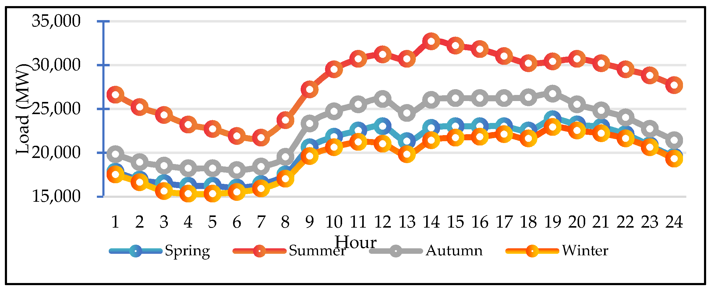
• Case 1: Based on the annual average daily load data of Taiwan’s power system.
• Case 2: Full-year simulation and testing of Taiwan’s power system.

For each case study, four specific tests are conducted:

• Test 1: An evaluation of optimal power flow in the power system.
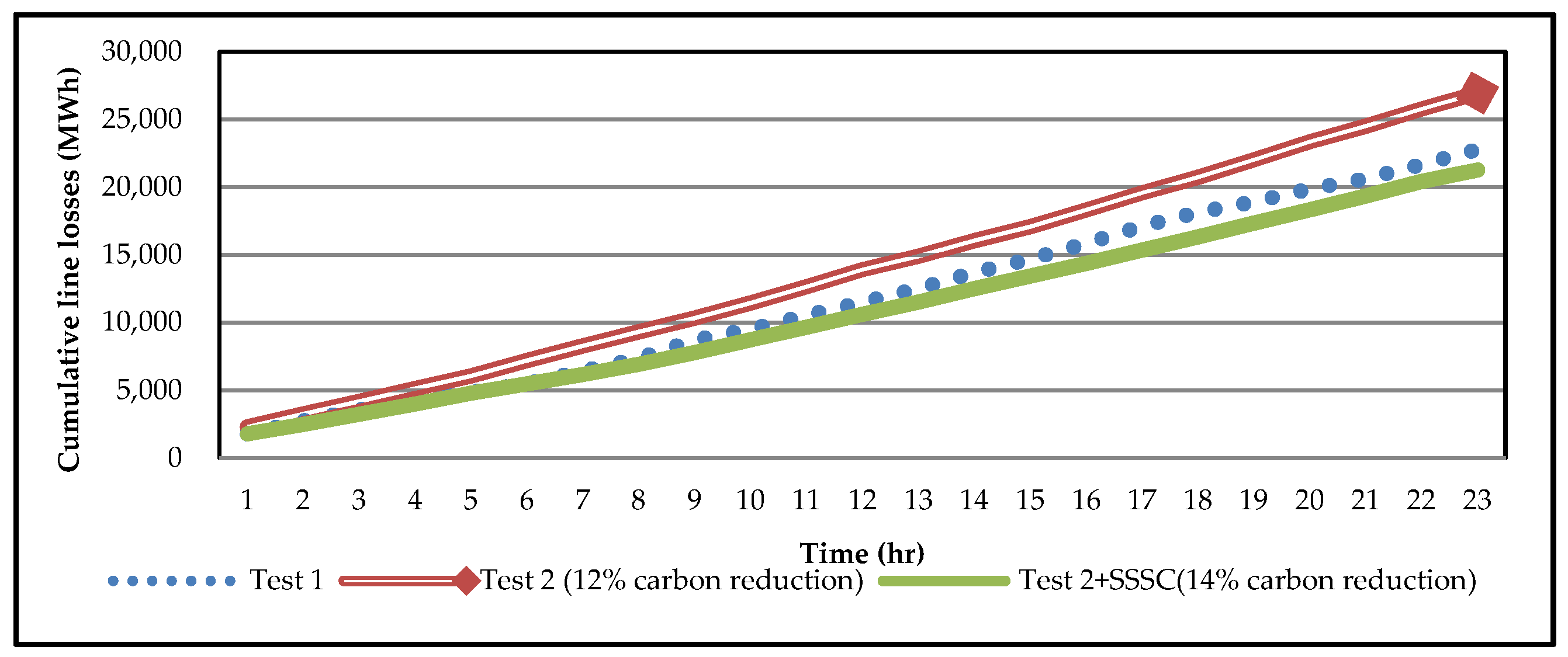
• Test 2: A profit-oriented carbon reduction analysis achieved through fuel-mix adjustments at the power company.
• Test 3: A detailed profit analysis of the power company’s participation in the carbon-trading market.
• Test 4: A profit analysis examining the joint participation of the power company and transmission operators (utilizing SSSC technology) in the carbon-trading market.

These tests aim to assess the efficiency of power flow optimization, evaluate carbon reduction strategies, and analyze the financial benefits of carbon trading under varying operational conditions.

The results should be discussed in relation to previous studies and the working hypotheses. The implications of the findings should be considered in the broadest possible context, and future research directions may also be highlighted.

5.1. Convergence Testing of the ATGA

This section performs an optimal power flow analysis for a single time period, validating the proposed ATGA’s feasibility by comparing it with GA [37], PSO [23], and PSO_TVAC [34]. All algorithms use 30 particles and run for 100 iterations. Under a total summer load demand of 32,707 MW, the ATGA demonstrates superior results, achieving higher profitability and lower carbon emissions. Specifically, as shown in

Table 1. Comparison of profit performance across algorithms.

Algorithm	Profit Min. (TWD)	Profit Avg. (TWD)	Profit Max. (TWD)	Execution Time (s)
GA	15,294,475	16,325,800	17,357,124	61.24
PSO	16,541,734	17,292,533	18,043,332	37.02
PSO_TVAC	17,333,620	18,453,572	19,573,524	32.71
ATGA	19,122,016	19,867,601	20,613,186	36.88

, ATGA outperforms the other algorithms with a maximum profit of TWD 20,613,186, while its average and minimum values are also higher than the others. Despite a slightly longer execution time, the significant increase in profit justifies its use.

As shown in

Table 2. Comparison of emissions performance across algorithms.

Algorithm	Emissions Min. (TWD)	Emissions Avg. (TWD)	Emissions Max. (TWD)	Execution Time (s)
GA	18,934.18	19,043.83	19,153.48	54.16
PSO	18,246.75	18,339.69	18,152.90	38.27
PSO_TVAC	18,049.78	18,152.90	18,256.02	33.74
ATGA	17,857.36	17,961.87	18,066.38	37.31

, the ATGA achieves a minimum carbon emission level of 17,857.36 tons, with average and maximum values consistently lower than GA, PSO, and PSO_TVAC, confirming its environmental efficiency.

The convergence results, illustrated in Figure 8 and Figure 9, demonstrate that ATGA converges faster and more reliably toward optimal profit and minimal carbon emissions. This superior convergence behavior, compared with other algorithms, underscores the algorithm’s efficiency and robustness in addressing dynamic economic dispatch problems.

Innovatively, this study integrates the equivalent current injection method, significantly improving the solution’s quality and reducing the execution time. This advancement makes the algorithm highly adaptable and reliable for complex power system optimization tasks. The integration of the hybrid gene concept with time-varying particle swarm optimization highlights the novelty of this approach, offering better performance while minimizing potential duplication risks in comparison with existing studies.

In this study, the proposed ATGA was used to determine the optimal installation location for the SSSC across different candidate lines. The objective was to maximize system profit by optimizing the placement of SSSC devices. Out of the 59 transmission lines in Taiwan’s power system, 7 lines were deemed unsuitable for SSSC installation, leaving 52 candidate lines for analysis, as shown in

Table 3. Candidate lines.

Candidate Lines No.	From	To
1	#9 Longtan	#10 Tatan
2	#14 Emei	#21 Zhongliao
3	#9 Longtan	#15 Tianlun
4	#25 Mailiao	#21 Zhongliao
5	#32 Renwu	#37 Gaogang
6	#27 Longqi	#30 Xingda
7	#42 Jiahui	#21 Zhongliao
8	#23 Fenglin	#40 Taitung
⋮	⋮	⋮
52	#29 Lubei	#31 Xingda

.

To perform the analysis, candidate locations for SSSC installation were selected based on the structural characteristics and power flow distribution of the network. The ATGA was then applied to each candidate line to evaluate the impact of SSSC installation. The optimization objective was to maximize system profit, and various combinations of candidate lines were tested to assess their performance under minimum, average, and maximum profit conditions.

Table 4. Profit performance comparison of candidate lines (Top 4).

Candidate Lines	Profit Min. (TWD)	Profit Avg. (TWD)	Profit Max. (TWD)
No. 1 + No. 2	208,433,240.5	222,543,792	236,654,344.0
No. 3 + No. 4	195,582,427.2	208,754,136	221,925,845.0
No. 5 + No. 6	156,682,469.5	182,977,425	209,272,380.3
No. 7 + No. 8	156,682,469.5	182,977,425	209,272,380.3

provides a comparison of the profit results across the different candidate line combinations.

The analysis shows that the combination of lines No. 1 + No. 2 yielded the highest profit, with a maximum value of TWD 236,654,344, significantly outperforming the other combinations. This indicates that installing SSSC on these specific lines can substantially enhance the system’s economic efficiency. On the other hand, the No. 5 + No. 6 combination produced the lowest minimum profit, at TWD 156,682,469.47, though it still presents a feasible option under certain conditions. Overall, the range of profits highlights the importance of selecting the optimal location for SSSC installation and further validates the efficiency and robustness of the ATGA in complex system optimization.

This data processing and result analysis demonstrates the effectiveness of SSSC installation across different candidate lines and successfully identifies the optimal placement combinations that maximize profit. The analysis provides valuable insights for the future deployment of SSSCs in power systems and showcases the practical and innovative contributions of the ATGA.

5.2. Case 1: Based on the Annual Average Daily Load Data

In continuation from the previous section, where the ATGA was successfully applied to solve the dynamic economic dispatch (DED) problem, the same approach was utilized to optimize both cost and carbon emissions in the following case studies. The four tests outlined in Section 5.1 provide a detailed exploration of how different strategies impact carbon reduction and profit maximization within Taiwan’s power system.

The optimization process generated by ATGA serves as the foundation for analyzing the various carbon reduction scenarios. The results from Tests 1 to 4, detailed in

Table 5. Annual daily average load test results.

Metrics	Test 1		Test 2 (Carbon Reduction 12%)		Test 3 (Carbon Reduction 30%)		Test 3 (Carbon Reduction 40%)		Test 3 (Carbon Reduction 50%)		Test 4 (Carbon Reduction 50%)
Total profit of power generators (TWD)	271,300,849		20,262,449		53,709,861		6,124,002		−28,027,552		−2,595,366
Total revenue of power generators (TWD)	1,774,734,960		1,774,734,960		1,774,734,960		1,774,734,960		1,774,734,960		1,774,734,960
Total expenditure of power generators (TWD)	1,503,434,111		1,754,472,511		1,720,961,032		1,768,546,891		1,802,762,512		1,777,330,326
Cost of Taipower generation (TWD)	828,419,472		1,035,019,927		1,035,019,927		1,035,019,927		1,035,019,927		1,004,719,118
Expenditure of power trading (TWD)	669,921,495		714,191,978		714,127,911		714,127,911		714,127,911		717,846,322
Carbon trading expenditure (TWD)					−33,447,412		14,138,447		48,354,068		42,130,030
Total profit of transmission operators (TWD)	5,093,144		5,260,606		5,260,606		5,260,606		5,260,606		12,634,856
Transmission fee (TWD)	5,093,144		5,260,606		5,260,606		5,260,606		5,260,606		5,272,011
Refund (TWD)											7,362,845
Total generation (MWh)	568,531.71		572,179.31		572,179.31		572,179.31		572,179.31		567,026.92
Taipower generation (MWh)	380,351.51		371,581.58		371,581.58		371,581.58		371,581.58		365,384.69
Power purchased from IPP (MWh)	188,180.2		200,597.73		200,597.73		200,597.73		200,597.73		201,642.23
Line losses (MWh)	22,786.71		26,959.03		26,959.03		26,959.03		26,959.03		21,281.92
Total pollution emissions (ton)	343,073.29		300,822.27		240,170.89		205,920.66		171,601.23		171,538.56
Total carbon emissions of all generators (ton)	343,073.29		300,822.27		300,822.27		300,822.27		300,822.27		294,527.7
Carbon trading volume (ton)			60,651.38		94,901.61		129,221.04		129,221.04		122,989.14
Coal (MWh)	144,426.59		57,862.95		57,862.95		57,862.95		57,862.95		55,092.26
Oil (MWh)	6781.75		13,174.15		13,174.15		13,174.15		13,174.15		10,724.63
Gas (MWh)	43,254.6		115,167.45		115,167.45		115,167.45		115,167.45		113,680.91

, offer insight into the effectiveness of both internal measures, such as fuel mix adjustments, and external mechanisms, like carbon trading and the use of advanced transmission technology (SSSCs), in reducing emissions and improving profitability. This study focuses on SSSCs as part of a market-based mechanism rather than comparing them with direct emissions-reduction technologies due to the distinct objectives and operational mechanisms of each approach. Since Taiwan currently lacks a carbon-trading market, the proposed SSSC and carbon trading integration aims to provide a scalable solution within the constraints of local policy frameworks.

Test 1 examines optimal power flow, while Test 2 evaluates profit-driven carbon reduction at Taipower. Tests 3 and 4 introduce carbon trading and SSSC integration, demonstrating how combining generation, transmission, and market strategies enhances sustainability and profitability.

Test 1: The first test primarily analyzed the OPF within Taiwan’s power system without any carbon reduction strategies. This baseline analysis established the operational efficiency and limitations of the existing grid infrastructure. The test results show that the total profit for power generators was TWD 271,300,849, with total revenue of TWD 1,774,734,960 and total expenditures of TWD 1,503,434,111. Since no external carbon-trading mechanisms were applied, this test serves as a reference for subsequent carbon-reduction strategies.

Test 2: In the second test, adjustments were made to Taipower’s fuel mix to maximize profit while achieving a 12% carbon reduction. The results showed a significant increase in generation costs, with total expenditure rising to TWD 1,754,472,511 and profit dropping to TWD 20,262,449. While carbon emissions were reduced by lowering coal usage and increasing gas-fired generation, this approach relied solely on internal optimizations, without the introduction of carbon trading. The diminishing returns in further emissions reductions were evident.

Test 3: The third test explored the effects of Taipower’s participation in the carbon-trading market, achieving 30%, 40%, and 50% carbon reduction targets. By purchasing carbon credits to offset emissions that could not be reduced through fuel adjustments alone, Taipower’s profit reached TWD 53,709,861 under the 30% reduction scenario. However, in the 40% and 50% reduction scenarios, the profit dropped significantly, to TWD 6,124,002 and a loss of TWD 2,595,366, respectively, reflecting the financial burden of increased carbon-trading costs.

Test 4: Taipower and transmission operators participated in the carbon-trading market while utilizing SSSC technology to further reduce transmission losses and carbon emissions. The implementation of SSSC technology reduced the need for power generators to purchase carbon credits, resulting in lower expenditures and an increased total profit of TWD 12,634,856. This test demonstrated that by enhancing transmission efficiency, the system achieved a 50% carbon reduction more effectively, reducing total emissions to 294,527.7 tons, and overall improving both economic performance and emissions reduction.

Additionally, this test introduced a feedback mechanism, where the power generators shared part of their carbon reduction benefits with the transmission operators. Specifically, based on reference [39], a 20% rebate was provided to transmission operators for their role in reducing emissions. As shown in Table 5, the total carbon emissions of all power generators in Test 3 (50% carbon reduction) and Test 4 (50% carbon reduction) were 300,822.27 tons and 294,527.70 tons, respectively. With the carbon price of TWD 5849/ton from Test 4 (50% carbon reduction), the rebate amount is calculated as shown in

Table 6. Detailed rebate calculation table.

Test Study	Total Carbon Emissions (ton)	Carbon Emission Difference (ton)	Carbon Price (TWD/ton)	Rebate Formula	Rebate Amount (TWD)
Test 3 (Carbon reduction 50%)	300,822.27	–	–	–	–
Test 4 (Carbon reduction 50%)	294,527.7	300,822.27–294,527.7	5849	5849 × (300,822.27 − 294,527.70) × 20%	7,362,845

. This novel approach of incentivizing transmission operators through shared benefits created a win-win scenario for both power generators and transmission operators. Not only did this strategy reduce carbon emissions more efficiently, but it also aligned the interests of both sectors in achieving environmental goals.

This study presents a unique framework by combining internal carbon reduction strategies with external market mechanisms, highlighting the role of SSSC technology in further enhancing system efficiency.

The comparative results of Tests 2, 3, and 4 show the progressive benefits of introducing carbon trading after maximizing internal fuel adjustments. While Test 2 achieved a 12% reduction in carbon emissions, deeper reductions, up to 50%, were made possible only with the integration of carbon-trading mechanisms in Test 3. This indicates that internal optimization alone is not sufficient to achieve aggressive carbon reduction targets, and carbon trading is a necessary component for balancing financial performance and environmental goals.

The role of SSSCs in enhancing carbon reduction in Test 4 highlights the significant role that SSSC technology plays in reducing transmission losses and carbon emissions. The SSSC’s ability to improve transmission efficiency directly impacted the overall carbon footprint of the system, allowing Taipower to achieve a 50% reduction in emissions with fewer carbon credits than in Test 3. This technological intervention demonstrates the importance of addressing transmission efficiency in addition to generation efficiency when targeting large-scale carbon reductions. Without carbon trading, Test 2 shows a 12% reduction in emissions by shifting from coal to oil- and gas-fired generation. Adding the SSSC further reduces emissions by 2% through minimizing transmission losses and optimizing fuel dispatch (Figure 10 and Figure 11).

The significant impact of incorporating SSSC technology highlights the potential for additional emissions reduction through enhanced transmission efficiency, even without participating in the carbon-trading market. Figure 12 illustrates the specific emissions reduction achieved, showing that on top of the fuel dispatch optimization, reducing line losses through the SSSC results in an additional 2% reduction in carbon emissions.

On the other hand, participation in the carbon-trading market becomes crucial. As depicted in Figure 13a, in Test 3, both power generators and transmission operators participated in carbon trading using a 24-h maximum profit strategy. In the carbon-trading market, the carbon purchase times were concentrated in the early morning hours (1:00–11:00), while carbon sales primarily occurred in the afternoon (12:00–18:00). This time distribution reflects the interaction between load fluctuations and carbon trading strategies within the power system.

Moreover, Figure 13b illustrates the comparison between the total profits of Test 3 and Test 4, both targeting a 50% carbon reduction. Despite the rebate mechanism introduced in Test 4, which requires power generators to share a portion of their profits with transmission operators (SSSC), the overall profit is still significantly higher than in Test 3. This indicates that despite the cost incurred by the rebate mechanism, the inclusion of SSSC technology leads to a noticeable improvement in both economic and environmental performance. Particularly, with the involvement of the carbon-trading market, a synergy between power generation and transmission is created, effectively reducing system losses and enhancing overall profitability.

The rebate mechanism in Test 4, where generators shared 20% of the carbon savings with transmission operators, fostered collaboration and improved transmission practices. Comparing Tests 3 and 4 shows that optimizing the network with SSSCs achieves carbon reductions more cost-effectively, minimizing financial losses and maximizing benefits. This study highlights that while internal measures offer modest reductions, significant progress relies on combining carbon trading and SSSC technology. Test 4 demonstrates how technological upgrades and financial incentives enable both generators and operators to benefit from reduced emissions.

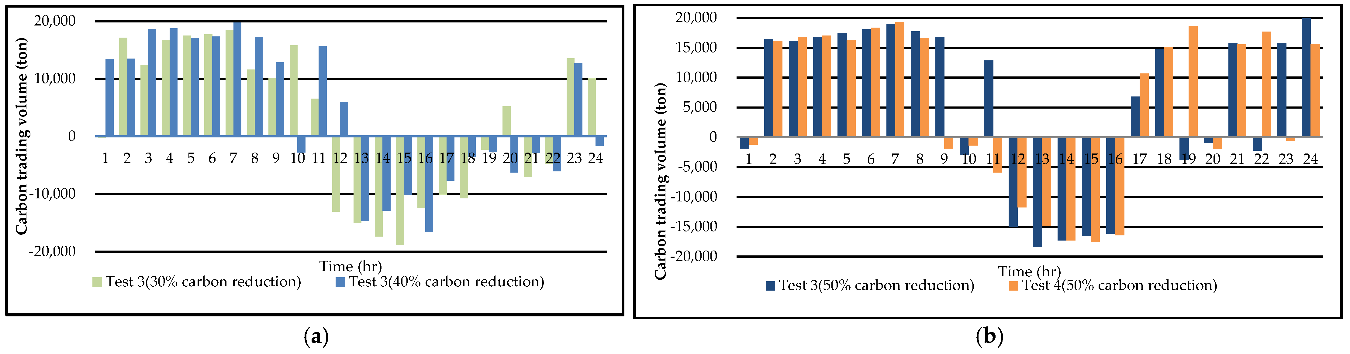
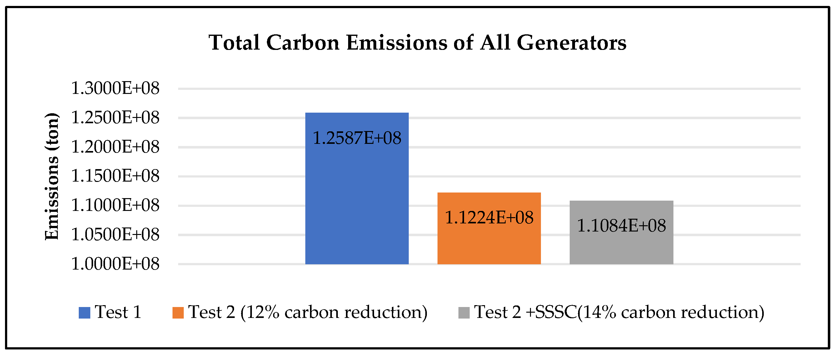
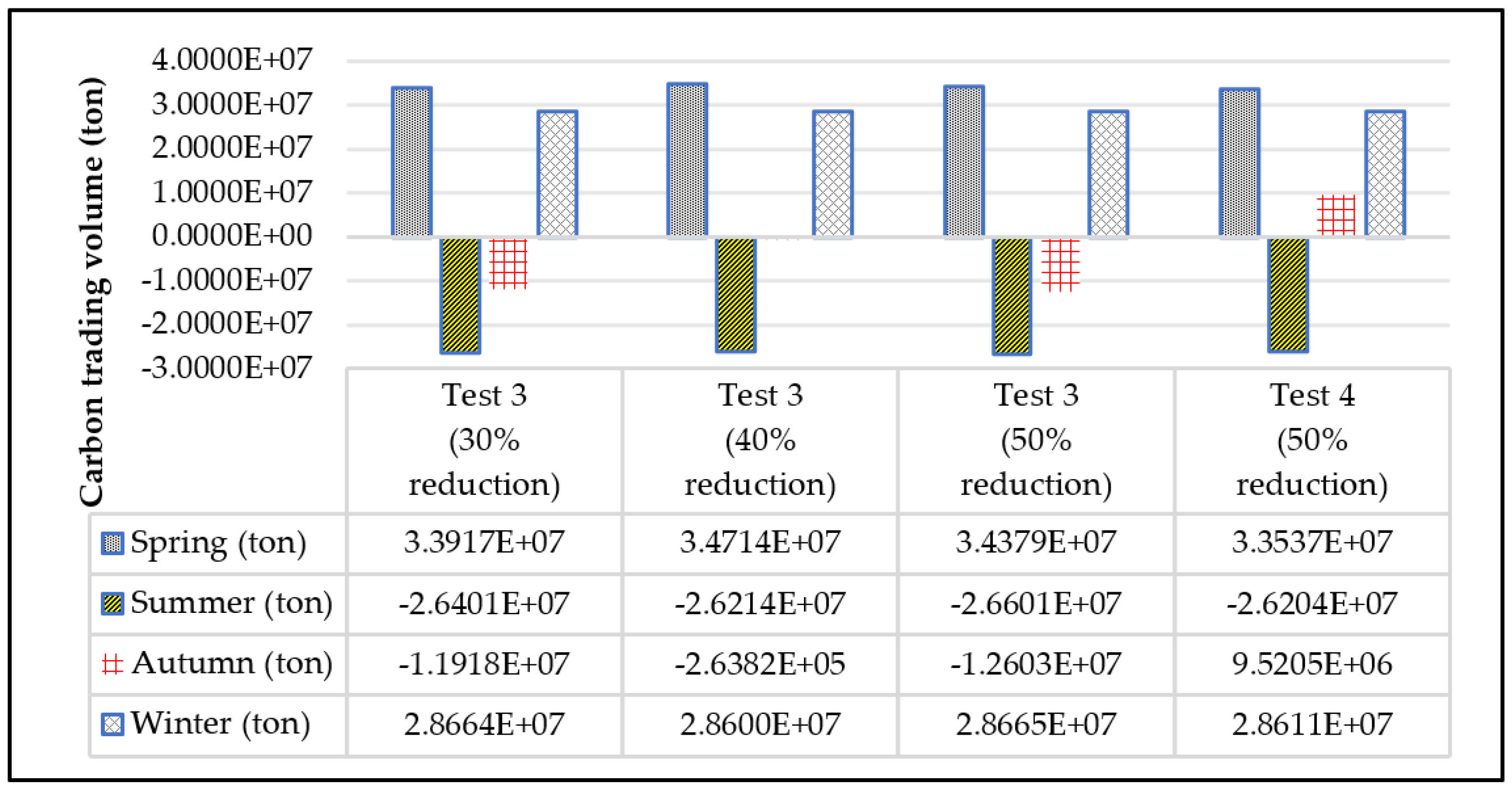
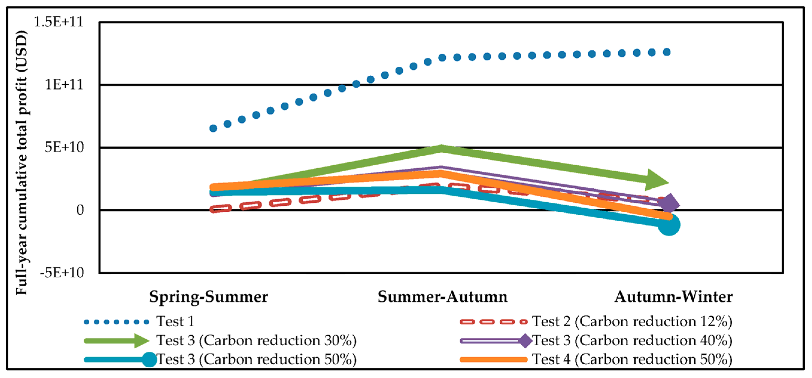
5.3. Case 2: Full-Year Simulation and Testing

Based on the data from Taiwan Power Company (Taipower), the system was simulated and tested using full-year load data to analyze the variations across different seasons and their impact on system performance. The seasonal load data are as follows [36]: 44,082,360 MW/h in spring, 60,657,120 MW/h in summer, 49,509,360 MW/h in autumn, and 42,219,360 MW/h in winter. These values demonstrate the fluctuations in electricity demand throughout the year, offering insights into the system’s operational performance under varying conditions. The data from Taipower ensures the accuracy and reliability of the simulation results.

This section analyzes

Table 7. Full-year average load test results.

Metrics	Test 1		Test 2 (Carbon Reduction 12%)		Test 3 (Carbon Reduction 30%)		Test 3 (Carbon Reduction 40%)		Test 3 (Carbon Reduction 50%)		Test 4 (Carbon Reduction 50%)
Total profit of power generators (109 TWD)	126.43		7.4913		21.798		5.0132		−11.396		−4.9236
Total revenue of power generators (1011 TWD)	6.3890		6.3890		6.3890		6.3890		6.3890		6.3890
Total expenditure of power generators (1011 TWD)	5.1247		6.3141		6.1711		6.3389		6.5030		6.4383
Cost of Taipower generation (1011 TWD)	2.8417		3.6701		3.6701		3.6701		3.6701		3.6056
Expenditure of power trading (1011 TWD)	2.2646		2.6252		2.6252		2.6252		2.6252		2.6235
Carbon trading expenditure (109 TWD)					2.4781		18.887		14.592		−14.306
Total profit of transmission operators (109 TWD)	1.8429		1.8804		1.8804		1.8804		1.8804		6.3301
Transmission fee (109 TWD)	1.8429		1.8804		1.8804		1.8804		1.8804		1.9111
Refund (109 TWD)											4.4190
Total generation (108 MWh)	2.0415		2.0609		2.0609		2.0609		2.0609		2.0366
Taipower generation (108 MWh)	1.4054		1.3235		1.3235		1.3235		1.3235		1.2997
Power purchased from IPP (107 MWh)	6.3613		7.3742		7.3742		7.3742		7.3742		7.3693
Line losses (106 MWh)	7.6810		9.6251		9.6251		9.6251		9.6251		7.1905
Total pollution emissions (107 ton)	12.587		11.239		8.8128		7.5552		6.3198		6.2934
Total carbon emissions of all generators (108 ton)	1.2587		1.1224		1.1224		1.1224		1.1224		1.0840
Carbon trading volume (107 ton)			2.4261		3.6837		4.9045		2.4261		4.5464
Coal (106 MWh)	56.401		12.385		12.385		12.385		12.385		9.4874
Oil (106 MWh)	2.2094		6.8665		6.8665		6.8665		6.8665		6.0631
Gas (106 MWh)	15.010		47.980		47.980		47.980		47.980		47.494

, focusing on Taiwan’s seasonal power operations and carbon reduction strategies. Without external mechanisms like carbon trading, internal adjustments achieve only an 11% emissions reduction, mainly by optimizing the generation mix (e.g., reducing coal and increasing natural gas). However, further reductions would risk profitability.

When the carbon-trading market is introduced, the potential for emissions reduction increases significantly. In the scenario targeting a 40% carbon reduction, the system leverages the carbon-trading market to offset emissions that cannot be reduced internally, while maintaining profitability. According to the data in Table 7, the total generation cost for Taipower remains consistent across the tests, at approximately TWD 6.31 × 10¹¹. Through effective participation in the carbon-trading market, Taipower can achieve substantial emissions reduction without incurring financial losses.

In Test 4, the SSSC technology is incorporated, and further emissions reductions are pursued through the carbon-trading market, achieving a 50% reduction in carbon emissions. When comparing Test 4 with Test 3 (both targeting 50% carbon reduction), Test 4 shows a significant reduction in financial losses. Specifically, Test 4’s power trading expenditure is TWD 6.3301 × 10⁹, compared with TWD 1.8804 × 10⁹ in Test 3. While Test 4 incurs higher power trading costs, it benefits from improved system efficiency, reducing transmission losses and minimizing the need for additional carbon credits.

Table 7 shows similar generation, line losses, and emissions reductions in Tests 3 and 4, both achieving a 50% reduction target. However, Test 4 achieves this more efficiently, with reduced financial losses through advanced technology. Integrating the carbon market and SSSCs enhances emissions reduction, lowers losses, and optimizes costs, ensuring both profitability and sustainability.

Installing SSSC technology reduces line losses and carbon emissions, enabling power generators to lower carbon credit purchases. Generators allocate part of their savings as rebates to transmission operators, proportional to the emissions reductions (

Table 8. Detailed rebate calculation table in case 2.

Test Study	Total Carbon Emissions (ton)	Carbon Emission Difference (ton)	Carbon Price (TWD/ton)	Rebate Formula	Rebate Amount (TWD)
Test 3 (carbon reduction 50%)	113,801,849.9	–	–	–	–
Test 4 (carbon reduction 50%)	109,903,518.5	113,801,849.9– 109,903,518.5	5667	5667 × (113,801,849.9 − 109,903,518.5) × 20%	4,117,992,957

). In Test 3, emissions totaled 113.8 million tons, while in Test 4, they dropped to 109.9 million tons, resulting in a rebate of approximately TWD 4.117 billion. This demonstrates how SSSC technology improves efficiency, reduces emissions, and provides economic incentives within the carbon-trading market.

Figure 14 shows that Taiwan Power Company, without participating in the carbon-trading market, can achieve a maximum carbon reduction of 11% through internal adjustments, as seen in Test 2. This is primarily due to fuel mix changes such as reducing coal usage. To further reduce emissions, incorporating SSSC technology enables an additional 3% reduction, bringing the total reduction to 14%. This improvement, demonstrated in Test 2 + SSSC, lowers emissions from 1.2587 × 10⁸ tons to 1.1084 × 10⁸ tons by optimizing transmission efficiency and reducing line losses. This highlights the limitation of autonomous carbon reduction, which reaches its peak at 14% without external market mechanisms.

Figure 15 illustrates the changes in power generation by fuel type under different carbon reduction scenarios. In Test 1, without any carbon reduction measures, coal generation is the highest, at 5.64 × 10⁷ MWh, followed by gas at 1.50 × 10⁷ MWh and oil at 2.21 × 10⁶ MWh. In Test 2, which achieves a 12% carbon reduction, coal generation significantly decreases to 1.24 × 10⁷ MWh, while gas increases substantially to 4.80 × 10⁷ MWh. Oil generation also rises to 6.87 × 10⁶ MWh. This shift reflects the strategy of reducing coal dependency and increasing cleaner fuel usage to lower emissions. Finally, in Test 2 + SSSC (14% carbon reduction), coal usage is further reduced to 9.49 × 10⁶ MWh, while gas remains stable at 4.75 × 10⁷ MWh. Oil usage slightly decreases to 6.06 × 10⁶ MWh. The introduction of the SSSC further optimizes fuel efficiency, reducing reliance on coal and oil while maintaining gas as a primary energy source, thereby achieving a higher level of carbon reduction.

In this case study, a full-year carbon emission test is conducted, as illustrated in Figure 16. Since carbon credits can be stored, the results show that under Test 3 (30% reduction), a significant number of carbon credits is sold during the summer and autumn, while in spring and winter, large numbers of credits are purchased. This seasonal trading strategy enables a 30% reduction in emissions. Specifically, in Test 3 (30% reduction), summer carbon sales reached −2.6401 × 10⁷ tons, while spring purchases were 3.3917 × 10⁷ tons. As the carbon reduction target increases to 40% in Test 3 (40% reduction), a notable shift occurs. During the summer, there is still a significant sale of carbon credits at −2.6214 × 10⁷ tons, but in the autumn, only a minimal amount is sold (−2.6382 × 10⁵ tons). This reduction in sales during the autumn reflects the limits imposed by the higher reduction target, making it more challenging to sell credits without risking non-compliance. In Test 4, aiming for a 50% reduction, the situation becomes even more stringent. With such a high reduction target, the system requires substantial carbon purchases during spring (3.3537 × 10⁷ tons) and winter (2.8611 × 10⁷ tons), while the summer continues to see heavy sales at −2.6204 × 10⁷ tons. The data show that achieving a 50% reduction necessitates large-scale carbon credit transactions across the seasons, especially in spring and winter, when significant purchases are needed to balance the system’s emissions.

Taiwan Power Company, when participating in the carbon-trading market with a 50% reduction goal, faces considerable financial strain due to the high cost of purchasing carbon credits. As a result, they may seek to offset this cost by purchasing reduced carbon quotas from transmission operators, which provides a more cost-effective solution while still ensuring compliance with the reduction targets. This approach allows for both substantial emissions reduction and minimized financial impact, as demonstrated by the data in Figure 16.

Figure 17 shows seasonal impacts on profitability tied to carbon reduction strategies. In Test 3 (50% reduction), profits drop sharply in autumn–winter, ending at TWD −2 × 10¹⁰, due to low demand. Test 4, with SSSC integration, stabilizes performance by reducing transmission losses, mitigating declines, and ensuring more balanced, sustainable outcomes across seasons.

6. Conclusions

This study successfully demonstrates the effectiveness of integrating the ATGA with SSSC technology within Taiwan’s power market. Through dynamic economic dispatch simulations and case studies, the following key findings are summarized:

(1)

Enhanced emissions reduction: Test 4 demonstrated a 50% reduction in carbon emissions, with total emissions reduced from 113.8 million tons (Test 3) to 109.9 million tons. This was achieved through the SSSC technology’s ability to reduce transmission losses and improve efficiency.

(2)

Improved economic performance: The integration of SSSC-enabled power generators to reduce carbon credit purchases resulted in a TWD 4.118 billion rebate for transmission operators. This collaborative mechanism minimized financial losses while supporting environmental goals.

(3)

Increased system profitability: Compared with Test 3, Test 4 showed improved profitability for both sectors. Transmission operator profits increased from TWD 5.26 million to TWD 12.63 million, illustrating the financial benefits of advanced transmission technologies.

(4)

Scalable and adaptable framework: The proposed model provides a replicable framework for other regions, offering a balance between economic and environmental objectives. By combining market-based carbon solutions with advanced optimization algorithms, it addresses the challenges in constrained power markets.

Future research may focus on exploring the scalability of this model in different regulatory contexts and integrating additional grid technologies to further enhance system resilience and sustainability.

References

1. International Energy Agency (IEA). Global Energy Review: CO2 Emissions in 2021; IEA: Paris, France, 2021. [Google Scholar]
2. International Renewable Energy Agency (IRENA). Renewables Readiness Assessment: 2021; IRENA: Abu Dhabi, United Arab Emirates, 2021. [Google Scholar]
3. European Commission. EU Emissions Trading System (EU ETS); European Commission: Brussels, Belgium, 2022. [Google Scholar]
4. Liu, Z.-F.; Li, L.-L.; Liu, Y.-W.; Liu, J.-Q.; Li, H.-Y.; Shen, Q. The role of FACTS devices in enhancing power system stability. Energy 2021, 235, 121407. [Google Scholar] [CrossRef]
5. Alajrash, B.H.; Salem, M.; Swadi, M.; Senjyu, T.; Kamarol, M.; Motahhir, S. A comprehensive review of FACTS devices in modern power systems: Addressing power quality, optimal placement, and stability with renewable energy penetration. Energy Rep. 2024, 11, 5350–5371. [Google Scholar] [CrossRef]
6. Bordignon, M.; Gamannossi degl’Innocenti, D. Third Time’s a Charm? Assessing the Impact of the Third Phase of the EU ETS on CO2 Emissions and Performance. Sustainability 2023, 15, 6394. [Google Scholar] [CrossRef]
7. Cao, C.; Han, W.; Liu, Y. Impact of carbon trading market on photovoltaic power generation under grid parity policy. In Proceedings of the 2022 Power System and Green Energy Conference (PSGEC), Shanghai, China, 25–27 August 2022. [Google Scholar]
8. Hawkes, A.D. Long-Run Marginal CO2 Emissions Factors in National Electricity Systems. Appl. Energy 2014, 125, 197–205. [Google Scholar] [CrossRef]
9. Kung, S.-S.; Li, H.; Kung, C.-C. Prospects of Taiwan’s solar energy development and policy formulation. Heliyon 2024, 10, e23811. [Google Scholar] [CrossRef] [PubMed]
10. Sen, S.; Ganguly, S. Opportunities, Barriers and Issues with Renewable Energy Development: A Discussion. Renew. Sustain. Energy Rev. 2017, 69, 1170–1181. [Google Scholar] [CrossRef]
11. Rashed, G.I.; Otuo-Acheampong, D.; Mensah, A.A.; Haider, H. Fault Analysis of Power System Transient Stability with Thyristor-Controlled Series Capacitor (TCSC). Electrica 2023, 23, 475–491. [Google Scholar] [CrossRef]
12. Wang, L.; Liu, X.; Li, Y.; Chang, D.; Ren, X. Low-Carbon Optimal Dispatch of Integrated Energy System Considering Demand Response under the Tiered Carbon Trading Mechanism. Electr. Power Constr. 2024, 45, 102–114. [Google Scholar]
13. Hu, C.; Cai, X.; Zhao, X.; Luo, S.; Lu, H.; Li, X. Carbon trading-based layered operation optimization of the electric–thermal multi-energy-flow coupling system with photothermal power stations. Front. Energy Res. 2023, 11, 1252414. [Google Scholar] [CrossRef]
14. Zhang, W.; Ji, C.; Liu, Y.; Hao, Y.; Song, Y.; Cao, Y.; Qi, H. Dynamic interactions of carbon trading, green certificate trading, and electricity markets: Insights from System Dynamics Modeling. PLoS ONE 2024, 19, e0304478. [Google Scholar] [CrossRef]
15. Hong, Q.; Cui, L.; Hong, P. The impact of carbon emissions trading on energy efficiency: Evidence from quasi-experiment in China’s carbon emissions trading pilot. Energy Econ. 2022, 110, 106025. [Google Scholar] [CrossRef]
16. Wang, L.; Zhao, H.; Wang, D.; Dong, F.; Feng, T.; Xiong, R. Low-Carbon Economic Dispatch of Integrated Energy System Considering Expanding Carbon Emission Flows. IEEE Access 2024, 12, 104755–104769. [Google Scholar] [CrossRef]
17. Li, J.; Xiang, Y.; Gu, C.; Sun, W.; Wei, X.; Cheng, S.; Liu, J. Formulation of Locational Marginal Electricity-Carbon Price in Power Systems. CSEE J. Power Energy Syst. 2023, 9, 1968–1972. [Google Scholar]
18. Liu, X.; Chen, W.; Han, D. Carbon pricing and its impact on power sector transition. Energy Rep. 2022, 8, 3341–3351. [Google Scholar]
19. Ellerman, A.D.; Buchner, B.K.; Carraro, C. The European Union Emissions Trading Scheme: Origins, allocation, and early results. Rev. Environ. Econ. Policy 2016, 10, 89–112. [Google Scholar] [CrossRef]
20. Deb, S.; Houssein, E.H.; Said, M. Performance of turbulent flow optimization on economic load dispatch. IEEE Access 2021, 9, 77882–77893. [Google Scholar] [CrossRef]
21. Yang, X.; Zhang, J.; Bi, L.; Jiang, Y. Does China’s Carbon Trading Pilot Policy Reduce Carbon Emissions? Empirical Analysis from 285 Cities. Int. J. Environ. Res. Public Health 2023, 20, 4421. [Google Scholar] [CrossRef]
22. Wang, G.; Ma, H.; Wang, B.; Alharbi, A.M.; Wang, H.; Ma, F. Multi-Objective Optimal Power Flow Calculation Considering Carbon Emission Intensity. Sustainability 2023, 15, 16953. [Google Scholar] [CrossRef]
23. Fang, J.; Li, Y.; Zou, H.; Ma, H.; Wang, H. Optimal Scheduling of Microgrids Considering Offshore Wind Power and Carbon Trading. Processes 2024, 12, 1278. [Google Scholar] [CrossRef]
24. Khan, T.A.; Ling, S.H. An Improved Gravitational Search Algorithm for Solving an Electromagnetic Design Problem. J. Comput. Electron. 2020, 19, 773–779. [Google Scholar] [CrossRef]
25. Liu, X.; Li, X.; Tian, J.; Yang, G.; Wu, H.; Ha, R.; Wang, P. Low-Carbon Economic Dispatch of Integrated Electricity-Gas Energy System Considering Carbon Capture, Utilization and Storage. IEEE Access 2023, 11, 25077–25089. [Google Scholar] [CrossRef]
26. Alghamdi, H.; Guanghua, L.; Riaz, M.; Hafeez, G.; Ullah, S. An Optimal Power Flow Solution for a Power System Integrated with Renewable Generation. AIMS Math. 2024, 9, 6603–6627. [Google Scholar] [CrossRef]
27. Nagarajan, K.; Rajagopalan, A.; Bajaj, M.; Sitharthan, R.; Mohammadi, S.A.D.; Blazek, V. Optimizing Dynamic Economic Dispatch through an Enhanced Cheetah-Inspired Algorithm for Integrated Renewable Energy and Demand-Side Management. Sci. Rep. 2024, 14, 3091. [Google Scholar] [CrossRef] [PubMed]
28. Zhang, M.; Wang, B.; Wei, J. The Robust Optimization of Low-Carbon Economic Dispatching for Regional Integrated Energy Systems Considering Wind and Solar Uncertainty. Electronics 2024, 13, 3480. [Google Scholar] [CrossRef]
29. Chou, K.-T.; Liou, H.-M. Carbon Tax in Taiwan: Path Dependence and the High-Carbon Regime. Energies 2023, 16, 513. [Google Scholar] [CrossRef]
30. Ma, X.; Pan, Y.; Zhang, M.; Ma, J.; Yang, W. Impact of Carbon Emission Trading and Renewable Energy Development Policy on the Sustainability of Electricity Market: A Stackelberg Game Analysis. Energy Econ. 2024, 129, 107199. [Google Scholar] [CrossRef]
31. Tu, C.-S.; Yang, C.-Y.; Tsai, M.-T. An Optimal Phase Arrangement of Distribution Transformers under Risk Assessment. Energies 2020, 13, 5852. [Google Scholar] [CrossRef]
32. Gbadeyan, O.J.; Muthivhi, J.; Linganiso, L.Z.; Deenadayalu, N. Decoupling Economic Growth from Carbon Emissions: A Transition toward Low-Carbon Energy Systems—A Critical Review. Clean Technol. 2024, 6, 1076–1113. [Google Scholar] [CrossRef]
33. Luo, S.; Li, Q.; Pu, Y.; Xiao, X.; Chen, W.; Liu, S.; Mao, X. A Carbon Trading Approach for Heat-Power-Hydrogen Integrated Energy Systems Based on a Vickrey Auction Strategy. J. Energy Storage 2023, 72, 108613. [Google Scholar] [CrossRef]
34. Chang, C.-C.; Chang, K.-C.; Lin, Y.-L. Policies for Reducing the Greenhouse Gas Emissions Generated by the Road Transportation Sector in Taiwan. Energy Policy 2024, 191, 114171. [Google Scholar] [CrossRef]
35. Sofia, D.; Giuliano, A.; Gioiella, F.; Barletta, D.; Poletto, M. Modeling of an air quality monitoring network with high space-time resolution. Comput. Aided Chem. Eng. 2018, 43, 193–198. [Google Scholar]
36. Taiwan Power Company. Available online: http://www.taipower.com.tw/ (accessed on 1 November 2024).
37. Ekinci, S.; Can, Ö.; Ayas, M.Ş.; Izci, D.; Salman, M.; Rashdan, M. Automatic Generation Control of a Hybrid PV-Reheat Thermal Power System Using RIME Algorithm. IEEE Access 2024, 12, 26919–26930. [Google Scholar] [CrossRef]
38. European Commission. Energy, Climate Change, Environment. Available online: https://commission.europa.eu/energy-climate-change-environment_en (accessed on 2 November 2024).
39. Sood, Y.R.; Padhy, N.P.; Gupta, H.O. Assessment for feasibility and pricing of wheeling transactions under deregulated environment of power industry. Int. J. Electr. Power Energy Syst. 2004, 26, 163–171. [Google Scholar] [CrossRef]
Figure 1. The feasible framework of Taiwan’s carbon emissions trading system.
Processes 12 02639 g001
Figure 2. A π-equivalent model of the transmission line.
Processes 12 02639 g002
Figure 3. The structure of the SSSC.
Processes 12 02639 g003
Figure 4. The equivalent single-line diagram of the SSSC.
Processes 12 02639 g004
Figure 5. The modified model of the SSSC equivalent circuit.
Processes 12 02639 g005
Figure 6. Single-line diagram of Taiwan’s power system 345 kV.
Processes 12 02639 g006
Figure 7. Single-line diagram of Taiwan’s power system, 345 kV.
Processes 12 02639 g007
Figure 8. Convergence of maximum profit for each algorithm.
Processes 12 02639 g008
Figure 9. Convergence of minimum carbon emissions for each algorithm.
Processes 12 02639 g009
Figure 10. Total carbon emissions of all generators without a carbon-trading market.
Processes 12 02639 g010
Figure 11. Taipower fuel mix without carbon market participation.
Processes 12 02639 g011
Figure 12. Cumulative line loss curve.
Processes 12 02639 g012
Figure 13. Carbon trading volume under reduction scenarios over 24 h: (a) Test 3 (30% and 40%), (b) Test 3 (50%), and Test 4 (50%).
Processes 12 02639 g013
Figure 14. Total carbon emissions of all generators without a carbon-trading market in case 2.
Processes 12 02639 g014
Figure 15. Taipower fuel mix without carbon market participation in case 2.
Processes 12 02639 g015
Figure 16. Full-year carbon trading volume.
Processes 12 02639 g016
Figure 17. Full-year cumulative total profit curve of the power generation industry.
Processes 12 02639 g017