

Toward Optimal Design of a Factory Air Conditioning System Based on Energy Consumption Prediction


Abstract
1. Introduction
1.1. Background
- High temperature and humidity requirements: C, .
- High requirements in cleanliness level.
- High air exchange rates and large fresh air supply.
- The balance in the pressure gradient.
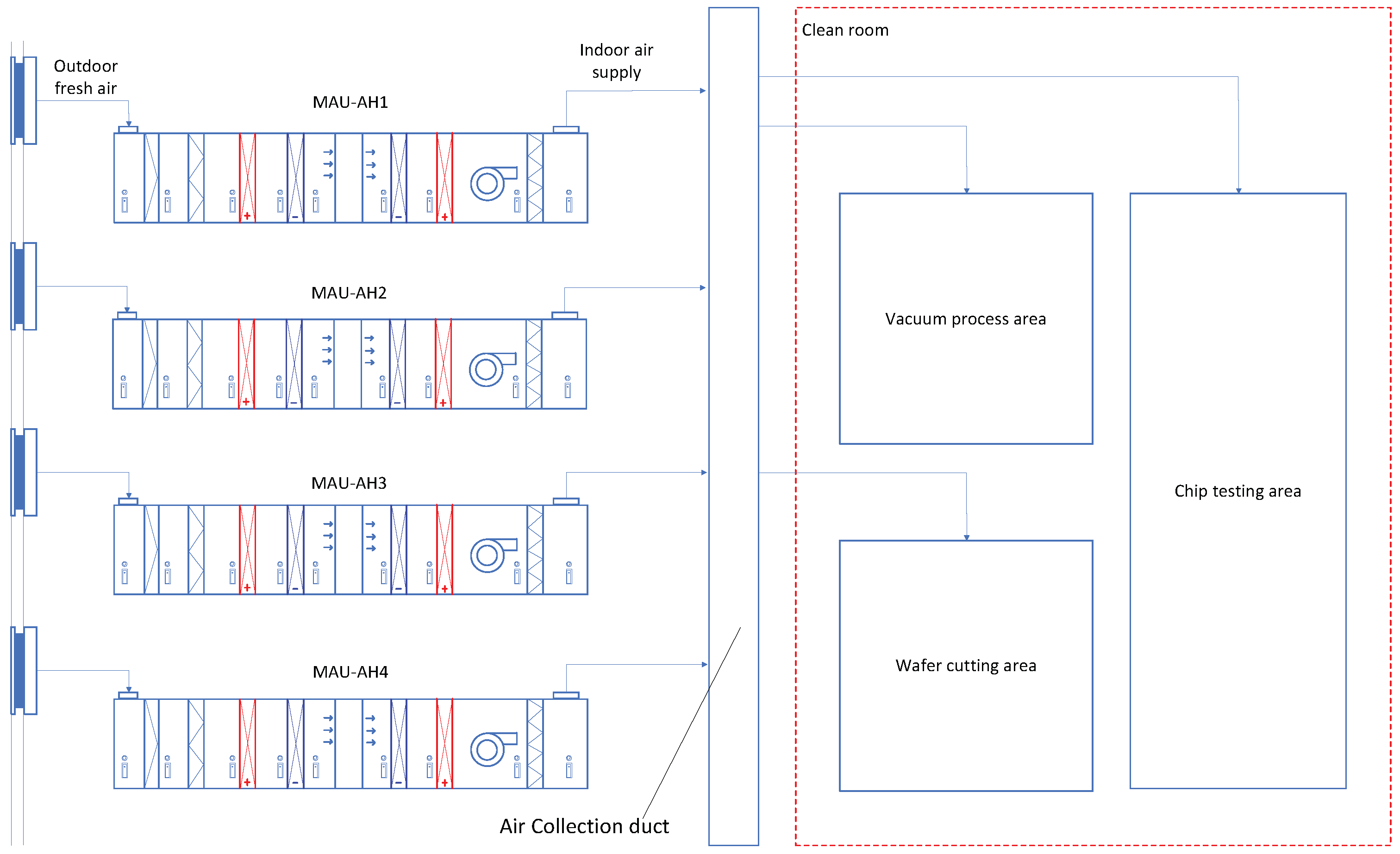
1.2. A Brief Introduction to the MAU’s Configuration and Control Strategy
2. Related Work and the Motivation
- The PID control parameters are manually set based on experience; however, the system (or the parameters of PID) without professional operators may result in energy wastage. For example, a common problem is excessive humidification by the humidifier of the MAU in winter mode, followed by dehumidification through the cooling coil.
- Following the above issue, the energy cost of the MAU has not been considered in the control criterion of traditional PID control. Moreover, the roles of the machine learning techniques in energy prediction have not been characterized well in the MAU system. Hence, there is significant room to optimize the energy consumption in the overall framework of the MAU, in addition to meeting the requirements of the supply air temperature and humidity.
- The effect of PID control could be poor when outdoor air conditions and supply air requirements are complex. Moreover, it cannot adaptively adjust the control parameters according to changes in indoor and outdoor environments and maintain an optimal control state at all times.
3. The Proposed MAU Energy-Saving Control Method
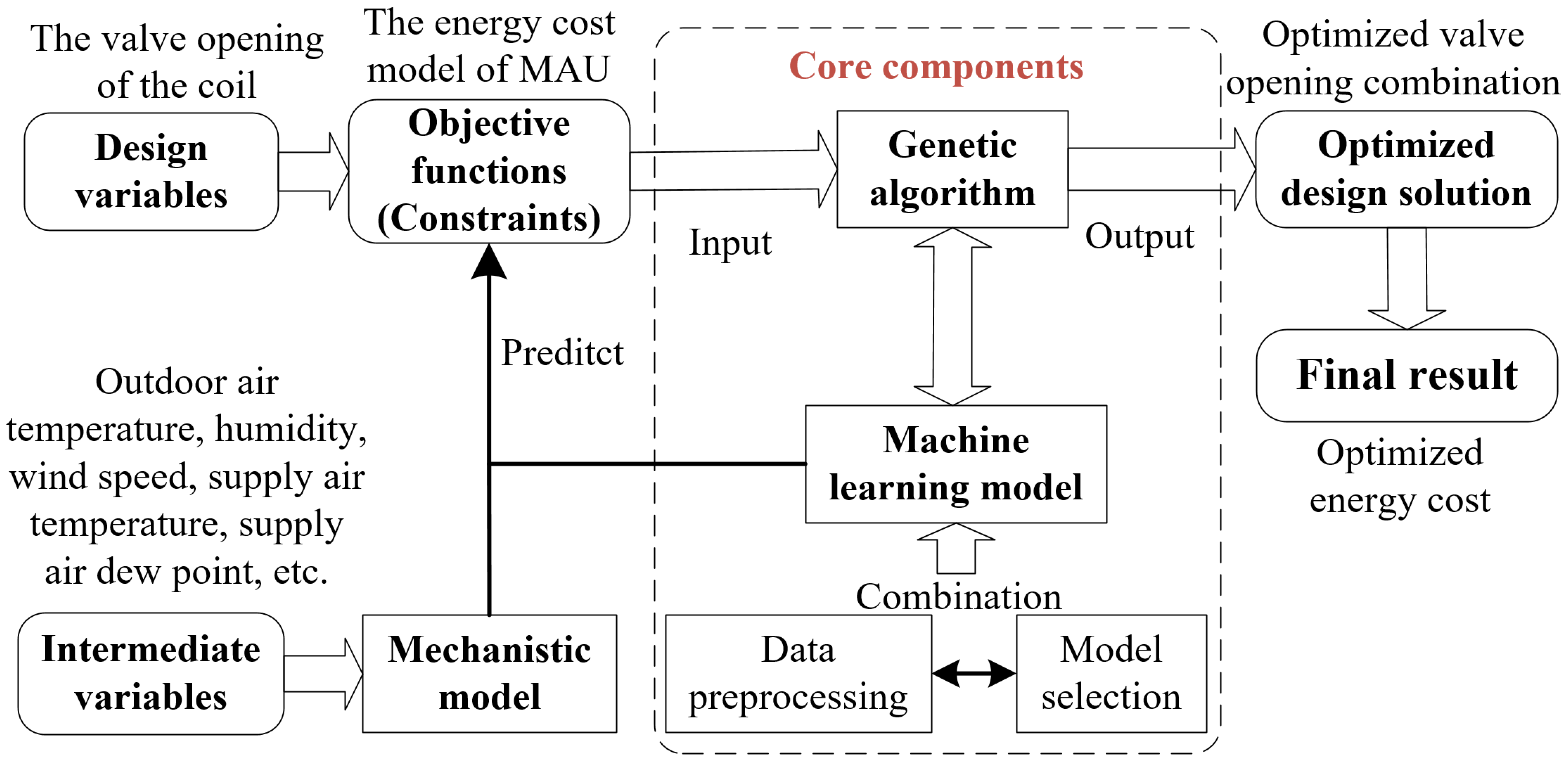
- Establish the energy consumption model of the MAU system: Based on the historical operation data of the MAU, we apply a machine learning algorithm to establish the data model. This model will correlate the coil opening with the energy supply of the MAU. Then, we can predict the temperature and the dew point of the supply air through an operation mechanism model of the MAU. Finally, the model is established to predict the MAU’s energy consumption for cold or hot water.
- Intelligent optimization method: It searches for the optimal coil opening to minimize energy consumption and achieve active energy-saving optimization.
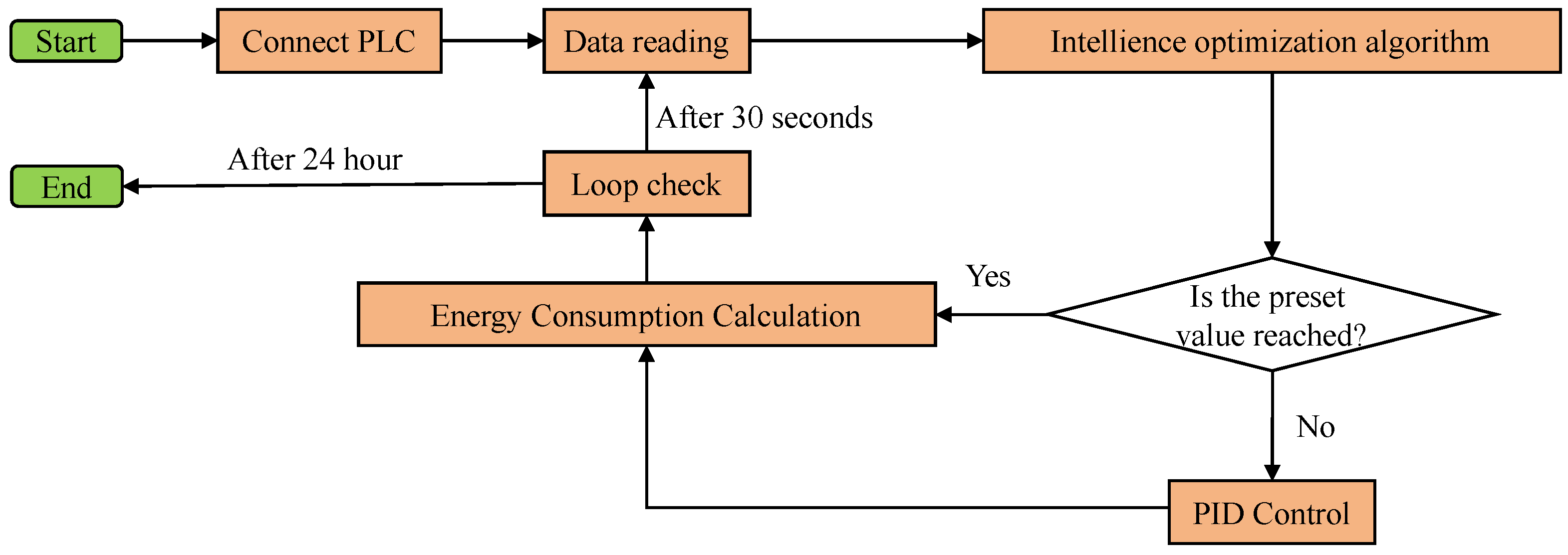
- Control the MAU according to the optimization results: The algorithm controls the MAU according to the optimized coil opening. It also calculates the deviation between the actual value and the set value and corrects the deviation with the PID algorithm.
- Monitor the outdoor air temperature and humidity conditions in real time: When the temperature or humidity changes, the algorithm re-optimizes the energy saving.
3.1. Mathematical Model of MAU
- Cooling only: The cooling treatment provided by the precooling coil only reduces the air temperature. Given the cooling capacity of the precooling coil denoted as , the energy conversion process in the precooling section can be expressed as follows:The air-specific enthalpy can be solved based on the above equation.
- Cooling with dehumidifying: The precooling coil performs both cooling and dehumidification treatment, which simultaneously reduces the air temperature and decreases the moisture content of the air. During this process, condensate water is produced, and given the cooling capacity of the precooling coil, denoted as , the energy conversion process in the precooling section can be expressed as follows:
3.2. The Data-Driven Model Based on Machine Learning Methods
3.2.1. Data Analysis
3.2.2. Data Pre-Processing
3.3. Machine Learning Algorithms
3.3.1. Linear Regression
3.3.2. Ridge Regression
3.3.3. Lasso Regression
3.3.4. K-Nearest Neighbors Regression
3.3.5. Decision Tree Regression
3.3.6. Random Forest Regression
3.3.7. Gradient Boosting Regression
3.3.8. AdaBoost Regression
3.4. Model Configuration and Performance Evaluation
3.5. Definition of the Optimization Problem
3.6. Direction-Based Optimization Algorithm
| Algorithm 1 Direction-based optimization algorithm |
|
3.6.1. Directional Crossover Operator
3.6.2. Directed Mutation Operator
4. Simulink Simulation Design
4.1. Simulation Model
4.2. Verification of the Model’s Reliability
5. Experiment
5.1. Data Visualization
- Preheating: In the preheating section, out of 25,000 historical datasets, 563 did not achieve an accuracy of 90% or higher in predictions, constituting approximately 2.1% of the total data sample. The prediction accuracy in the preheating section is illustrated in Figure 9a, while the specific comparison between the predicted values and true values for both the overall prediction accuracy and the instances wherein the standard was not met is illustrated in Figure 9b.
- Precooling: In the precooling section, out of 25,000 historical datasets, 965 did not achieve an accuracy of 90% or higher in predictions, constituting approximately 3.6% of the total data sample. The specific comparison between the predicted values and true values for both the overall prediction accuracy and the instances wherein the standard was not met is illustrated in Figure 10.
- Recooling: In the recooling section, out of 25,000 historical datasets, 352 did not achieve an accuracy of 90% or higher in predictions, constituting approximately 1.3% of the total data sample. The specific comparison between the predicted values and true values for the overall prediction accuracy and the instances wherein the standard was not met is illustrated in Figure 11.
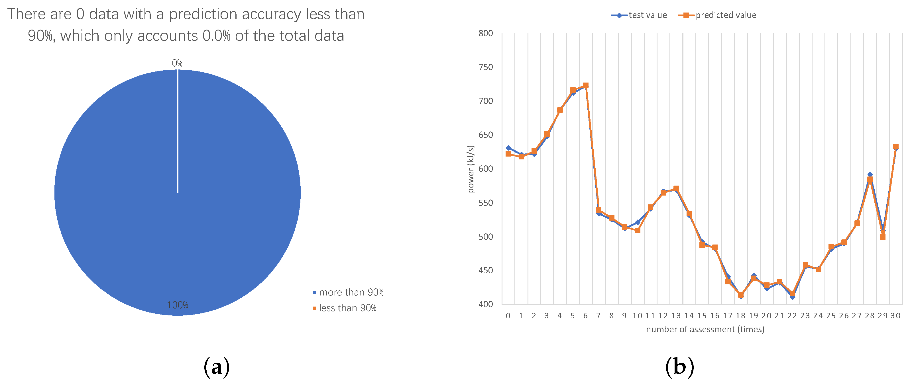
- Reheating: In the reheating stage, all 25,000 historical datasets achieved an accuracy of 90% or higher in predictions. The specific comparison between the predicted values and true values for the overall prediction accuracy and the instances wherein the standard was not met is illustrated in Figure 12.
5.2. Real Installation Design
5.3. The Experiment of Optimization Process
5.4. Simulation Experiment
- Experiment method:
- (a)
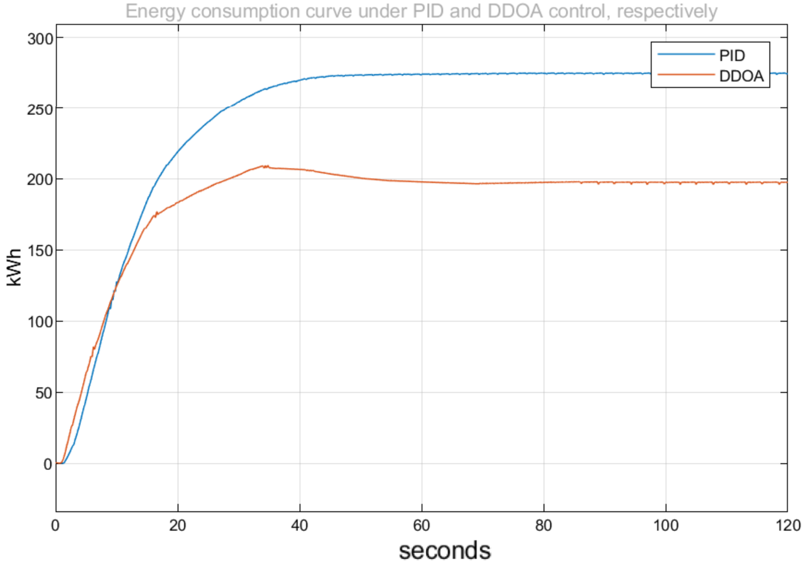
- Traditional PID control:
- Select several representative data from the dataset for the experiment.
- Run the simulation system based on the selected data using the traditional PID control method. This allows us to observe the energy consumption of the PID control method.
- (b)
- Intelligent optimization control:
- Run the proposed algorithm based on the selected data to obtain the setpoint for the pre-processing stage.
- Run the simulation system based on the selected data and the setpoint obtained from the pre-processing stage. Then, we can observe the energy consumption of the intelligent control method.
- Experiment result:
- (a)
- Experiment data:
- (b)
- Experimental configuration for traditional PID control:
- Preprocessing stage setpoint: C;
- Supply air dew point: C;
- Supply air temperature: C.
- (c)
- Experimental configuration for intelligent optimization control:
- Preprocessing stage setpoint: C;
- Supply air dew point: C;
- Supply air temperature: C.
- (d)
- Comparison of experimental results:
5.5. Detailed Analysis and Discussion of Experimental Results
6. Conclusions
Author Contributions
Funding
Data Availability Statement
Conflicts of Interest
References
- Zhuang, C.; Shan, K.; Wang, S. Coordinated demand-controlled ventilation strategy for energy-efficient operation in multi-zone cleanroom air-conditioning systems. Build. Environ. 2021, 191, 107588. [Google Scholar] [CrossRef]
- Zhao, W.; Li, H.; Wang, S. Energy performance and energy conservation technologies for high-tech cleanrooms: State of the art and future perspectives. Renew. Sustain. Energy Rev. 2023, 183, 113532. [Google Scholar] [CrossRef]
- Zhang, X.; Zhou, Y. Waste-to-energy (W2E) for renewable-battery-FCEV-building multi-energy systems with combined thermal/power, absorption chiller and demand-side flexibility in subtropical climates. Energy Build. 2024, 307, 113949. [Google Scholar] [CrossRef]
- Grassi, B.; Piana, E.A.; Lezzi, A.M.; Pilotelli, M. A review of recent literature on systems and methods for the control of thermal comfort in buildings. Appl. Sci. 2022, 12, 5473. [Google Scholar] [CrossRef]
- Li, L.; Gao, Y.; Ning, D.Z.; Yuan, Z.M. Development of a constraint non-causal wave energy control algorithm based on artificial intelligence. Renew. Sustain. Energy Rev. 2021, 138, 110519. [Google Scholar] [CrossRef]
- Prince; Hati, A.S. A comprehensive review of energy-efficiency of ventilation system using Artificial Intelligence. Renew. Sustain. Energy Rev. 2021, 146, 111153. [Google Scholar] [CrossRef]
- Sayed, E.T.; Olabi, A.G.; Elsaid, K.; Al Radi, M.; Semeraro, C.; Doranehgard, M.H.; Eltayeb, M.E.; Abdelkareem, M.A. Application of artificial intelligence techniques for modeling, optimizing, and controlling desalination systems powered by renewable energy resources. J. Clean. Prod. 2023, 413, 137486. [Google Scholar] [CrossRef]
- Wang, X.; Liu, S.; Xiong, L.; Wu, D.; Zhang, Y. Research on intelligent regulation of air conditioning energy saving based on human thermal comfort. J. Ambient. Intell. Humaniz. Comput. 2021, 1–14. [Google Scholar] [CrossRef]
- Bao, L.; Li, N.; Qin, H. Research on Energy-Saving Optimization of Variable Flow Air Conditioning Chilled Water System. In Future Energy: Challenge, Opportunity, and, Sustainability; Springer: Berlin/Heidelberg, Germany, 2023; pp. 187–198. [Google Scholar]
- Peng, Q.; Yang, G.; Du, Q. Energy-saving Optimization of Frequency-variable Heat Pump Air Conditioning System for Electric Vehicles Based on a Genetic Algorithm. Int. J. Automot. Technol. 2023, 24, 1543–1551. [Google Scholar] [CrossRef]
- Sun, T.; Huang, X.; Liang, C.; Liu, R.; Yan, Y. Energy Consumption and Energy Saving Analysis of Air-Conditioning Systems of Data Centers in Typical Cities in China. Sustainability 2023, 15, 7826. [Google Scholar] [CrossRef]
- Zhou, Y.; Dan, Z.; Yu, X. Climate-adaptive resilience in district buildings and cross-regional energy sharing in Guangzhou-Shenzhen-Hong Kong Greater Bay Area. Energy Build. 2024, 308, 114004. [Google Scholar] [CrossRef]
- Zhu, S.; Sun, N.; Lv, S.; Chen, K.; Fang, W.; Cao, L. Research progress on intelligent optimization techniques for energy-efficient design of ship hull forms. J. Membr. Comput. 2024, 1–17. [Google Scholar] [CrossRef]
- Fattahi, M.; Sharbatdar, M. Machine-learning-based personal thermal comfort modeling for heat recovery using environmental parameters. Sustain. Energy Technol. Assessments 2023, 57, 103294. [Google Scholar] [CrossRef]
- Zhou, Y.; Zheng, S.; Hensen, J.L. Machine learning-based digital district heating/cooling with renewable integrations and advanced low-carbon transition. Renew. Sustain. Energy Rev. 2024, 199, 114466. [Google Scholar] [CrossRef]
- Cui, M.; Li, L.; Zhou, M.; Abusorrah, A. Surrogate-assisted autoencoder-embedded evolutionary optimization algorithm to solve high-dimensional expensive problems. IEEE Trans. Evol. Comput. 2022, 26, 676–689. [Google Scholar] [CrossRef]
- Zhou, M.; Cui, M.; Xu, D.; Zhu, S.; Zhao, Z.; Abusorrah, A. Evolutionary optimization methods for high-dimensional expensive problems: A survey. IEEE/CAA J. Autom. Sin. 2024, 11, 1092–1105. [Google Scholar] [CrossRef]
- Sun, N.; Zhu, S. Modeling and Optimization of Energy Consumption in Data-driven Factory Air Conditioning System. In Proceedings of the Genetic and Evolutionary Computation Conference Companion, Melbourne, VIC, Australia, 14–18 July 2024; pp. 107–108. [Google Scholar]
- Zhu, S.; Xu, L.; Goodman, E.D. Hierarchical Topology-Based Cluster Representation for Scalable Evolutionary Multiobjective Clustering. IEEE Trans. Cybern. 2022, 52, 9846–9860. [Google Scholar] [CrossRef]
- Zhu, S.; Xu, L.; Goodman, E.D.; Lu, Z. A New Many-Objective Evolutionary Algorithm Based on Generalized Pareto Dominance. IEEE Trans. Cybern. 2022, 52, 7776–7790. [Google Scholar] [CrossRef]
- Maskooki, A.; Deb, K.; Kallio, M. A customized genetic algorithm for bi-objective routing in a dynamic network. Eur. J. Oper. Res. 2022, 297, 615–629. [Google Scholar] [CrossRef]
- Zhao, Z.; Zhou, M.; Liu, S. Iterated greedy algorithms for flow-shop scheduling problems: A tutorial. IEEE Trans. Autom. Sci. Eng. 2022, 19, 1941–1959. [Google Scholar] [CrossRef]
- Tan, Y.; Lian, L. Engineering Thermodynamics; Chemical Industry Press: Beijing, China, 2010. [Google Scholar]
- Kamiran, F.; Calders, T. Data preprocessing techniques for classification without discrimination. Knowl. Inf. Syst. 2011, 33, 1–33. [Google Scholar] [CrossRef]
- Noi, P.T.; Kappas, M. Comparison of Random Forest, k-Nearest Neighbor, and Support Vector Machine Classifiers for Land Cover Classification Using Sentinel-2 Imagery. Sensors 2017, 18, 18. [Google Scholar] [CrossRef] [PubMed]
- Gray, J.B. Introduction to Linear Regression Analysis. Technometrics 2002, 44, 191–192. [Google Scholar] [CrossRef]
- Hoerl, A.E.; Kennard, R.W. Ridge Regression: Biased Estimation for Nonorthogonal Problems. Technometrics 2000, 42, 80–86. [Google Scholar] [CrossRef]
- Lee, J.H.; Shi, Z.; Gao, Z. On LASSO for predictive regression. J. Econom. 2022, 229, 322–349. [Google Scholar] [CrossRef]
- Beskopylny, A.N.; Stel’makh, S.A.; Shcherban’, E.M.; Mailyan, L.R.; Meskhi, B.; Razveeva, I.; Chernil’nik, A.; Beskopylny, N. Concrete strength prediction using machine learning methods CatBoost, k-nearest neighbors, support vector regression. Appl. Sci. 2022, 12, 10864. [Google Scholar] [CrossRef]
- Charbuty, B.; Abdulazeez, A.M. Classification Based on Decision Tree Algorithm for Machine Learning. J. Appl. Sci. Technol. Trends 2021, 2, 20–28. [Google Scholar] [CrossRef]
- Belgiu, M.; Drăguţ, L.D. Random forest in remote sensing: A review of applications and future directions. Isprs J. Photogramm. Remote. Sens. 2016, 114, 24–31. [Google Scholar] [CrossRef]
- Chen, T.; Guestrin, C. XGBoost: A Scalable Tree Boosting System. In Proceedings of the 22nd ACM SIGKDD International Conference on Knowledge Discovery and Data Mining, San Francisco, CA, USA, 13–17 August 2016; pp. 785–794. [Google Scholar] [CrossRef]
- Ke, G.; Meng, Q.; Finley, T.; Wang, T.; Chen, W.; Ma, W.; Ye, Q.; Liu, T.Y. Lightgbm: A highly efficient gradient boosting decision tree. In Proceedings of the 31st International Conference on Neural Information Processing Systems (NIPS’17), Long Beach, CA, USA, 4–9 December 2017; Curran Associates Inc.: Red Hook, NY, USA, 2017; pp. 3149–3157. [Google Scholar]
- Hastie, T.J.; Rosset, S.; Zhu, J.; Zou, H. Multi-class AdaBoost. Stat. Its Interface 2009, 2, 349–360. [Google Scholar] [CrossRef]
- Smola, A.; Scholkopf, B. A tutorial on support vector regression. Stat. Comput. 2004, 14, 199–222. [Google Scholar] [CrossRef]
- Deb, K.; Pratap, A.; Agarwal, S.; Meyarivan, T. A fast and elitist multiobjective genetic algorithm: NSGA-II. IEEE Trans. Evol. Comput. 2002, 6, 182–197. [Google Scholar] [CrossRef]
- Cheng, R.; Jin, Y.; Olhofer, M.; sendhoff, B. Test Problems for Large-Scale Multiobjective and Many-Objective Optimization. IEEE Trans. Cybern. 2017, 47, 4108–4121. [Google Scholar] [CrossRef] [PubMed]
- Ghosh, A.; Deb, K.; Goodman, E.; Averill, R. A user-guided innovization-based evolutionary algorithm framework for practical multi-objective optimization problems. Eng. Optim. 2023, 55, 2084–2096. [Google Scholar] [CrossRef]
- Zhang, Q.; Li, H. MOEA/D: A Multiobjective Evolutionary Algorithm Based on Decomposition. IEEE Trans. Evol. Comput. 2007, 11, 712–731. [Google Scholar] [CrossRef]
- Blank, J.; Deb, K. Pymoo: Multi-objective optimization in python. IEEE Access 2020, 8, 89497–89509. [Google Scholar] [CrossRef]
- Price, K.V. Differential Evolution. In Handbook of Optimization: From Classical to Modern Approach; Springer: Berlin/Heidelberg, Germany, 2013; pp. 187–214. [Google Scholar] [CrossRef]
- Cai, Z.; Gao, S.; Yang, X.; Zhou, M. Multiselection-Based Differential Evolution. IEEE Trans. Syst. Man, Cybern. Syst. 2024. [Google Scholar] [CrossRef]
- Sun, J.; Fang, W.; Wu, X.; Palade, V.; Xu, W. Quantum-behaved particle swarm optimization: Analysis of individual particle behavior and parameter selection. Evol. Comput. 2012, 20, 349–393. [Google Scholar] [CrossRef]
- Li, X.; Fang, W.; Zhu, S. An improved binary quantum-behaved particle swarm optimization algorithm for knapsack problems. Inf. Sci. 2023, 648, 119529. [Google Scholar] [CrossRef]
- Meshram, P.M.; Kanojiya, R.G. Tuning of PID controller using Ziegler-Nichols method for speed control of DC motor. In Proceedings of the IEEE-International Conference On Advances In Engineering, Science And Management (ICAESM-2012), Nagapattinam, India, 30–31 March 2012; pp. 117–122. [Google Scholar]
- Borase, R.P.; Maghade, D.K.; Sondkar, S.Y.; Pawar, S.N. A review of PID control, tuning methods and applications. Int. J. Dyn. Control. 2021, 9, 818–827. [Google Scholar] [CrossRef]
- Lyu, W.; Li, X.; Shi, W.; Wang, B.; Huang, X. A general method to evaluate the applicability of natural energy for building cooling and heating: Revised degree hours. Energy Build. 2021, 250, 111277. [Google Scholar] [CrossRef]
- Hassan, M.A.; Abdelaziz, O. Best practices and recent advances in hydronic radiant cooling systems–Part II: Simulation, control, and integration. Energy Build. 2020, 224, 110263. [Google Scholar] [CrossRef]


| Symbol | Meaning |
|---|---|
| h | Air-specific enthalpy |
| Q | The actual amount of cooling or heating provided by the coil to the air per unit time |
| m | Air mass flow rate |
| T | Air temperature |
| d | Air moisture content, kg water/kg dry air |
| , , , , , | |
| Heat transfer efficiency | |
| c | The specific heat capacity of water |
| The density of water | |
| f(TCV) | The flow characteristic of the coil control valve |
| Model | RMSE | R Squared |
|---|---|---|
| Linear Regression | 15.892662 | 0.995577 |
| Ridge Regression | 15.892681 | 0.995577 |
| Lasso Regression | 15.928640 | 0.995557 |
| K Neighbors Regressor | 12.711077 | 0.997171 |
| Decision Tree Regressor | 13.526912 | 0.996800 |
| Random Forest Regressor | 11.162434 | 0.997822 |
| Gradient Boosting Regressor | 13.578922 | 0.996771 |
| Adaboost Regressor | 25.567316 | 0.988897 |
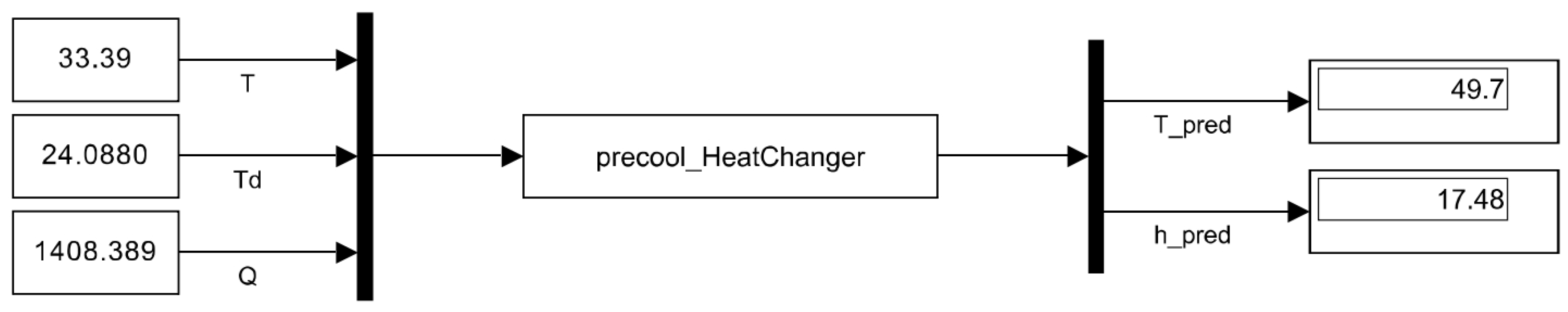
| Air Temperature (°C) | Air Dew Point (°C) | Q (kJ/s) | Temperature After Cooling (°C) | Specific Enthalpy After Cooling (kJ/kg) |
|---|---|---|---|---|
| 33.39 | 24.0880 | 1408.389 | 49.7023 | 17.48 |
| T_env | d_env | T_SP | Td_SP | kWh | |||
|---|---|---|---|---|---|---|---|
| AESOC-GA | AESOC-DE | AESOC-PSO | PID | ||||
| 32.25 | 16.01 | 19.97 | 9.18 | 152.45 (25.19) | 244.20 (6.713) | 156.63 (19.26) | 226.30 |
| 27.55 | 19.41 | 19.96 | 10.16 | 143.51 (2.42) | 168.03 (24.10) | 198.80 (13.80) | 162.53 |
| 31.65 | 19.12 | 20.12 | 9.36 | 223.20 (0.82) | 222.02 (0.02) | 213.88 (49.91) | 228.23 |
| 23.06 | 10.80 | 21.06 | 11.11 | 17.07(7.06) | 15.66 (7.27) | 20.94 (18.79) | 76.15 |
| 22.85 | 15.45 | 18.88 | 10.19 | 51.42 (54.68) | 73.87 (25.89) | 72.128 (6.95) | 108.13 |
| 24.41 | 17.82 | 19.15 | 12.02 | 43.24 (36.31) | 61.04 (32.70) | 127.51 (57.28) | 54.50 |
| 23.66 | 10.52 | 21.20 | 10.86 | 13.15(3.23) | 9.06 (1.68) | 5.00 (9.88) | 77.28 |
| 26.87 | 14.55 | 18.81 | 9.65 | 107.55 (2.42) | 106.49 (12.12) | 110.2 (12.89) | 96.01 |
| 34.68 | 21.36 | 20.19 | 8.97 | 137.35 (169.08) | 310.75 (103.84) | 268.75 (96.47) | 224.86 |
| 29.63 | 13.10 | 20.84 | 10.27 | 72.40 (3.06) | 66.64 (4.86) | 88.42 (26.67) | 237.67 |
| 25.91 | 15.98 | 21.13 | 10.57 | 85.53 (20.72) | 73.65 (31.73) | 55.76 (51.66) | 241.46 |
| 26.10 | 17.13 | 20.13 | 9.93 | 125.51 (1.74) | 124.68 (4.31) | 128.64 (31.70) | 192.16 |
| 24.28 | 17.43 | 19.11 | 11.98 | 39.49 (40.32) | 60.20 (16.66) | 145.86 (52.97) | 54.49 |
| 26.23 | 19.94 | 19.99 | 9.90 | 150.19 (2.59) | 175.76 (21.39) | 201.05 (17.57) | 152.64 |
| 24.05 | 10.02 | 20.74 | 10.60 | 28.60 (14.53) | 20.03 (12.63) | 2.79 (8.55) | 81.50 |
| 27.64 | 21.14 | 20.02 | 9.59 | 226.25 (1.07) | 214.30 (49.35) | 229.63 (9.67) | 230.27 |
| 31.49 | 12.24 | 21.09 | 10.16 | 127.99 (1.41) | 128.14 (8.49) | 123.05 (29.56) | 231.95 |
| 30.04 | 17.07 | 21.14 | 10.83 | 131.6 (4.22) | 136.37 (11.97) | 135.86 (81.54) | 222.94 |
| 31.92 | 10.08 | 19.85 | 10.31 | 56.01 (17.39) | 57.23 (10.03) | 57.63 (2.92) | 208.78 |
| 30.03 | 16.80 | 21.13 | 10.77 | 116.41 (51.03) | 142.02 (14.12) | 131.84 (6.18) | 222.94 |
| +/− | 17/3 | 13/7 | 15/5 | ||||
| Air Temperature (°C) | Air Dew Point (°C) | Post-Processing Temperature (°C) | After-Cooling Temperature (°C) | Delivery Air Temperature (°C) | Delivery Air Dew Point (°C) |
|---|---|---|---|---|---|
| 29.93 | 16.40 | 17.70 | 11.06 | 20.99 | 11.06 |
| Proportional (P) | Integral (I) | Derivative (D) | |
|---|---|---|---|
| preprocess | 1 | 1 | 0 |
| recool | 1 | 1.2 | 0 |
| reheat | 1 | 1.2 | 0 |
Disclaimer/Publisher’s Note: The statements, opinions and data contained in all publications are solely those of the individual author(s) and contributor(s) and not of MDPI and/or the editor(s). MDPI and/or the editor(s) disclaim responsibility for any injury to people or property resulting from any ideas, methods, instructions or products referred to in the content. |
© 2024 by the authors. Licensee MDPI, Basel, Switzerland. This article is an open access article distributed under the terms and conditions of the Creative Commons Attribution (CC BY) license (https://creativecommons.org/licenses/by/4.0/).
Share and Cite
Zhu, S.; Lv, S.; Wang, W.; Cui, M. Toward Optimal Design of a Factory Air Conditioning System Based on Energy Consumption Prediction. Processes 2024, 12, 2615. https://doi.org/10.3390/pr12122615
Zhu S, Lv S, Wang W, Cui M. Toward Optimal Design of a Factory Air Conditioning System Based on Energy Consumption Prediction. Processes. 2024; 12(12):2615. https://doi.org/10.3390/pr12122615
Chicago/Turabian StyleZhu, Shuwei, Siying Lv, Wenping Wang, and Meiji Cui. 2024. "Toward Optimal Design of a Factory Air Conditioning System Based on Energy Consumption Prediction" Processes 12, no. 12: 2615. https://doi.org/10.3390/pr12122615
APA StyleZhu, S., Lv, S., Wang, W., & Cui, M. (2024). Toward Optimal Design of a Factory Air Conditioning System Based on Energy Consumption Prediction. Processes, 12(12), 2615. https://doi.org/10.3390/pr12122615