Article

Application of Machine Learning to Predict the Capacity of Fractured Horizontal Wells in Shale Reservoirs

1
Hubei Key Laboratory of Oil and Gas Drilling and Production Engineering, Yangtze University, Wuhan 430100, China
2
Jiqing Oilfield Operation Area of Xinjiang Oilfield Company, CNPC, Karamay 834000, China
*
Author to whom correspondence should be addressed.
Processes 2024, 12(11), 2527; https://doi.org/10.3390/pr12112527
Submission received: 11 May 2024 / Revised: 7 November 2024 / Accepted: 11 November 2024 / Published: 13 November 2024
(This article belongs to the Section Energy Systems)

Abstract

:
Shale oil wells typically have numerous volume fracturing segments in their horizontal sections, resulting in significant variability in productivity across these segments. Conventional productivity prediction and fracturing effect evaluation methods are challenging to apply effectively. Establishing a stable and efficient intelligent productivity prediction method using machine learning is a promising approach for the effective development of shale oil reservoirs. This study is based on geological data, fracturing records, and a production database of 91 production wells in a shale oil reservoir in a specific area. Fourteen key parameters affecting productivity were selected from geological and engineering perspectives, and the recursive feature elimination method based on support vector machines identified five optimal main controlling factors. Three machine learning methods—decision tree, random forest, and gradient boosting decision tree (GBDT)—were used to model productivity prediction, with root mean square error (RMSE) employed to evaluate model performance. The study results indicate that formation coefficient, cluster spacing, treatment volume, sand volume, and fracturing segment length are the main controlling factors influencing productivity in fractured horizontal wells. Among the models, the random forest algorithm with bootstrap sampling produced the most stable prediction results, achieving a prediction accuracy of 94% and an RMSE of 0.934 on the test set, outperforming the decision tree and GBDT models in terms of minimum RMSE on the test set.

1. Introduction

The continuing increase in global energy demand, coupled with the challenges associated with traditional oil field exploitation, has led to significant interest in shale reservoirs as a distinct type of unconventional resource. Shale reservoirs exhibit high density and well-developed micro-nano pores. Adsorption and desorption characteristics, along with diffusion and slippage effects, complicate the prediction of shale reservoir productivity, introducing significant uncertainty that hinders efficient development. Horizontal wells, in conjunction with extensive volumetric fracturing, are commonly employed in both domestic and foreign shale oil extraction methods. Nonetheless, following extensive volumetric fracturing, the determinants influencing production capacity become increasingly intricate, with a substantial portion of fractured sections exhibiting significant variability in production capacity across various segments [1,2,3,4]. Chu, C.C. et al. [5] emphasized the necessity of a thorough analysis of dynamic production data concerning the factors influencing the production capacity of fractured horizontal wells in tight gas reservoirs. They advocated for a comprehensive consideration of various elements affecting this capacity to ensure precise evaluation of the production potential of such wells.
The primary techniques for predicting shale reservoir capacity include empirical model prediction, analytical methods, and numerical simulation [6,7,8], all of which are grounded in physical methodologies [9]. The empirical model prediction method analyzes and summarizes extensive field data to forecast shale oil output, mostly employing linear fitting, which has considerable methodological constraints. Analytical methods utilize seepage theory to formulate production capacity equations [10]. Numerical simulation methods are commonly used to forecast shale reservoir production when combined with analytical models or reservoir simulation methods. However, due to the ambiguity in reservoir description and the complexity of the seepage mechanism, these methods may not be suitable [11,12].
Furthermore, the prediction of shale reservoir productivity is primarily categorized into two types: engineering experience model-based approaches and data-driven methods. The swift advancement of artificial intelligence and digital data collecting and storage technologies has evidenced the favorable potential of machine learning in the oil business [13,14,15]. The advancement of digital oilfields and the execution of smart oilfield initiatives have resulted in a substantial accumulation of data resources in shale reservoir development [16]. Simultaneously, the rapid expansion of data volume and computational capacity has led to more efficient and comprehensive exploitation and analysis of these data assets. Initial researchers predominantly employed conventional machine learning algorithms (e.g., support vector machines, linear regression, etc.) to forecast metrics such as porosity, permeability, and saturation. In recent years, the ongoing advancement of neural networks has led an increasing number of academics to employ hybrid learning methodologies, including BP (feed-forward neural network), RF (random forest), and GBDT (gradient boosting decision tree), for capacity prediction [17]. Han, D. et al. [18] assessed the production capacity of gas wells in the Eagle Ford Shale by comparing the random forest (RF), gradient-boosted tree (GBM), and support vector machine (SVM) supervised learning models, concluding that the RF model exhibited superior predictive ability. Wang, T. et al. [19] found that the long and short-term memory neural network algorithm can effectively predict shale gas fracturing well production capacity, and high prediction accuracy was obtained in the test set data; however, the accuracy still needs to be improved for field applications. Ji, L et al. [20] tackled the issue of inadequate production prediction accuracy for multi-stage fractured horizontal wells in shale gas reservoirs by integrating reservoir physical parameters with fracturing construction parameters. They employed a random forest algorithm to predict the production of fractured wells in shale gas, prioritizing the optimal fracturing construction parameters. Wevill, J. et al. [21] examined the production success rate of well logging data from seven shale zones in North America utilizing a random forest (RF) classifier alongside three machine learning algorithms: stochastic gradient descent kernel-trained support vector machine (SGD-SVM), decision tree (DT), and random forest (RF) classifiers to investigate the correlation between logging data and production success in these zones. It was additionally assessed. The findings indicate that the predictive accuracy of the SGD-SVM and DT classifiers does not surpass 55%. The optimized RF classifier was the most effective technique for forecasting well production based on normalized beginning production, with an accuracy of 97%. Zheng, D. et al. [22] used machine learning (ML) models to assess the risk of oil well leakage by training five ML models, of which the artificial neural network classifier showed the best performance with an initial 75% accuracy, which was increased to a prediction accuracy of 85% after retraining through regression.
At present, the application of machine learning in the field of oil and gas field production capacity prediction is more focused on the construction stage of the model, with limited parameter optimization and lacking solutions for real-world oil and gas field production prediction problems. In addition, the implied information between different oil and gas field parameters is different, so it is difficult to characterize using only one method. Therefore, in order to improve the accuracy and applicability of the prediction model, this paper organizes the geological and engineering parameters related to horizontal wells in a specific shale oil project area, aiming to identify the potential correlations between various fracturing construction parameters and production. It seeks to ascertain the primary factors influencing horizontal productivity in shale reservoirs within this region, compare the predictive efficacy of different tree regression methods on productivity, and optimize the most effective productivity prediction model.

2. Principles and Methods

2.1. Sample Selection and Data Processing

This study used the production database of 91 production wells from the Jimusar shale oil reservoir as the research sample. Data homogenization, feature selection, and sample set partitioning on the geological data, fracturing records, and production data of the study area were performed.
For features with few missing values, the missing values were filled using the mean. The advantage of this approach is that it maximizes the uniformity of the dataset, making the data distribution more closely aligned with a normal distribution [23]. For features with a large number of missing values, the corresponding features were directly deleted to minimize their impact on the dataset. For the different properties of feature parameters in the dataset, the z-score normalization method was applied to standardize the data. After z-score normalization, the data follows a standard normal distribution, facilitating unified processing. The following equation was used:
x i = x i μ σ
where xi* is the standardized value, xi is the original value, and μ and σ are the mean and standard deviation of the column in which x is located.
After data normalization, feature selection for the shale oil reservoir was performed based on thermodynamic diagrams [24], analyzing the correlation between various production parameters to support the construction of subsequent predictive models.
The division of the sample set employs the bootstrapping method from the random forest algorithm [25]. The sampling approach is as follows: from a dataset comprising n samples, randomly select a sample with replacement, repeating this process n times to obtain a sampling set containing n samples. The equation is as follows:
l i m n 1 1 n n = 1 e
The advantage of the bootstrapping method is its capacity to process uncollected data using an assisted pruning procedure and to estimate the posterior probability of each node in the decision tree, facilitating the processing of sample nodes. This is a stochastic subspace technique that diminishes tree correlation and prevents overfitting.

2.2. Tree Models

Decision tree, a significant classification and regression approach in data mining, is a predictive analytical model represented as a tree structure, encompassing both binary and multinomial trees [26]. Decision tree regression is comprehensible and interpretable, adept at managing nonlinear relationships, and resistant to outliers.
The random forest algorithm is grounded in statistical theory. Initially, multiple samples are derived from the original samples using the bootstrap method. Secondly, the decision tree serves as the foundational learner to model each sample and aggregate all prediction outcomes. The prediction outcomes for the classification and regression problems are presented through the application of voting and averaging methods, respectively. The random forest algorithm represents an advanced application of the decision tree methodology. A random forest consists of multiple decision trees, integrating several nonlinear relationships into a more intricate nonlinear relationship [27]. The advantages include rapid training speed, the ability to self-verify relationships among eigenvalues, and the effective resolution of both classification and regression problems. The primary disadvantage is its susceptibility to overfitting, resulting in the generation of similar decision trees that obscure genuine information.
The gradient boosting tree algorithm, proposed by Frġedman, J. [28], is an ensemble learning algorithm. It is similar in concept to linear regression, with the key difference being that the algorithm performs a weighted combination of multiple base decision trees. It comprises several decision trees throughout multiple iterations, with each iteration yielding a result from one decision tree. The subsequent decision tree is trained on the residuals of its predecessor, culminating in a final result once all decision trees have been processed. Each new decision tree is constructed to minimize the residuals in accordance with the gradient, ultimately striving to align the data with the true outcome [29]. Gradient boosted tree regression effectively manages non-linear relationships, demonstrates excellent accuracy, and exhibits robustness to outliers.

2.3. Performance Evaluation

The key metrics used to assess model performance, such as root mean squared error (RMSE) and the coefficient of determination (R2) [30], are commonly used tools to evaluate model accuracy. The formulas are as follows:
R M S E = 1 m i = 1 m ( f i y i ) 2
R 2 = 1 i = 0 n 1 ( f i y i ) 2 i = 0 n 1 ( y i y i ) 2
where m is the number of samples, fi is the true value, and yi is the predicted value.

3. Model Building

3.1. Sample Selection

The production process of horizontal wells in the Jimulsar shale reservoir is divided into three stages: the oil production increase phase, the rapid decline phase, and the slow decline phase, and the characteristics of the production stages of horizontal wells are shown in Figure 1. During the oil production increase phase, as the fracturing fluid gradually returns, the water content steadily decreases until it reaches a stable state. Concurrently, daily oil production rises, reaching a peak level between 7 t and 56 t. During the period of rapid degradation, the water content remains stable, while daily oil production declines significantly in tandem with a rapid decrease in daily liquid production, exhibiting an equivalent annual decrease rate from 51% to 84%. During the slow decline phase, the water content stabilizes, the rate of liquid production decrease slows down, and the rate of oil production decline also reduces, with an equivalent annual decline rate of 10–20%.
Figure 2 illustrates a strong link between the three-year cumulative oil output, the one-year cumulative oil production, and the final cumulative oil production of the Jimulsar shale resource.
In the first three years of production, liquid oil experiences rapid fluctuations; however, after this period, the trend stabilizes. The first three years exhibit a more consistent pattern, allowing for the categorization of wells into four distinct classifications based on the cumulative oil production during this period, with the classification results presented in Table 1.
This study utilized data from the Jimushar shale reservoir database, comprising 91 producing wells and encompassing 14 geological and engineering parameters. The distribution of characteristic parameters for the four types of horizontal wells is presented in Table 2.

3.2. Data Processing

3.2.1. Feature Selection

It can be seen from Figure 3 that the single storage coefficient has the strongest correlation with cumulative oil production over three years, yielding a correlation coefficient of 0.69. The correlation coefficient between the volume and degree of sand addition, as well as the quantity of sand added, and three-year cumulative oil production is 0.65. The correlation coefficient between the volume of modification and three-year cumulative oil production is 0.59. Additionally, the correlation coefficient between cluster spacing and three-year cumulative oil production is 0.53, while the correlation coefficient between fracture section length and three-year cumulative oil production is 0.52. Consequently, five indicators exhibiting a strong correlation with three-year cumulative oil production were selected for further analysis of characteristic parameters: single storage coefficient, cluster spacing, transformation volume, sand addition amount, and fracture segment length. These indicators were utilized in the production capacity prediction model employing the tree regression method.

3.2.2. Dataset Decomposition

The dataset was divided into 70% training data and 30% testing data, with random allocation to evaluate the model’s performance. The coverage of the dataset is shown in Figure 4, where the data covered by the test set and the training set is consistent, meeting the requirements for modeling.

3.2.3. Feature Parameter Correlation Analysis

Using multivariable joint analysis, a scatter matrix plot was created to assess the relationships between parameters such as fracture segment length, cluster spacing, and transformation volume for the four types of oil wells based on cumulative oil production over three years. This analysis measures the degree of correlation and displays the optimal ranges for these fracturing construction parameters, as depicted in Figure 5.
The length of fractured sections in Class I horizontal wells varied between 44 and 46 m, with cluster spacing ranging from 15 to 16 m, reformed volume from 10 to 13 m3, and cumulative oil production between 2 and 4 × 10⁴ m3. In contrast, Class II horizontal wells exhibited a fracture segment length from 36 to 51 m, cluster spacing from 13 to 16 m, reformed volume from 5 to 17 m3, and cumulative oil production between 1.5 and 2 × 10⁴ m3. The fracture segment length of Class III horizontal wells ranges from 43 to 45 m, with cluster spacing ranging from 14 to 16 m. The reformed volume is between 8 and 9 m3, and the cumulative oil production is between 1 and 1.5 × 10⁴ m3. The length of fractured sections in Class IV horizontal wells varies between 44 and 94 m, while cluster spacing ranges from 15 to 90 m. The reformed volume ranges from 1 to 10 m3, while the cumulative oil production is between 0 and 1 × 10⁴ m3.

3.3. Tree Modelling

By constructing machine learning models and making predictions using three tree-based algorithms—decision tree (DT), random forest (RF), and gradient boosting decision tree (GBDT)—the predicted results for the test set samples are shown in Table 3 and Figure 6 below:
From the table, it can be seen that the prediction errors of the decision tree model and the GBDT model are relatively large. This is due to the significant differences in crude oil production, which greatly increase the uncertainty between the relevant parameters and the cumulative oil production over three years. Additionally, the limited sample size has led to overfitting in both the single decision tree prediction model and the GBDT model [31]. The random forest model exhibited no samples with significant errors and showed optimal resistance to overfitting, resulting in a more precise and stable solution for yield prediction. The performance of the three tree models on the test set is presented in Table 4 below.
Table 4 indicates that among the three tree models, random forest exhibits the highest accuracy, whereas the DT and GBDT models demonstrate comparatively lower accuracy. The significant uncertainties in oilfield data lead to inadequate production prediction information being incorporated into the geological and engineering parameters. In the training of tree models, this data characteristic often results in overfitting, where the model performs well on the training data but fails to generalize effectively to new data. In contrast, random forest employs an integrated approach that combines a self-sampling technique with multiple decision trees, demonstrating superior generalization capabilities. This makes it more effective in mitigating overfitting compared to a single decision tree or GBDT model when addressing the static prediction problem of oilfield production.

4. Results and Discussion

The experimental results were analyzed by comparing the evaluation metrics of the three regression-based machine learning models on the training and test sets using different feature combinations. The comparison results are shown in Table 5.
The comparison in Table 5 indicates that random forest has superior predictive performance among the three regression machine learning models, achieving a root mean square error of 0.934 for the test set, demonstrating great accuracy in predictions. Furthermore, the random forest model excels in fitting the training set data, with a root mean square error of merely 0.045 for the training set, signifying its capacity to effectively capture the underlying patterns in the data. The random forest model exhibited greater accuracy than other tree models in yield prediction, therefore establishing it as the ideal model for this purpose.
The comparison between the predicted horizontal well production and the actual production calculated by the random forest regression model is shown in Figure 7. As can be seen, there is a strong consistency between the actual and predicted horizontal well production, with an error of less than 10%. This further validates the accuracy and reliability of the random forest model in production forecastin
To enhance the accuracy of the random forest regression model for yield prediction, it is essential to maintain a sufficiently large training set and ensure a diverse array of features to effectively encompass a broad spectrum of yield scenarios, thereby improving the model’s predictive accuracy in practical applications.

5. Conclusions

Based on production data and records from 91 horizontal wells in the Jimsar shale oil block, this study used three tree-based regression methods to model production prediction and performed model evaluation, comparison, and optimization. This provides a new approach for productivity prediction in the Jimsar shale oil reservoir and has significant implications for future reservoir development in the area. The main conclusions are as follows:
(1)
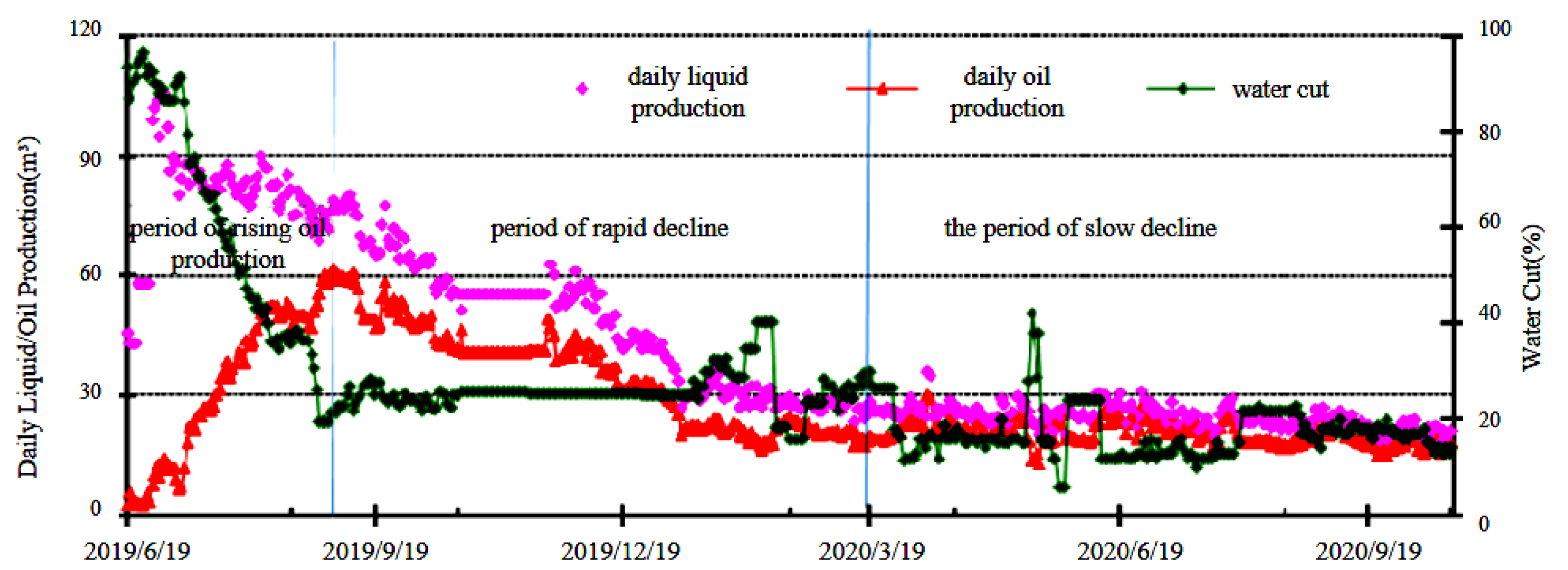
Production phases in the Jimsar shale oil reservoir: The production phases are categorized as an increase phase, a rapid decline phase, and a slow decline phase. Clarifying these production phases is crucial for developing an effective production prediction model for later stages.
(2)
Parameter optimization: By integrating and selecting data from 91 horizontal wells, the optimal range of parameters was determined, providing a deeper understanding of the production practices and extraction methods used in the Jimsar shale oil block. This highlighted that precise control over fracturing parameters is key to high productivity in the fractured horizontal wells of the Jimsar shale oil reservoir.
(3)
Guidance for fracturing optimization design: The fracturing parameters should aim to ensure a treatment volume greater than 7.21 cubic meters, a cluster spacing of less than 15.36 m, a sand volume between 2885.00 and 3356.00 cubic meters, and a segment length between 44.97 and 54.19 m.
(4)
Comparison of machine learning methods for productivity prediction: The comprehensive results indicate that the random forest algorithm is the most effective for solving productivity regression prediction problems, with data points generally falling within a 10% error margin. This study advances the application of the random forest algorithm in shale reservoir productivity prediction.

Author Contributions

Conceptualization, Y.C. (Yu Chen) and J.L.; methodology, Y.C. (Yu Chen) and S.Q.; software, Y.C. (Yu Chen); validation, Y.C. (Yu Chen) and S.Q.; formal analysis, Y.C. (Yu Chen); investigation, Y.C. (Yu Chen) and S.Q.; resources, J.L., C.L. and Y.C. (Yu Chen); data curation, Y.C. (Yu Chen); writing—original draft preparation, Y.C. (Yu Chen) and S.Q.; writing—review and editing, Y.C. (Yu Chen), J.L. and S.Q.; visualization, Y.C. (Yu Chen) and S.Q.; supervision, J.L., C.L. and Y.C. (Yiwei Chen); project administration, J.L. All authors have read and agreed to the published version of the manuscript.

Funding

This research is funded by the Major Technology Project of China Petroleum & Natural Gas Corporation (CNPC).(grant number: 2019E 26).

Data Availability Statement

Data are contained within the article.

Conflicts of Interest

Authors Chenggang Liang and Yiwei Chen were employed by the company CNPC. The remaining authors declare that the research was conducted in the absence of any commercial or financial relationships that could be construed as a potential conflict of interest. The CNPC had no role in the design of the study; in the collection, analyses, or interpretation of data; in the writing of the manuscript, or in the decision to publish the results.

References

  1. Xianwang, M.; Mei, L.; Weiqi, M.; Nie, K. Analysis of influencing factors on productivity after multistage fracturing to tight oil of horizontal well. Well Test. 2016, 25, 29–32. [Google Scholar]
  2. Zheng, D.; Miska, S.; Ozbayoglu, E.; Zhang, J. Combined Experimental and Well Log Study of Anisotropic Strength of Shale. In Proceedings of the SPE Annual Technical Conference and Exhibition, San Antonio, TX, USA, 16–18 October 2023; p. D031S046R003. [Google Scholar]
  3. Wang, Q.; Wang, T. Detection of dissolution pores in the marginally mature calcareous lucaogou shale: New insights in nanopore development in terrestrial shale oil reservoirs. Acta Geol. Sin. Engl. 2020, 94, 1321–1322. [Google Scholar] [CrossRef]
  4. Zheng, D.; Miska, S.; Ziaja, M.; Zhang, J. Study of anisotropic strength properties of shale. AGH Drill. Oil Gas 2019, 36, 93–112. [Google Scholar] [CrossRef]
  5. Chu, C.C.; Xie, Q.H. Study on capacity evaluation of fractured horizontal wells in tight gas reservoirs. CPCCS 2024, 44, 11–13. [Google Scholar]
  6. Zhiming, C.; Xinwei, L.; Chenghui, H.; Xiaoliang, Z.; Langtao, Z.; Yizhou, C.; Heng, Y. Productivity estimations for vertically fractured wells with asymmetrical multiple fractures. J. Nat. Gas Sci. Eng. 2014, 21, 1048–1060. [Google Scholar] [CrossRef]
  7. Langsrud, O. Simulation of two-phase flow by finite element methods. In Proceedings of the SPE Symposium on Numerical Simulation of Reservoir Performance, Los Angeles, CA, USA, 19–20 February 1976; p. SPE-5725-MS. [Google Scholar]
  8. Rafieepour, S.; Zheng, D.; Miska, S.; Ozbayoglu, E.; Takach, N.; Jianguo, Z. Combined Experimental and Well Log Evaluation of Anisotropic Mechanical Properties of Shales: An Application to Wellbore Stability in Bakken Formation. In Proceedings of the SPE Annual Technical Conference and Exhibition, Virtual, 26–29 October 2020; p. D021S015R006. [Google Scholar]
  9. Bai, Y.H.; Xu, B.X.; Chen, L.; Chen, G. New production prediction methods for typical curve and analytical model of shale oil and gas. China Offshore Oil Gas 2018, 30, 120–126. [Google Scholar]
  10. Li, X.C.; Li, X.P.; Jing, X.J.; Li, K. Theory and Method for Shale- Gas Productivity Analysis. Development 2014, 37, 51–55. [Google Scholar]
  11. Jing, Y. Research on Solution Method of Coupled Free Flow-Porous Media Flow Model and Reservoir Productivity Prediction Method Based on Deep Learning. Ph.D. Thesis, Shaanxi University of Science and Technology, Xian, China, 2024. [Google Scholar]
  12. Zheng, D.; Ozbayoglu, E.; Miska, S.; Zhang, J. Experimental study of anisotropic strength properties of shale. In Proceedings of the ARMA US Rock Mechanics/Geomechanics Symposium, Atlanta, GA, USA, 25–28 June 2023; p. ARMA–2023-0128. [Google Scholar]
  13. Lu, C.; Jiang, H.; Yang, J. Shale oil production prediction and fracturing optimization based on machine learning. J. Pet. Sci. Eng. 2022, 217, 110900. [Google Scholar] [CrossRef]
  14. Guo, C.J.; Wang, H.X.; Liu, X.; Zhang, C.S. An analysis of the application scenarios of machine learning technology in the oil and gas industry. China CIO News 2017, 100–103. [Google Scholar]
  15. Liu, H.; Tao, J.P.; Meng, S.W.; Li, D.X.; Cao, G.; Gao, Y. Application and prospects of CO2 enhanced oil recovery technology in shale oil reservoir. China Pet. Explor. 2022, 27, 127–134. [Google Scholar]
  16. Qian, X.; Zhang, J. Exploration and development technology of shale oil and gas in the world: Progress, impact, and implication. In Proceedings of the IOP Conference Series: Earth and Environmental Science, Changsha, China, 18–20 September 2020; p. 012131. [Google Scholar]
  17. Kuang, L.; Liu, H.; Ren, Y.; Luo, K.; Shi, M.Y.; Su, J.; LI, X. Application and development trend of artificial intelligence in petroleum exploration and development. Pet. Explor. Dev. 2020, 48, 1–11. [Google Scholar] [CrossRef]
  18. Han, D.; Jung, J.; Kwon, S. Comparative Study on Supervised Learning Models for Productivity Forecasting of Shale Reservoirs Based on a Data-Driven Approach. Appl. Sci. 2020, 10, 1267. [Google Scholar] [CrossRef]
  19. Wang, T.; Wang, Q.; Shi, J.; Zhang, W.; Ren, W.; Wang, H.; Tian, S.C. Productivity Prediction of Fractured Horizontal Well in Shale Gas Reservoirs with Machine Learning Algorithms. Appl. Sci. 2021, 11, 12064. [Google Scholar] [CrossRef]
  20. Ji, L.; Li, J.H.; Xiao, J.L. Application of random forest algorithm in the multistage fracturing stimulation of shale gas field. Pet. Geol. Oilfield Dev. Daqing 2020, 39, 168–174. [Google Scholar]
  21. Wevill, J.; Bromhead, A.; Evans, K. Relative performance of support vector machine, decision trees, and random forest classifiers for predicting production success in US unconventional shale plays. In Advances in Subsurface Data Analytics; Elsevier: Amsterdam, The Netherlands, 2022; pp. 31–62. [Google Scholar]
  22. Zheng, D.; Turhan, C.; Wang, N.; Ashok, P.; van Oort, E. Prioritizing Wells for Repurposing or Permanent Abandonment Based on Generalized Well Integrity Risk Analysis. In Proceedings of the SPE/IADC Drilling Conference and Exhibition, Galveston, TX, USA, 5–7 March 2024; p. D021S018R001. [Google Scholar]
  23. Liu, C.L.; Yang, J.; Zhu, M. Remaining life prediction method of corroded pipeline based on normal distribution. Corros 2023, 44, 100–106. [Google Scholar]
  24. Storås, A.M.; Andersen, O.E.; Lockhart, S.; Thielemann, R.; Gnesin, F.; Thambawita, V.; Hicks, S.A.; Kanters, J.K.; Strümke, I.; Halvorsen, P.J.D. Usefulness of heat map explanations for deep-learning-based electrocardiogram analysis. Diagnostics 2023, 13, 2345. [Google Scholar] [CrossRef]
  25. Wang, D.W. Application of Random Forest in Microfinance. Master’s Thesis, Chongqing University, Chongqing, China, 2019. [Google Scholar]
  26. Liu, J.L. Practice and Decision Tree Model Analysis of Comprehensive Control of “Carbon Emission” of Offshore Oilfield Torch. Tianjin Sci. Technol. 2023, 50, 40–43. [Google Scholar]
  27. Liu, F.Q.; Wang, S.Y.; Wang, M.M. Prediction of uranium reservoir permeability coefficient based on machine learning. Ore Geol. Rev. 2023, 69, 530–532. [Google Scholar]
  28. Frġedman, J. Stochastic gradient boosting. Comput. Stat. Data Anal. 2002, 38, 367–378. [Google Scholar] [CrossRef]
  29. Li, W.H.; Yang, Y.C.; Shen, H.B. Construction of Ultraviolet Radiation Fitting Model and Analysis of Correlation Factors in Guangzhou Based on Gradient Boosting Decision Tree. Meteor. Sci. Technol. 2024, 52, 124–131. [Google Scholar]
  30. Nie, Z.; Jingming, H.; Hua, C.; Guangzhao, C.; Bingyi, L. A rapid prediction method for mountain flood disaster based on machine learning algorithms. Water Resour. Prot. 2022, 38, 32–40. [Google Scholar]
  31. Junqiang, S.; Xiaoshan, L.; Shuo, W.; Kaifang, G.; Hong, P.; Xin, W. Production prediction of fractured horizontal wells in tight oil reservoirs. Xinjiang Pet. Geol. 2022, 43, 580. [Google Scholar]
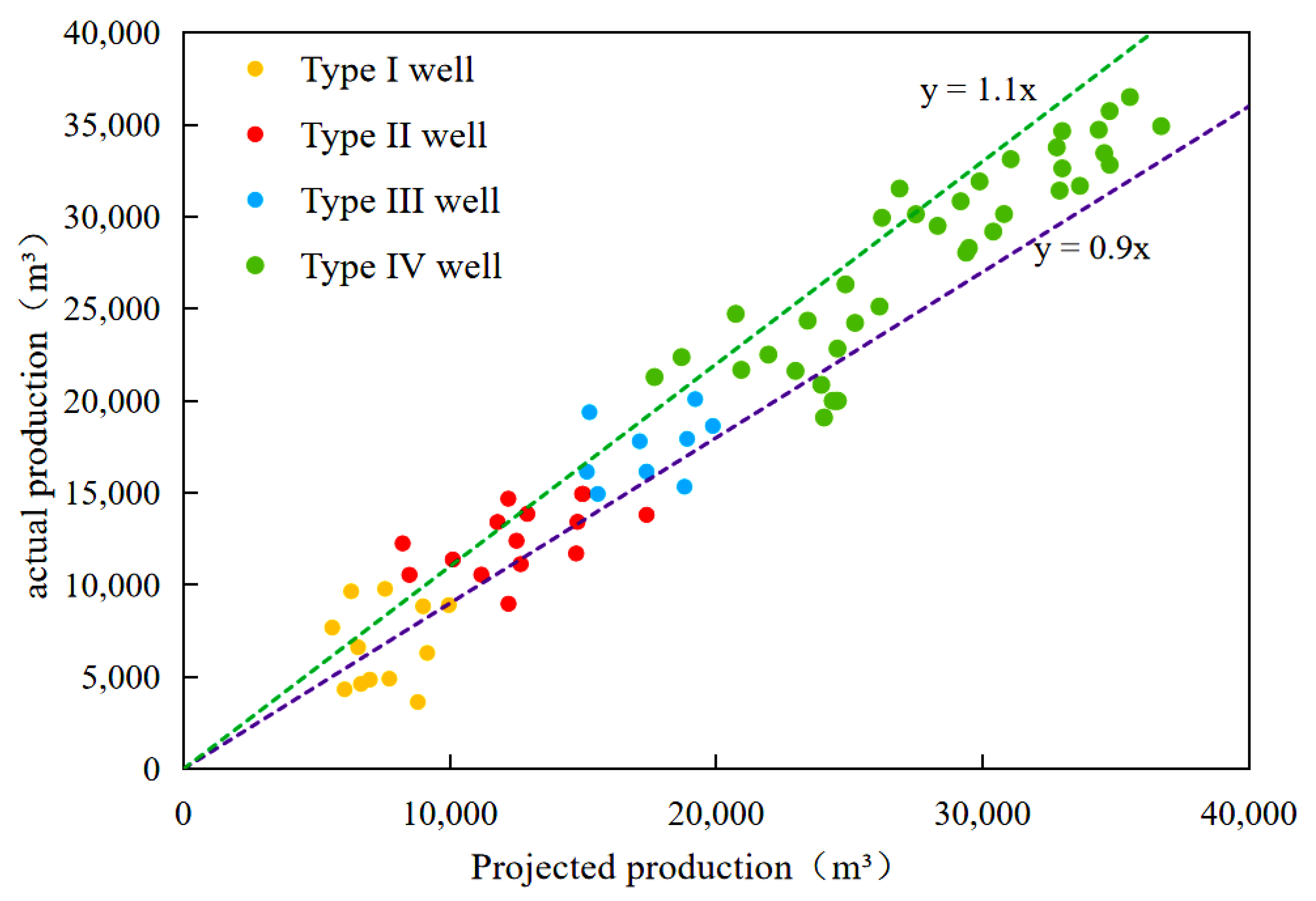
Figure 1. Characterization of production stages of horizontal wells in shale reservoirs.
Processes 12 02527 g001
Figure 2. (a) Scatter plot of oil production after 1 year compared to 3 years; (b) scatterplot of 3-year oil production vs. cumulative oil production.
Processes 12 02527 g002
Figure 3. Thermodynamic plates for shale reservoirs characterization selection.
Processes 12 02527 g003
Figure 4. Analysis of dataset properties.
Processes 12 02527 g004
Figure 5. Multivariate joint distribution plot.
Processes 12 02527 g005
Figure 6. Prediction results of three tree models.
Processes 12 02527 g006
Figure 7. Random forest model fitting.
Processes 12 02527 g007
Table 1. Classification table of development effects for shale oil horizontal wells.
ClassificationsNumber of WellsRatios (%)Oil Production over 3 Years
(104 t)
Type I well3943.50≥2
Type II well1617.401.5–2.0
Type III well2021.701.5–1.0
Type IV well1617.40≤1.0
Table 2. Characteristic parameters of fractured horizontal wells.
Characteristic ParameterRangeMean ValueStandard DeviationCharacteristic Parameter Type
Oil saturation (%)30–865210.9geologic parameter
Reservoir thickness (m)1–841.2
Porosity (%)2–1271.7
Penetration rate (103 md)0.5–3.51.80.9
Number of clusters3–1607433.6construction parameters
Cluster spacing (m)7–862625.5
Sand addition amount (m3)440–49362343934.3
Sand addition intensity (N/m2)0.6–4.01.90.5
Horizontal segment length (m)547–35001536416.0
Transformed horizontal segment length (m)231–34901251438.3
fracturing stage2–45228.5
Fracturing fluid volume (m3)7920–59,37733,189.113,874.4
Fracturing length (m)36–1195715.8
Liquid strength (N/m2)7.9–4127.39.4
Table 3. Comparison of predicted and actual capacity values for the three tree models.
Sample ValueDecision TreeRandom ForestGradient Boosting Decision TreeActual ValueSample ValueDecision TreeRandom ForestGradient Boosting Decision TreeActual Value
11005456652413215,55616,31215,90418,191
318,56216,31214,35512,32145690460085614626
512,87616,06616,97415,3686982516,31213,65911,121
78542576955617059820,32832,43235,52127,119
946588663826410,3361013,20816,31217,55314,944
1115,68316,31217,05214,8711296205634482159
13515463127856655214158898918561305
1546588122982090081612,84813,31614,63313,934
Table 4. The accuracy of the three tree models in the test set.
Model CategoryPredictive Accuracy (%)
Decision Tree70
Random Forest94
Gradient Boosted Decision Tree82
Table 5. Comparison of prediction accuracy of regression models.
Model CategoryDetermining Coefficient R2Training Set
Root Mean Square Error
Test Set
Root Mean Square Error
Decision Tree0.7960.0962.864
Random Forest0.9520.0450.934
Gradient Boosted Decision Tree0.7970.0751.232
Disclaimer/Publisher’s Note: The statements, opinions and data contained in all publications are solely those of the individual author(s) and contributor(s) and not of MDPI and/or the editor(s). MDPI and/or the editor(s) disclaim responsibility for any injury to people or property resulting from any ideas, methods, instructions or products referred to in the content.

