A Multi-Step Furnace Temperature Prediction Model for Regenerative Aluminum Smelting Based on Reversible Instance Normalization-Convolutional Neural Network-Transformer

Abstract

In the regenerative aluminum smelting process, the furnace temperature is critical for the quality and energy consumption of the product. However, the process requires protective sensors, making real-time furnace temperature measurement costly, while the strong nonlinearity and distribution drift of the process data affect furnace temperature prediction. To handle these issues, a multi-step prediction model for furnace temperature that incorporates reversible instance normalization (RevIN), convolutional neural network (CNN), and Transformer is proposed. First, the self-attention mechanism of the Transformer is combined with CNN to extract global and local information in the furnace temperature data, thus addressing the strong nonlinear characteristics of the furnace temperature. Second, RevIN with learnable affine transformation is utilized to address the distribution drift in the furnace temperature data. Third, the temporal correlation of the prediction model is enhanced by a time-coding method. The experimental results show that the proposed model demonstrates higher prediction accuracy for furnace temperature at different prediction steps in the regenerative aluminum smelting process compared to other models.

1. Introduction

Aluminum has good malleability, reflectivity, and recyclability. Based on its excellent physical and chemical properties, aluminum is widely used in the automobile, aviation, and military industries. The regenerative aluminum smelting process is an important stage for the production of aluminum, and it directly affects product quality and energy consumption [1,2]. The challenge of accurately measuring temperature is compounded by the heterogeneity of the environment in the regenerative aluminum smelting furnace and the aging of the sensors at high temperatures [3]. At present, because the real-time measurement of the furnace temperature is costly, it is common to use models to predict furnace temperature in a single step. The single-step prediction of the furnace temperature is easy to implement but sometimes does not provide sufficient information for the operators. By providing a multi-step prediction of the furnace temperature, operators have plenty of time to make adjustments compared to using a single-step prediction, resulting in increased productivity [4,5,6,7]. Therefore, researching multi-step prediction of furnace temperature is of practical significance for monitoring the state of the regenerative aluminum smelting process.

In recent years, the existing time-series prediction models have primarily been categorized into mechanism-based models, statistical models, and artificial intelligence models. Mechanism-based models require detailed analysis and simulation of the structure and production process of equipment. On this basis, mechanism-based models of industrial processes are constructed for prediction using physical or chemical principles [8]. Although mechanism-based models are characterized by strong interpretability due to their foundation in actual physical or chemical processes, the complexity of these processes often makes the construction of such models challenging. Mechanism-based models are typically reliant on idealized assumptions, which may not always hold true in practical applications, thus inevitably introducing errors that impact the accuracy of prediction results [9]. Historical features of the data are utilized by statistical models to forecast future data. Commonly used statistical models include the autoregressive model (AR) [10], autoregressive moving average model (ARMA) [11], and autoregressive integrated moving average model (ARIMA) [12]. When faced with incomplete data or data distribution drift, the accuracy of statistical models is often reduced, making it challenging to meet practical requirements [13]. With the rapid advancement of artificial intelligence technology, the research and application of artificial intelligence models in time-series prediction have garnered significant attention [14,15]. In particular, powerful tools for modeling time-series data are provided by the rise of machine learning and deep learning. The nonlinear mapping capabilities of machine learning are utilized to effectively address multivariate coupling issues within data, thus significantly improving prediction accuracy [16,17,18]. Huang et al. [19] employed kernel principal component analysis (KPCA) to extract the principal components of network inputs and optimized the extreme learning machine (ELM) using the harmony search algorithm (HS) to predict the furnace temperature in a regenerative aluminum smelting furnace. Liu et al. [20] developed a stable furnace temperature model by incorporating a restricted Boltzmann machine to enhance the stochastic initialization of input weights and hidden layer thresholds in ELM. Although multivariate coupling relationships within data are uncovered by machine learning, limitations are present in addressing the strong nonlinear characteristics of the data, resulting in prediction accuracy that often falls short of ideal levels.

With strong feature extraction and learning capabilities, deep learning is significantly superior to machine learning in processing high-dimensional data and time-series tasks [21]. Over the years, deep-learning models such as convolutional neural network (CNN), long short-term memory network (LSTM), and Transformer [22] have provided strong technical support for time-series prediction [23]. Based on deep learning, many scholars have studied the single-step prediction of time series. Duan et al. [24] proposed a single-step furnace temperature prediction model by combining working condition classification and local sample weighting LSTM. A single-step prediction model was established based on the gated recurrent unit (GRU), which used the time series of fuel and air to predict the temperature in a heating furnace [25]. A single-step prediction model for boiler temperature and oxygen content was proposed by combining CNN, bidirectional long short-term memory network (biLSTM), and squeezing and excitation (SE) network [26]. This work utilized the advantages of various deep-learning networks and significantly improved the prediction accuracy of oxygen content and boiler temperature. Ma et al. [27] proposed a single-step prediction model of temperature in an intermediate frequency furnace smelting process based on Transformer. Han et al. [28] proposed a CNN-based Transformer model that integrates the Boruta algorithm, which can effectively predict the liquefied petroleum gas output in industrial processes. By combining CNN and Transformer, local features extracted by CNN and global features captured by Transformer can be utilized to improve the accuracy of single-step prediction. These studies have provided a basic idea for the work of this paper. The advantage of these single-step prediction models is that they can maintain high prediction accuracy and stability in a short time. However, single-step prediction models often fail to effectively capture the long-term dependence in the time series, resulting in the prediction error increasing with the increase of the prediction time step. Tan et al. [29] proposed an LSTM model for the boiler of a 660 MW coal-fired power station, which effectively realized the multi-step prediction of the reheated steam temperature in the boiler. A multi-step prediction model based on Transformer is proposed for lithium-ion battery temperature [30]. The lithium-ion battery temperature, multi-step prediction model predicted 24 times more data than a single-step prediction model, and despite it having six times more running time, the prediction accuracy of the multi-step model did not decrease much. Chen et al. [31] proposed a hybrid model based on CNN and Transformer to predict ozone concentration. In the hybrid model, CNN compensates for the limited ability of Transformer to mine information from multivariable datasets, thereby improving the accuracy of multi-step prediction. However, both single-step prediction and multi-step prediction need to deal with data distribution drift in time series. Data distribution drift refers to changes in the statistical information of data over time [32]. Du et al. [33] proposed an adaptive recurrent neural network to deal with the data distribution drift of non-stationary time series. The method first characterized the data distribution information by dividing the training data into different time periods, and it then generalized the model by matching the data distribution information of these time periods. Jin et al. [34] proposed a simple and effective reversible instance normalization (RevIN) technique, which can solve the problem of data distribution drift in time series. Unlike adaptive recurrent neural networks, which were computationally expensive, RevIN was simple and effective. Although the RevIN technique has provided an important reference for this paper, the multi-step prediction of temperature for a regenerative aluminum smelting furnace, which considers both strong nonlinear characteristics and data distribution drift, cannot directly apply the results of the above research and needs further study.

Inspired by the above literature, a prediction model named RevIN-CNN-Transformer has been proposed to improve the multi-step prediction accuracy of temperature for a regenerative aluminum smelting furnace. The prediction model considers the key factors affecting furnace temperature prediction and enhances temporal correlation through time coding. The strong nonlinear characteristics and data distribution drift effects of furnace temperature data are effectively addressed through the integration of RevIN, CNN, and Transformer, resulting in accurate and stable multi-step furnace temperature predictions. The rest of this paper is structured as follows: In Section 2, the process of regenerative aluminum smelting is first introduced, and the main factors affecting furnace temperature are analyzed. In Section 3, the proposed RevIN-CNN-Transformer model is described in detail. Then, in Section 4, the proposed model is applied to furnace temperature prediction at an aluminum plant to verify its effectiveness. Finally, a summary of the entire paper is provided.

2. Regenerative Aluminum Smelting Process Analysis

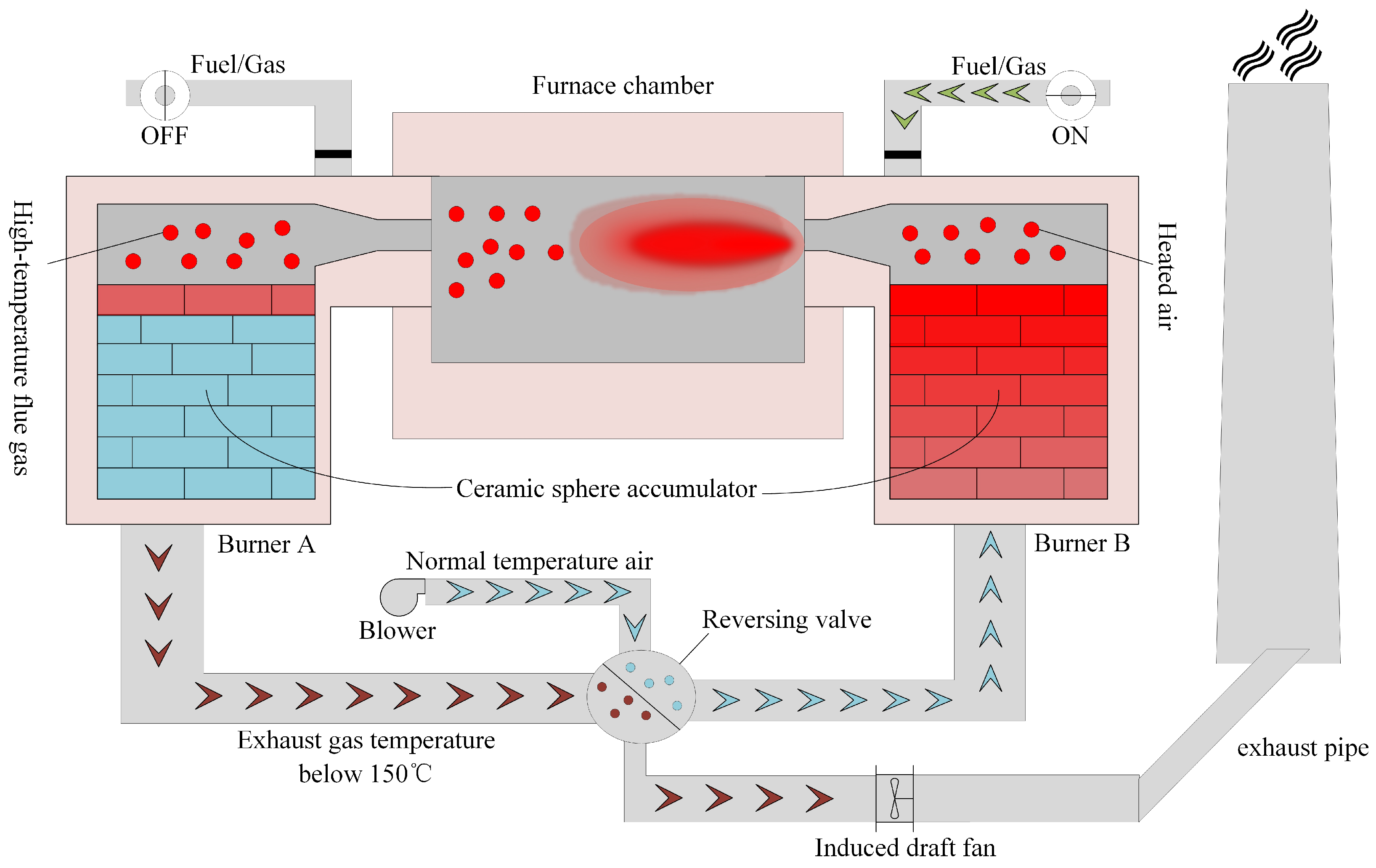
2.1. Structure and Working Principle of Regenerative Aluminum Smelting Furnace

The working process of a regenerative aluminum smelting furnace is regarded as a complex industrial process. The internal structure and operational principles of an industrial regenerative aluminum smelting furnace are illustrated in Figure 1. The regenerative aluminum smelting furnace is primarily composed of a furnace chamber, ceramic sphere accumulator, reversing valve, and exhaust pipe. The regenerative burners are arranged in pairs, with two opposing burners (A and B) forming a group. After the normal temperature air discharged from the blower enters burner B through the reversing valve, it is heated to near-furnace temperature as it passes through the ceramic sphere accumulator. After being heated, the normal temperature air enters the furnace, entraining the surrounding flue gas inside the furnace to form a high-temperature, oxygen-depleted gas stream with an oxygen content lower than 21%. The high-temperature, oxygen-depleted gas stream is mixed with the injected fuel to achieve oxygen-poor combustion of the fuel. Meanwhile, the high-temperature flue gas inside the furnace chamber is stored in the ceramic sphere accumulator and then discharged through burner A. Subsequently, an exhaust flue gas temperature below 150 °C is expelled through the reversing valve. When the heat stored in the ceramic sphere accumulator reaches saturation, the direction of the reversing valve is changed, causing burners A and B to operate alternately between combustion and heat storage states. The process of alternating between combustion and heat storage states by burners A and B is repeated cyclically, resulting in energy savings and emission reduction.

2.2. Analysis of Factors Affecting Furnace Temperature

The furnace temperature is considered a crucial index in the working process of the regenerative aluminum smelting furnace, influencing both the time and quality of aluminum smelting production. The regenerative aluminum melting process is very complex, and the furnace temperature is dynamically influenced by various factors. The main factors affecting the furnace temperature are gas flow rate, combustion air flow rate, combustion air pressure differential, combustion air valve opening, and exhaust temperature, which have a significant effect on temperature variations. Some influence on the furnace temperature is also exerted by burner switching time and combustion air temperature, but the impact is relatively small. When analyzing the factors affecting furnace temperature, burner switching time and combustion air temperature are considered secondary factors and can be ignored. Additionally, the difficulty of predicting the furnace temperature is further increased by changes in external environmental conditions and equipment aging. To better predict the furnace temperature, it is necessary that the main factors influencing the furnace temperature are analyzed in detail. Auxiliary variables affecting furnace temperature are presented in

Table 1. Auxiliary variables for furnace temperature.

Variable	Unit	Description
Gas flow rate	Nm3/h	Volume flow rate of the gas entering the furnace
Combustion air flow rate	Nm3/h	Volume flow rate of air entering the furnace for combustion
Combustion air pressure differential	Pa	The pressure differential between the air before entering the furnace and the pressure in the furnace
Combustion air valve opening	%	Valve opening for adjusting the air flow rate
Exhaust temperature	°C	Temperature of the flue gas upon exit from the furnace

. By analyzing the working principle of the regenerative aluminum smelting furnace, it can be established that the factors influencing furnace temperature are primarily comprised of two aspects.

(a) Combustion aspect: The gas flow rate and the combustion air flow rate are identified as the primary factors influencing furnace temperature. The ratio of gas flow rate to combustion air flow rate is directly influenced by the combustion efficiency. If the combustion air flow rate is excessive, the surplus air will be expelled in the form of smoke, resulting in significant heat loss and a direct reduction in furnace temperature. If the gas flow rate is excessive, insufficient combustion of the gas will be caused, and increased costs will also be incurred. The air resistance and flow entering the furnace are reflected by the combustion air pressure differential. Excessive combustion air pressure differential results in an insufficient supply of combustion air, which affects combustion efficiency and furnace temperature. On the contrary, if the combustion air pressure differential is too small, excess air is present, which increases heat loss from the furnace. The amount of air entering the furnace is determined by the combustion air valve opening. If the combustion air valve opening is too large, it can lead to excess combustion air, resulting in a significant amount of unburned gas and heat loss. On the contrary, if the combustion air valve opening is too small, insufficient air supply is experienced, leading to incomplete combustion, which affects the furnace temperature.

(b) Exhaust aspect: High-temperature flue gas is first gradually cooled by passing through the ceramic sphere regenerator, and it is then directed by the reversing valve to be discharged through the exhaust pipe. In this exhaust process, a significant amount of heat is directly removed from the furnace chamber by the high-temperature flue gas, resulting in a significant loss of energy for the process. Consequently, the exhaust temperature is considered a critical auxiliary variable in the exhaust process and must be strictly monitored and regulated to effectively reduce energy loss and improve thermal efficiency.

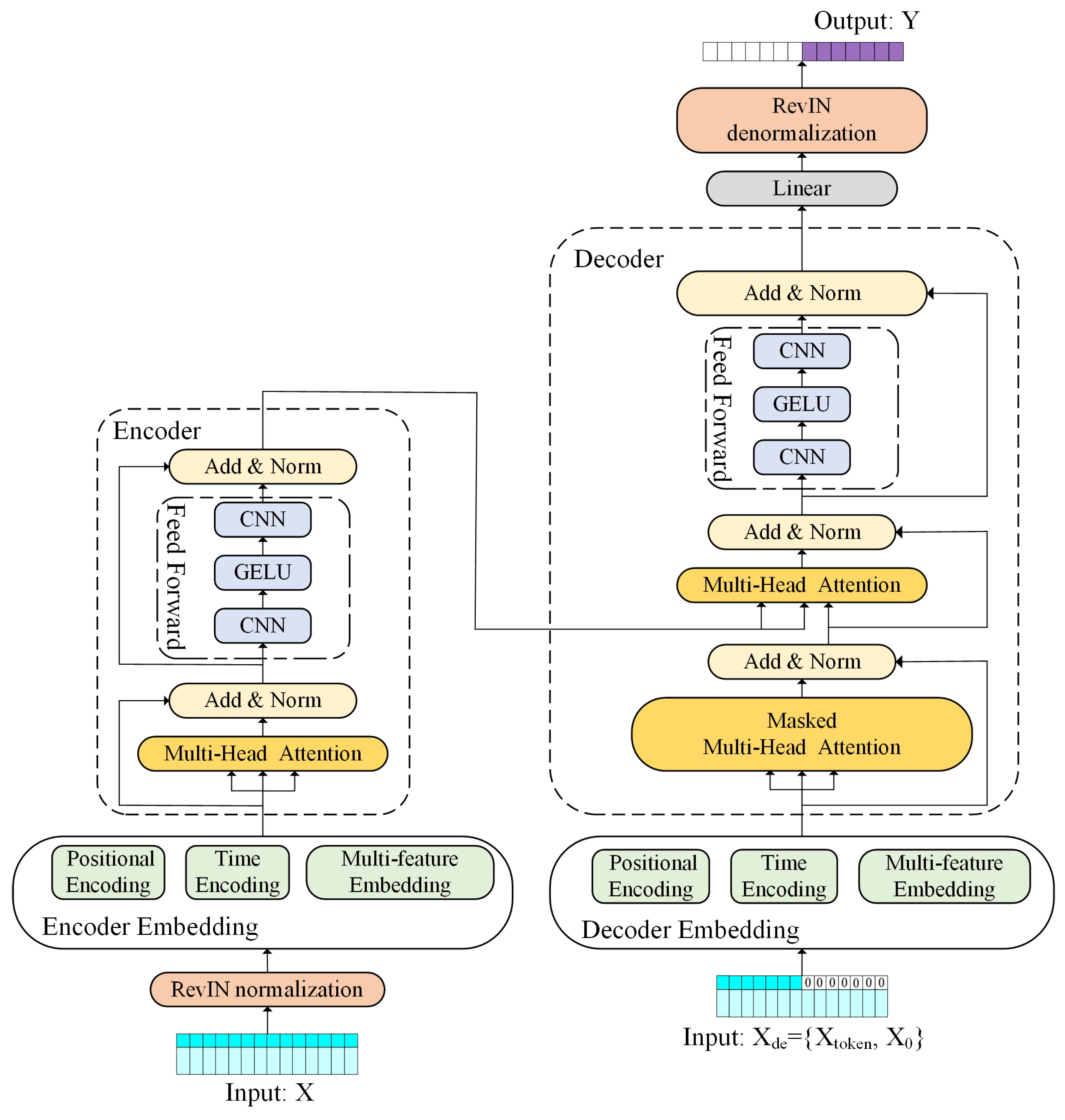
3. The RevIN-CNN-Transformer Prediction Model

To establish a multi-step prediction model for the furnace temperature in the regenerative aluminum smelting process, a RevIN-CNN-Transformer model is proposed by combining RevIN, CNN, and Transformer. Global information from the furnace temperature data is acquired through the self-attention mechanism of the Transformer, while sensitivity to local information in the furnace temperature data is improved by combining CNN. The issue of distribution drift in furnace temperature data is addressed through RevIN. Additionally, the time dependency of furnace temperature data is augmented through time coding by the proposed prediction model.

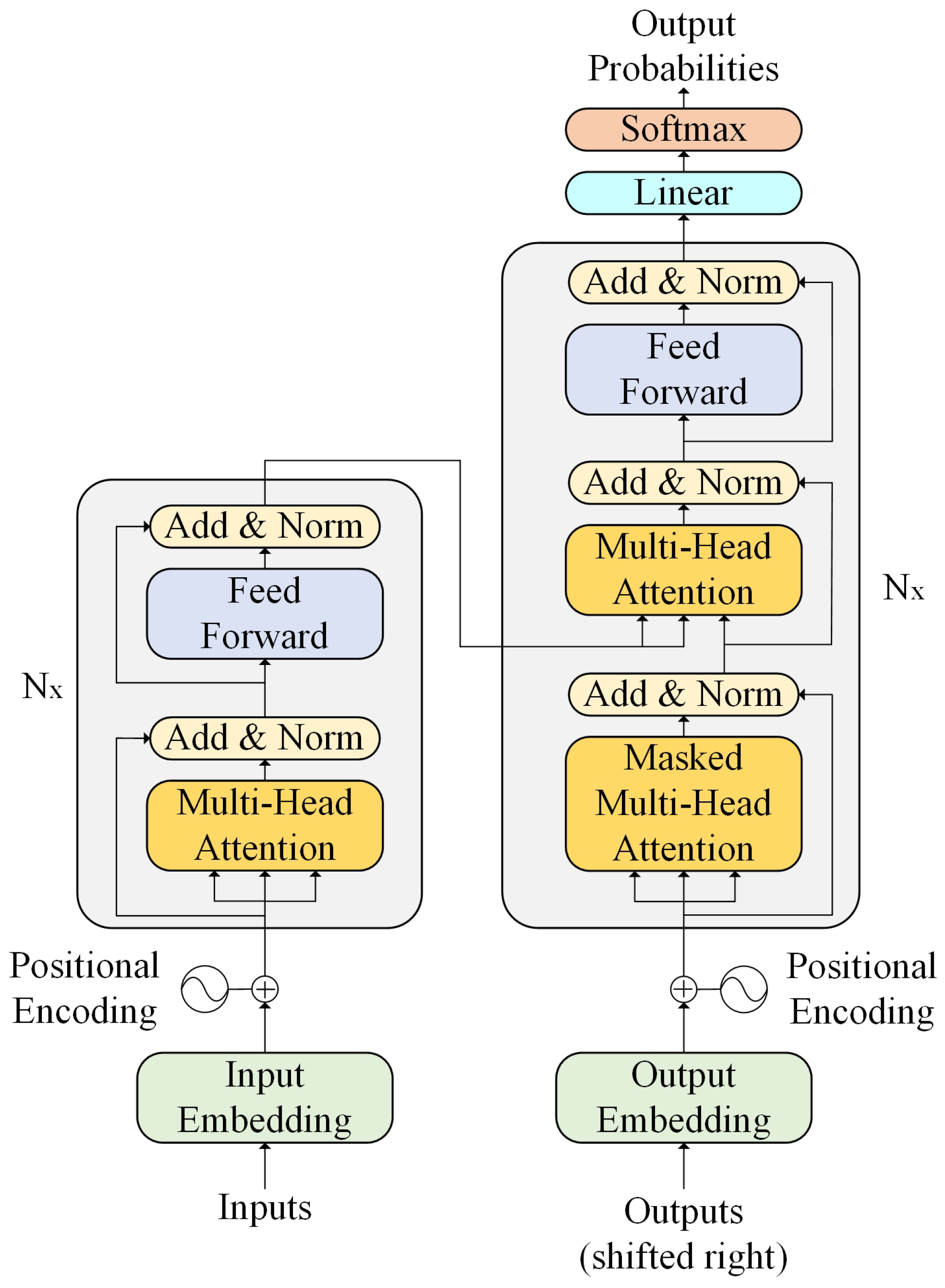
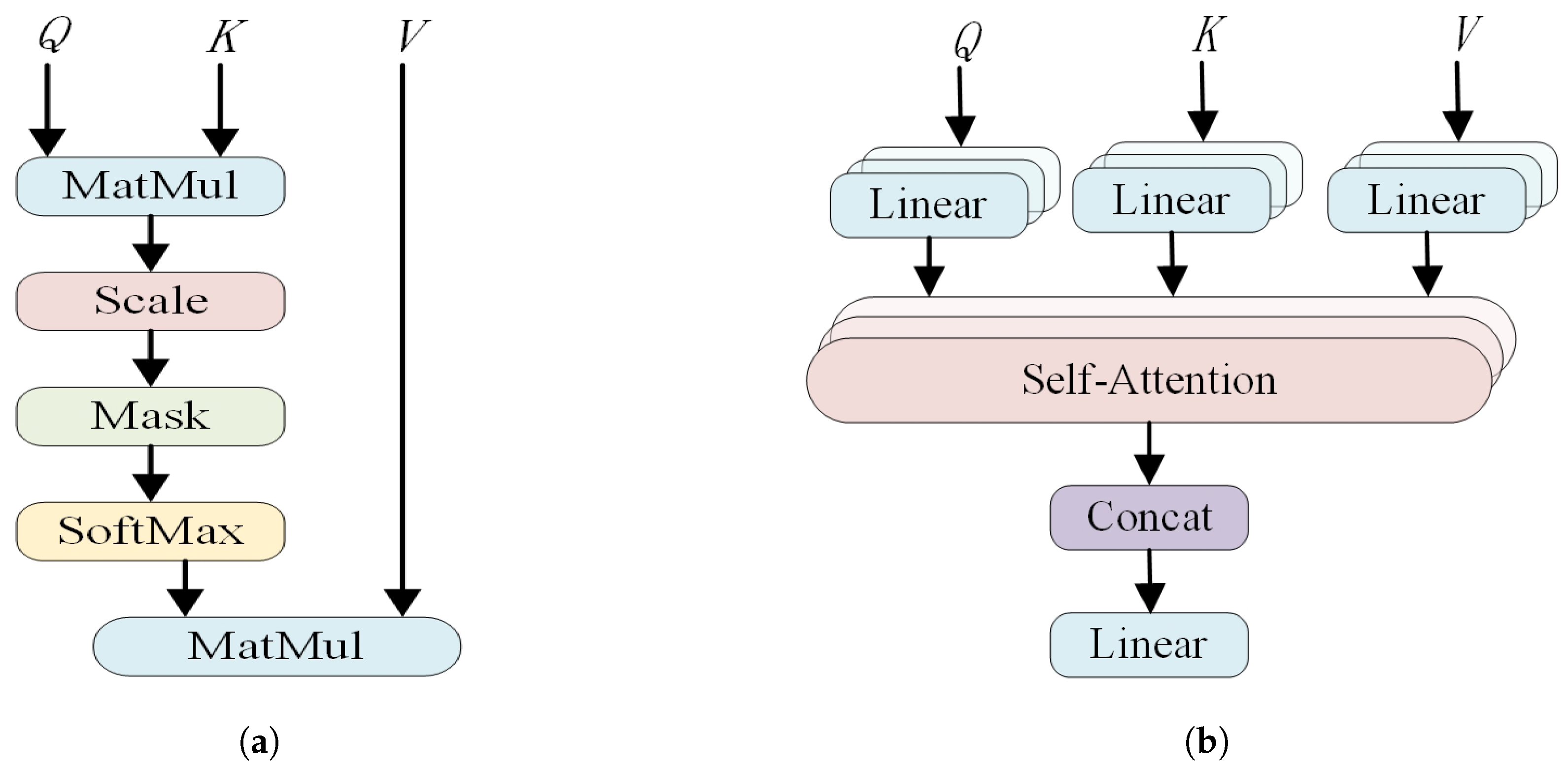
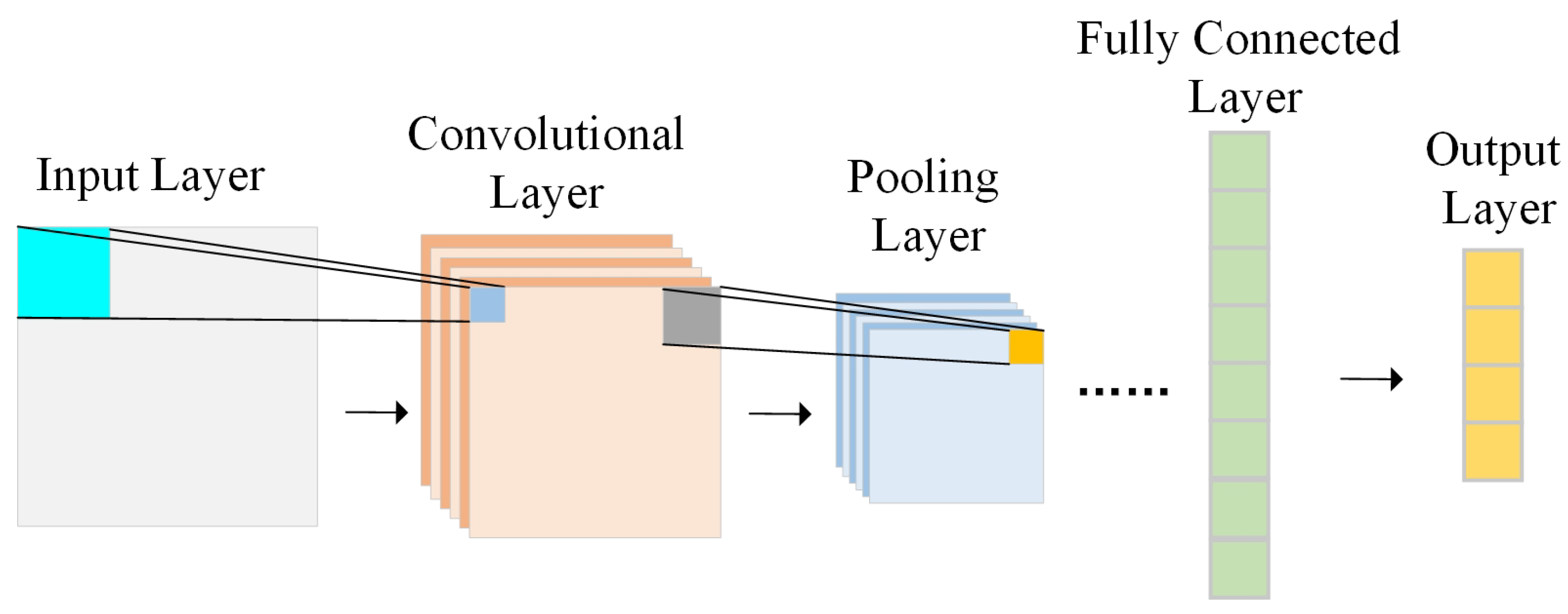
3.1. Time Coding Based CNN-Transformer

Transformer is described as a deep-learning model based on the self-attention mechanism, with the structure shown in Figure 2. Unlike traditional RNN, the recursive operations in sequence processing are discarded by the Transformer, which relies on the self-attention mechanism to handle the global dependencies of the input data. The recursive operations in sequence processing are discarded by the Transformer, with the self-attention mechanism relied upon to handle the global dependencies of the input sequence. The core structure of the Transformer model includes an encoder and a decoder, with features extracted from the input sequence by the encoder and the output generated by the decoder. The encoder is composed of multiple similar layers, each primarily consisting of a multi-head attention mechanism and a feed-forward network. The decoder is also composed of multiple similar layers, with each layer primarily including a multi-head attention mechanism, masked multi-head attention, and feed-forward network.

The self-attention mechanism is utilized by the Transformer model to handle dependencies between different positions in the input sequence, thereby allowing for better capture of long-range dependencies. The attention mechanism of the Transformer is illustrated in Figure 3. The structure of the self-attention mechanism is depicted in Figure 3a, while the structure of the multi-head attention mechanism is depicted in Figure 3b. Attention scores are calculated by the self-attention mechanism to assign weights to each position in the input sequence. The self-attention mechanism is defined as Equation (1):

$$\mathrm{Attention}\left(Q,K,V\right)=\mathrm{softmax}\left({\displaystyle \frac{Q·K^{\mathrm{T}}}{\sqrt{d_k}}}\right)·V$$

(1)

where Attention(·) is the function for self-attention calculation; $\mathit{Q}$, $\mathit{K}$, and $\mathit{V}$ are the query, key, and value matrices, respectively; T denotes the matrix transpose operation; $d_k$ denotes the dimension of the $\mathit{K}$; and softmax(·) is the normalization function used to convert scores into probabilities.

The outputs of different attention heads are concatenated by the multi-head attention mechanism, and the final multi-head attention output is obtained through linear transformations. The computation process of the multi-head attention mechanism is described as follows:

$$\mathrm{MultiHead}\left(Q,K,V\right)=\mathrm{Concat}\left({\mathrm{Head}}_1,\cdots ,{\mathrm{Head}}_h\right)·W^O$$

(2)

$${\mathrm{Head}}_i=\mathrm{Attention}\left(Q·W_i^Q,K·W_i^K,V·W_i^V\right)$$

(3)

where MultiHead(·) is the function for multi-head self-attention calculation, $\mathrm{Hea}{\mathrm{d}}_i$ denotes the output of the $\mathit{i}$ attention head, $\mathit{h}$ denotes the total number of attention heads, and Concat(·) denotes the vector concatenation operation. $W_i^Q$, $W_i^K$, and $W_i^V$ are mapping matrices used to project $\mathit{Q}$, $\mathit{K}$, and $\mathit{V}$ into a higher-dimensional representation. $W^O$ is the mapping matrix used to project the multi-head attention results back to the original lower-dimensional representation.

Compared to the self-attention mechanism, multiple subspaces are generated by the multi-head attention mechanism, allowing different aspects of the input sequence to be simultaneously attended to by the attention mechanism. Richer and more diverse features are captured in different subspaces by the multi-head attention mechanism.

Global features are captured from the input sequence by the Transformer model through the multi-head attention mechanism. However, the attention to local information within the input sequence and the perception of time-related information are found to be insufficient in the Transformer model. To more effectively extract the time-related information and local features from the furnace temperature data, embedding operations are needed. Embedding operations are comprised of positional encoding, time coding, and multi-feature embedding.

Positional information on furnace temperature data is provided by positional encoding to help the prediction model understand the relative positions of the furnace temperatures, thereby addressing the issue of lost positional information. Since time steps are not included in Transformer models as they are in RNN, positional encoding is employed to capture the relative positions of furnace temperature data. The definition of positional encoding is shown in Equation (4):

$$\left\{\begin{array}{c}PE(pos,2n)=sin\left({\displaystyle \frac{pos}{{10000}^{\frac{2n}{d_{\mathrm{model}}}}}}\right)\hfill \\ PE(pos,2n+1)=cos\left({\displaystyle \frac{pos}{{10000}^{\frac{2n}{d_{\mathrm{model}}}}}}\right)\hfill \end{array}\right.$$

(4)

where $pos$ denotes the index of the current position and n denotes the index of the dimension in the position embedding vector.

By encoding time, the ability of the prediction model to capture time-related information is significantly enhanced, leading to improved prediction accuracy. Time coding is used to convert the data from the time channel into specific time features, thus assisting the prediction model in better understanding and utilizing the time-related information within the time series. Time coding is performed by converting the time point into corresponding $minute\_number$, $hour\_number$, $day\_of\_the\_week$, and $day\_of\_the\_month$, and then scaling the values to the range [−0.5, 0.5]. The computation process of time coding is described as follows:

$$\left\{\begin{array}{c}minute\_number={\displaystyle \frac{minute}{59}}-0.5\hfill \\ hour\_number={\displaystyle \frac{hour}{23}}-0.5\hfill \\ day\_of\_week={\displaystyle \frac{weekday}{6}}-0.5\hfill \\ day\_of\_month={\displaystyle \frac{days\_passed-1}{total\_days\_in\_month-1}}-0.5\hfill \end{array}\right.$$

(5)

where $minute$ represents the number of minutes at the current time point (from 0 to 59), $hour$ represents the number of hours at the current time point (from 0 to 23), $weekday$ represents the day of the week at the current time point (from 0 to 6), and $days\_passed$ represents the day of the month at the current time point.

The CNN is used for multi-feature embedding, and the local features of furnace temperature data are able to be captured. The CNN is primarily composed of an input layer, convolutional layers, pooling layers, fully connected layers, and an output layer, and is depicted as a typical feedforward neural network, with the structure shown in Figure 4. Key information in the furnace temperature data is captured by applying convolution operations over different time periods by the CNN. Important details of furnace temperature variations are revealed through the extraction of local features by the CNN. By introducing the CNN module into the Transformer model to extract local features, the strong nonlinear characteristics of the furnace temperature data are effectively addressed, leading to an enhancement in the performance of the proposed model.

Multi-feature embedding is achieved using one-dimensional CNN, which is more suitable for furnace temperature data. The computation process of multi-feature embedding is as follows:

$$ME=Conv1d\left(X_t^N\right)$$

(6)

where $ME$ denotes the multi-feature embedding operation, $X_t^N$ denotes the one-dimensional convolution input, and $Conv1d\left(·\right)$ denotes the one-dimensional convolution operation.

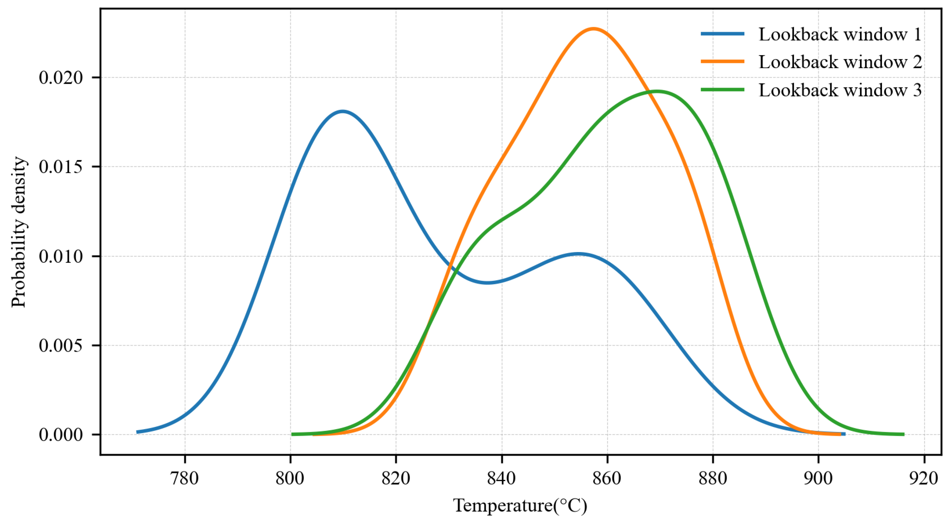
3.2. Reversible Instance Normalization

If the mean and variance, among other statistical properties, are observed to change over time in time-series data, it is an indication that a data distribution drift problem is present. The furnace temperature data, as typical time-series data, is analyzed using a window length of 30; the kernel density probability estimates for three historical windows are presented in Figure 5. It can be observed from Figure 5 that the mean and variance of the furnace temperature data are found to vary, indicating that a distribution drift problem is present in the furnace temperature data. Furnace temperature distribution drift is identified as a primary challenge hindering the accurate prediction of furnace temperature. RevIN is described as a normalization and denormalization method with learnable affine transformations, which is effectively used to address the issue of distribution drift in the data.

RevIN is composed of normalization and denormalization layers arranged in a symmetric structure. Furnace temperature prediction is treated as a multivariate time-series prediction task. Given the original input $X\in {\mathcal{R}}^{T_x\times l}$, the goal is to produce output $Y\in {\mathcal{R}}^{pre\_len\times 1}$, where $T_x$ represents the length of the input sequence, l represents the number of variables, and $pre\_len$ represents the lengths of the prediction sequences to be generated. Firstly, instance normalization is applied to the input data X. The mean and standard deviation of the input data X are computed as follows:

$$\left\{\begin{array}{c}{\mathrm{E}}_t\left[X_{lt}\right]={\displaystyle \frac{1}{T_x}}{\displaystyle \sum _{j=1}^{T_x}}{X}_{lj}\hfill \\ \mathrm{V}ar\left[X_{lt}\right]={\displaystyle \frac{1}{T_x}}{\displaystyle \sum _{j=1}^{T_x}}{(X_{lj}-{\mathrm{E}}_t\left[X_{lt}\right])}^2\hfill \end{array}\right.$$

(7)

Using these statistical measures, the input data X are normalized as Equation (8):

$${\widehat{X}}_{lt}={\gamma }_l\left({\displaystyle \frac{x_{lt}^{\left(i\right)}-{\mathrm{E}}_t\left[X_{lt}\right]}{\sqrt{\mathrm{V}ar\left[X_{lt}\right]+\epsilon }}}\right)+{\beta }_l$$

(8)

where $\gamma$ and $\beta$ denote learnable affine parameter vectors and $\epsilon$ denotes the offset.

Subsequently, the prediction model receives the instance-normalized $\widehat{X}$ as the input sequence for prediction. However, $\widehat{X}$ exhibits statistics that differ from the distribution of the original input X, and capturing the original distribution of X is challenging by merely observing the instance-normalized $\widehat{X}$. By performing denormalization at the output layer of the prediction model, the non-stationary information removed from the original input X is restored to the output of the prediction model. By applying the inverse normalization of Equation (8) to the output $\tilde{Y}$, obtained from the instance-normalized input $\widehat{X}$, which does not contain non-stationary information, the non-stationary information is restored to the final output Y of the prediction model. The process of denormalization is as follows:

$$Y=\sqrt{\mathrm{V}ar\left[X_{lt}\right]+\epsilon }·({\displaystyle \frac{\tilde{Y}-{\beta }_l}{{\gamma }_l}})+{\mathrm{E}}_t\left[X_{lt}\right]$$

(9)

where Y is the final predicted value instead of $\tilde{Y}$.

RevIN is characterized by symmetric normalization and denormalization layers, which effectively handle non-stationary information in time-series data. Non-stationary information in furnace temperature data can be removed by RevIN, and this information can be restored when needed, thus addressing the issue of distribution drift in the furnace temperature data. The application of RevIN is significant for alleviating the impact of furnace temperature data distribution drift and for improving the accuracy and stability of multi-step furnace temperature predictions.

By integrating RevIN, CNN, time coding, and Transformer, the RevIN-CNN-Transformer model is obtained. The proposed model effectively handles distribution drift in the furnace temperature data. The combination of local feature extraction by CNN and global feature extraction by Transformer is utilized to address the strong nonlinear characteristics in furnace temperature data. In addition, the temporal relevance of the proposed model is enhanced by time coding. The structure of the RevIN-CNN-Transformer model is shown in Figure 6.

The operating process of the RevIN-CNN-Transformer model is as follows:

Step 1: $X\in {\mathcal{R}}^{T_x\times l}$ is the input sequence, where $T_x$ represents the length of the input sequence and l represents the number of variables. By applying RevIN normalization to X through Equation (8), $E\left(X\right)$ is obtained.

Step 2: Perform Encoder Embedding operation on $E\left(X\right)$.

(a)

By applying positional encoding to $E\left(X\right)$ through Equation (4), $PE\left(X\right)\in {\mathcal{R}}^{T_x\times d_{model}}$ is obtained, where $d_{model}$ represents the dimensions of the prediction model.

(b)

By applying time coding to $E\left(X\right)$ through Equation (5), $TE\left(X\right)\in {\mathcal{R}}^{T_x\times d_{model}}$ is obtained.

(c)

By applying multi-feature embedding to $E\left(X\right)$ through Equation (6), $ME\left(X\right)\in {\mathcal{R}}^{T_x\times d_{model}}$ is obtained.

Then, by summing $PE\left(X\right)$, $TE\left(X\right)$, and $ME\left(X\right)$, $Z_0=PE\left(X\right)+TE\left(X\right)+ME\left(X\right)$ is obtained.

Step 3: By applying the multi-head attention mechanism to $Z_0$, $Z_N=\mathrm{MultiHead}(Z_0)\in {\mathcal{R}}^{T_x\times d_{model}}$ is obtained.

Step 4: After passing $Z_N$ through the feedforward network, the output of the encoder is $Z_N^{\prime }=\mathrm{GELU}(Conv1d(Z_N))\in {\mathcal{R}}^{T_x\times d_{model}}$.

Step 5: $X_{token}\in {\mathcal{R}}^{Label\_len\times l}$, where $Label\_len$ represents the lengths of known data used by the decoder during the prediction process. $X_0\in {\mathcal{R}}^{pre\_len\times l}$, where $pre\_len$ represents the lengths of the prediction sequences to be generated. Therefore, the input to the decoder is $X_{de}=\left\{X_{token},X_0\right\}\in {\mathcal{R}}^{T_y\times l}$, and $T_y=Label\_len+pre\_len$ represents the length of the target sequence fed into the decoder.

Step 6: Perform decoder embedding operation on $X_{de}$.

(a)

By applying positional encoding to $X_{de}$ through Equation (4), $P{X}_{de}\in {\mathcal{R}}^{T_y\times d_{model}}$ is obtained.

(b)

By applying time coding to $X_{de}$ through Equation (5), $T{X}_{de}\in {\mathcal{R}}^{T_y\times d_{model}}$ is obtained.

(c)

By applying multi-feature embedding to $X_{de}$ through Equation (6), $M{X}_{de}\in {\mathcal{R}}^{T_y\times d_{model}}$ is obtained.

Then, by summing $P{X}_{de}$, $T{X}_{de}$, and $M{X}_{de}$, $Z_0^{\prime }=P{X}_{de}+T{X}_{de}+M{X}_{de}$ is obtained.

Step 7: By applying masked multi-head attention to $Z_0^{\prime }$, $Z_w^{\prime }=\mathrm{MultiHead}(Z_0^{\prime })\in {\mathcal{R}}^{T_y\times d_{model}}$ is obtained.

Step 8: By combining the encoder’s output, $Z_w^{\prime }$ passes through the encoder–decoder attention, yielding $Z_w^{″}=\mathrm{MultiHead}(Z_w^{\prime },Z_N^{\prime })\in {\mathcal{R}}^{T_y\times d_{model}}$.

Step 9: After passing $Z_w^{″}$ through the feedforward network, the output of the decoder is $Z_N^{″}=\mathrm{GELU}(Conv1d(Z_w^{″}))\in {\mathcal{R}}^{T_y\times d_{model}}$.

Step 10: After passing $Z_N^{″}$ through the linear layer and then applying RevIN denormalization, the final output $Y\in {\mathcal{R}}^{pre\_len\times 1}$ is obtained.

4. Industrial Case

4.1. Dataset and Data Preprocessing

In order to verify the performance of the RevIN-CNN-Transformer model, it was applied to the multi-step prediction of furnace temperature in an industrial regenerative aluminum smelting plant. The aluminum plant was characterized by high-temperature smelting and a complex production process, with advanced technology and equipment utilized for large-scale aluminum production. Through the mechanistic analysis of the regenerative aluminum melting furnace, it is found that seven factors influence the furnace temperature. However, during the data collection, the variations in burner switching time and combustion air temperature are relatively small. Therefore, the influence of burner switching time and combustion air temperature is ignored during the prediction of furnace temperature. To construct the model, the selected auxiliary variables are shown in

Table 2. Auxiliary variables of the proposed model.

Index	Auxiliary Variable
1	12 # Gas flow rate
2	34 # Gas flow rate
3	12 # Combustion air flow rate
4	34 # Combustion air flow rate
5	12 # Combustion air pressure differential
6	34 # Combustion air pressure differential
7	12 # Combustion air valve opening
8	34 # Combustion air valve opening
9	B3 # Exhaust temperature

. These auxiliary variables are measured by sensors. The types and parameters of the sensors are shown in

Table 3. Sensor types and parameters.

Sensor Type	Measurement Range	Accuracy	Response Time
Flow Meter	0–15 m3/h	±1%	0.2 s
Differential Pressure Gauge	0–10,000 Pa	±0.5%	0.1 s
Valve Position Indicator	0–100%	±1%	0.1 s
Thermocouple	0–1200 °C	±0.5%	0.5 s

. The data were collected from the regenerative aluminum smelting furnace in the plant, spanning from 1 November to 29 November 2017. The data were sampled every 5 min, resulting in a dataset of 8000 samples. The dataset was divided as follows: 80% of the data were allocated to the training set, 10% to the validation set, and the remaining 10% to the test set. The comprehensive assessment of the performance of the RevIN-CNN-Transformer model in furnace temperature prediction was enabled by the division of the dataset.

To eliminate the impact caused by differences in dimensions among variables and enable comparison on the same scale, standardization is performed. Z-score standardization is employed in this paper, with the specific expression in Equation (10):

$$x_i^{*}={\displaystyle \frac{x_i-\mu }{\sigma }}$$

(10)

where $x_i$ denotes the original data value, $\mu$ denotes the mean of the data, $\sigma$ denotes the standard deviation of the data, and $x_i^{*}$ denotes the standardized value.

To evaluate the performance of the proposed prediction model, the root mean squared error (RMSE), the mean absolute error (MAE), and the coefficient of determination (R²) are selected as evaluation indices. Smaller values of RMSE and MAE are associated with higher prediction accuracy. Greater accuracy in the prediction results is indicated by a value of R² closer to 1. The three evaluation indices are defined as follows:

$$RMSE=\sqrt{{\displaystyle \frac{1}{N_T}}\sum _{i=1}^{N_T}{(y_i-{\widehat{y}}_i)}^2}$$

(11)

$$MAE={\displaystyle \frac{1}{N_T}}\sum _{i=1}^{N_T}\left|y_i-{\widehat{y}}_i\right|$$

(12)

$$R^2=1-{\displaystyle \frac{{\displaystyle \sum _{i=1}^{N_T}}{(y_i-{\widehat{y}}_i)}^2}{{\displaystyle \sum _{i=1}^{N_T}}{(y_i-\overline{y})}^2}}$$

(13)

where $N_T$ denotes the number of samples used for testing, $y_i$ denotes the actual value of the furnace temperature, ${\widehat{y}}_i$ denotes the predicted value of the furnace temperature, and ${\overline{y}}_i$ denotes the mean value of the actual furnace temperature.

4.2. Results and Analysis

The experiments in this paper are run on the Windows 11 operating system, configured with an Intel(R) Core(TM) i5-12490F CPU and a GeForce RTX 4060 GPU. The experimental environment uses the Pytorch framework, and Python version 3.10.13 is installed. Hyperparameters such as learning rate, epoch, and batch size are shown to have a significant impact on the performance of the prediction model; therefore, optimal settings are necessary. The learning rate is identified as one of the key hyperparameters that need to be adjusted during the training of the prediction model. A learning rate that is too high may prevent convergence and cause oscillations, while a rate that is too low may slow convergence and waste training time. The performance metrics of the prediction model under different learning rates can be obtained through the trial and error method, as shown in

Table 4. Model performance at different learning rates.

Learning Rate	MAE	RMSE	R2
0.01	44.612	52.854	0.415
0.001	2.487	3.570	0.997
0.0001	1.984	2.865	0.998
0.00001	3.041	4.188	0.996

. From Table 4, it is shown that the optimal learning rate for the proposed model should be set to 0.0001. The optimal settings for the two hyperparameters, epoch and batch size, are also found through the trial and error method, with optimal values being 15 and 12, respectively.

The loss function adopted by the proposed model is the mean squared error (MSE). Under the optimal settings of hyperparameters, the loss curves for the training and validation sets are shown in Figure 7. It can be observed from Figure 7 that the loss curves for both the training and validation sets tend to stabilize after a certain number of iterations, indicating that the errors of the prediction model on the training and validation sets are stabilized at a lower level. The error of the prediction model tends to zero and stabilizes, demonstrating that the prediction model converges.

To comprehensively evaluate the performance of the proposed model, comparative experiments and ablation experiments are conducted. The comparative experiments are primarily used to assess the performance advantages of the proposed model relative to some existing deep-learning models. The ablation experiments are used to analyze the contribution of each component of the proposed prediction model to the overall performance.

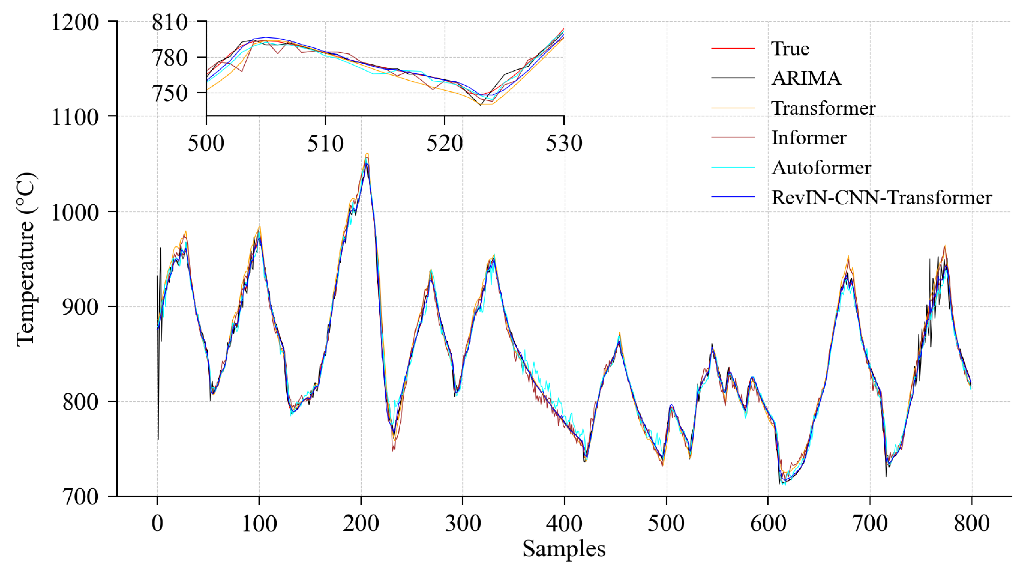
4.2.1. Comparative Experiments

To verify the superiority of the proposed model, the ARIMA model, the Transformer model [22], the Informer model [35], and the Autoformer model [36] are used for experimental comparison. The performances of the RevIN-CNN-Transformer model, the ARIMA model, the Transformer model, the Informer model, and the Autoformer model are compared in the furnace temperature prediction task with 1-step, 4-step, and 8-step prediction steps. The prediction results of the five models with 1-step, 4-step, and 8-step prediction steps are shown in Figure 8, Figure 9, and Figure 10, respectively.

In a magnified view of the prediction results from Figure 8, the prediction curve of the RevIN-CNN-Transformer model is shown to fit the actual values accurately and to follow the fluctuations of the actual curve closely. As shown in Figure 9 and Figure 10, the decrease in the performances of the five models as the prediction step increases and the increase in the fluctuation of the prediction curves are observed. However, the prediction results of the RevIN-CNN-Transformer model are significantly better than those of the other prediction models. The comparative experimental results demonstrate that better performance is achieved by the RevIN-CNN-Transformer model in the multi-step furnace temperature prediction task. The evaluation index results for the five models at 1-step, 4-step, and 8-step furnace temperature prediction steps are shown in

Table 5. The results of the evaluation indices for the models under different prediction steps.

Prediction Step	Evaluation Metrics	ARIMA	Transformer	Informer	Autoformer	RevIN-CNN-Transformer
1-step	MAE	3.181	6.312	6.061	5.107	1.984
	RMSE	7.592	8.283	7.810	6.889	2.865
	R2	0.988	0.986	0.987	0.990	0.998
4-step	MAE	8.063	9.648	8.691	8.897	5.755
	RMSE	16.249	12.126	11.849	11.892	8.351
	R2	0.949	0.969	0.971	0.970	0.985
8-step	MAE	18.376	14.872	12.129	19.943	10.600
	RMSE	32.735	19.112	16.766	27.491	15.998
	R2	0.810	0.924	0.941	0.842	0.946

.

It can be seen from Table 5 that the RevIN-CNN-Transformer model performs better than the other four prediction models across the three prediction steps. Among the three prediction steps, the smallest values of MAE and RMSE and the highest value of R² are exhibited by the RevIN-CNN-Transformer model, indicating that higher prediction accuracy and better fitting performance are achieved by the proposed model.

The comparison of the reduction rates of MAE and RMSE for the other four prediction models relative to the RevIN-CNN-Transformer model under 1-step, 4-step, and 8-step prediction steps is shown in Figure 11.

The better prediction performance of the RevIN-CNN-Transformer model compared to the other prediction models for 1-step, 4-step, and 8-step prediction steps is shown in Figure 11. In the 1-step prediction, reductions of 38 to 69% in MAE and 58 to 65% in RMSE are achieved by the RevIN-CNN-Transformer model. In the 4-step prediction, reductions of 29 to 40% in MAE and 30 to 49% in RMSE are achieved by the proposed model. In the 8-step prediction, the proposed model achieves reductions of 13 to 47% in MAE and 5 to 51% in RMSE. The RevIN-CNN-Transformer model has smaller MAE and RMSE values compared to the other four prediction models, indicating that smaller prediction errors, lower dispersion, and better prediction performance are obtained.

4.2.2. Ablation Experiments

To validate the effectiveness of each component in the proposed prediction model, systematic ablation experiments are conducted. The impact of removing key components of the prediction model on prediction performance is assessed. All ablation experiments are conducted on the same dataset with the same training parameters. The evaluation indices of MAE, RMSE, and R² are used to ensure the comparability of the ablation experiment results. The CNN and RevIN are added separately to the Transformer model to explore their effects. The impact of removing the time-coding module from the RevIN-CNN-Transformer model is analyzed. All ablation experiments are conducted on the furnace temperature prediction task with a 4-step prediction horizon, and the results are shown in Figure 12.

The evaluation indices of the ablation experiments for the RevIN-CNN-Transformer model are presented in

Table 6. The results of the evaluation indices for the ablation experiments of the prediction model.

Prediction Model	MAE	RMSE	R2
CNN-Transformer	8.118	10.681	0.976
RevIN-Transformer	6.856	9.743	0.980
RevIN-CNN-Transformer (without time coding)	6.317	9.268	0.982
RevIN-CNN-Transformer	5.755	8.351	0.985

.

It can be seen from Table 6 that the performance of the RevIN-CNN-Transformer model is significantly improved by the introduction of the CNN and RevIN modules. Specifically, the issue of distribution drift in the furnace temperature data is effectively addressed by the RevIN module. The ability of the RevIN-CNN-Transformer model to focus on local information is enhanced by the CNN module through the extraction of local features from the furnace temperature data. The RevIN-CNN-Transformer model is enabled to better understand the overall trend of the furnace temperature and effectively capture the details within the temperature data through the introduction of the CNN and RevIN modules, thus improving the accuracy and stability of the predictions. Additionally, the temporal correlation of the RevIN-CNN-Transformer model is enhanced by the time-coding module. The performance of the proposed model in handling complex and multivariate coupling furnace temperature prediction tasks is significantly improved by the combination of the Transformer, CNN, RevIN, and time-coding modules.

5. Conclusions

A multi-step furnace temperature prediction model based on RevIN-CNN-Transformer is proposed to address the issues of strong nonlinear characteristics and distribution drift of furnace temperature for the regenerative aluminum melting process. The ability of the predictive model to learn time-related information is significantly enhanced by applying time coding to the input data. A significant improvement in the furnace temperature prediction is achieved by the proposed model, which utilizes the local feature extraction capabilities of CNN and the global feature extraction capabilities of Transformer. In addition, the issue of decreased prediction performance due to data distribution drift is effectively addressed by the introduction of RevIN. The experimental results from the furnace temperature dataset of an aluminum smelting plant show that time-related information is effectively extracted from the furnace temperature data by the proposed model. The proposed model surpasses the evaluation indices of the other models for multi-step prediction. The strong nonlinear characteristics and distribution drift issues of furnace temperature are addressed by the proposed prediction model, and favorable application results are achieved in the multi-step furnace temperature prediction. Compared to single-step prediction, multi-step prediction provides operators with more long-term predictive information, allowing them sufficient time to make adjustments, thereby improving production efficiency and reducing energy consumption. Although the errors of multi-step prediction may accumulate as the number of prediction steps increases, the opportunity for operators to have sufficient time for adjustments holds practical significance in industrial applications.

References

1. Qiu, L.; Feng, Y.; Chen, Z.; Li, Y.; Zhang, X. Numerical simulation and optimization of the melting process for the regenerative aluminum melting furnace. Appl. Therm. Eng. 2018, 145, 315–327. [Google Scholar] [CrossRef]
2. Bozkurt, Ö.; Kaya, M.F. A CFD Assisted Study: Investigation of the Transformation of A Recuperative Furnace to Regenerative Furnace For Industrial Aluminium Melting. Eng. Mach. Mag. 2021, 62, 245–261. [Google Scholar] [CrossRef]
3. Chen, X.; Dai, J.; Luo, Y. Temperature prediction model for a regenerative aluminum smelting furnace by a just-in-time learning-based triple-weighted regularized extreme learning machine. Processes 2022, 10, 1972. [Google Scholar] [CrossRef]
4. Yin, L.; Zhou, H. Modal decomposition integrated model for ultra-supercritical coal-fired power plant reheater tube temperature multi-step prediction. Energy 2024, 292, 130521. [Google Scholar] [CrossRef]
5. Xue, P.; Jiang, Y.; Zhou, Z.; Chen, X.; Fang, X.; Liu, J. Multi-step ahead forecasting of heat load in district heating systems using machine learning algorithms. Energy 2019, 188, 116085. [Google Scholar] [CrossRef]
6. Khosravi, K.; Golkarian, A.; Barzegar, R.; Aalami, M.T.; Heddam, S.; Omidvar, E.; Keesstra, S.D.; López-Vicente, M. Multi-step ahead soil temperature forecasting at different depths based on meteorological data: Integrating resampling algorithms and machine learning models. Pedosphere 2023, 33, 479–495. [Google Scholar] [CrossRef]
7. Zhao, Y.; Ma, Z.; Han, X. Research on multi-step mixed predictiom model of coal gasifier furnace temperature based on machine learning. Proc. J. D Conf. Ser. 2022, 2187, 012070. [Google Scholar] [CrossRef]
8. Yan, M.; Bi, H.; Wang, H.; Xu, C.; Chen, L.; Zhang, L.; Chen, S.; Xu, X.; Chen, Q.; Jia, Y.; et al. Advanced soft-sensing techniques for predicting furnace temperature in industrial organic waste gasification. Process. Saf. Environ. Prot. 2024, 190, 1253–1262. [Google Scholar] [CrossRef]
9. Dai, J.; Chen, N.; Yuan, X.; Gui, W.; Luo, L. Temperature prediction for roller kiln based on hybrid first-principle model and data-driven MW-DLWKPCR model. ISA Trans. 2020, 98, 403–417. [Google Scholar] [CrossRef]
10. Rasul, K.; Seward, C.; Schuster, I.; Vollgraf, R. Autoregressive denoising diffusion models for multivariate probabilistic time series forecasting. In Proceedings of the 38th International Conference on Machine Learning, Online, 18–24 July 2021; Volume 139, pp. 8857–8868. [Google Scholar]
11. Magadum, R.B.; Bilagi, S.; Bhandarkar, S.; Patil, A.; Joshi, A. Short-term wind power forecast using time series analysis: Auto-regressive moving-average model (ARMA). In Recent Developments in Electrical and Electronics Engineering: Select Proceedings of ICRDEEE 2022; Springer: Singapore, 2023; Volume 979, pp. 319–341. [Google Scholar]
12. Kumar, R.; Kumar, P.; Kumar, Y. Multi-step time series analysis and forecasting strategy using ARIMA and evolutionary algorithms. Int. J. Inf. Technol. 2022, 14, 359–373. [Google Scholar] [CrossRef]
13. Lin, W.; Zhang, B.; Li, H.; Lu, R. Multi-step prediction of photovoltaic power based on two-stage decomposition and BILSTM. Neurocomputing 2022, 504, 56–67. [Google Scholar] [CrossRef]
14. Wang, Y.; Xu, Y.; Song, X.; Sun, Q.; Zhang, J.; Liu, Z. Novel method for temperature prediction in rotary kiln process through machine learning and CFD. Powder Technol. 2024, 439, 119649. [Google Scholar] [CrossRef]
15. Kong, X.; Du, X.; Xue, G.; Xu, Z. Multi-step short-term solar radiation prediction based on empirical mode decomposition and gated recurrent unit optimized via an attention mechanism. Energy 2023, 282, 128825. [Google Scholar] [CrossRef]
16. Hu, Y.; Man, Y.; Ren, J.; Zhou, J.; Zeng, Z. Multi-step carbon emissions forecasting model for industrial process based on a new strategy and machine learning methods. Process. Saf. Environ. Prot. 2024, 187, 1213–1233. [Google Scholar] [CrossRef]
17. Aljuaydi, F.; Wiwatanapataphee, B.; Wu, Y.H. Multivariate machine learning-based prediction models of freeway traffic flow under non-recurrent events. Alex. Eng. J. 2023, 65, 151–162. [Google Scholar] [CrossRef]
18. Feng, K.; Yang, L.; Su, B.; Feng, W.; Wang, L. An integration model for converter molten steel end temperature prediction based on Bayesian formula. Steel Res. Int. 2022, 93, 2100433. [Google Scholar] [CrossRef]
19. Huang, Q.; Lei, S.; Jiang, C.; Xu, C. Furnace temperature prediction of aluminum smelting furnace based on KPCA-ELM. In Proceedings of the 2018 Chinese Automation Congress (CAC), Xi’an, China, 30 November–2 December 2018; pp. 1454–1459. [Google Scholar]
20. Liu, Q.; Wei, J.; Lei, S.; Huang, Q.; Zhang, M.; Zhou, X. Temperature prediction modeling and control parameter optimization based on data driven. In Proceedings of the 2020 IEEE Fifth International Conference on Data Science in Cyberspace (DSC), Hong Kong, China, 27–30 July 2020; pp. 8–14. [Google Scholar]
21. Zhang, Z.; Dai, H.; Jiang, D.; Yu, Y.; Tian, R. Multi-step ahead forecasting of wind vector for multiple wind turbines based on new deep learning model. Energy 2024, 304, 131964. [Google Scholar] [CrossRef]
22. Vaswani, A.; Shazeer, N.; Parmar, N.; Uszkoreit, J.; Jones, L.; Gomez, A.N.; Kaiser, L.; Polosukhin, I. Attention is all you need. In Proceedings of the 31st International Conference on Neural Information Processing Systems, Long Beach, CA, USA, 4–9 December 2017; pp. 6000–6010. [Google Scholar]
23. Dettori, S.; Matino, I.; Colla, V.; Speets, R. A deep-learning-based approach for forecasting off-gas production and consumption in the blast furnace. Neural Comput. Appl. 2022, 34, 911–923. [Google Scholar] [CrossRef]
24. Duan, Y.; Dai, J.; Luo, Y.; Chen, G.; Cai, X. A Dynamic Time Warping Based Locally Weighted LSTM Modeling for Temperature Prediction of Recycled Aluminum Smelting. IEEE Access 2023, 11, 36980–36992. [Google Scholar] [CrossRef]
25. Chen, C.J.; Chou, F.I.; Chou, J.H. Temperature prediction for reheating furnace by gated recurrent unit approach. IEEE Access 2022, 10, 33362–33369. [Google Scholar] [CrossRef]
26. Ji, Z.; Tao, W.; Ren, J. Boiler furnace temperature and oxygen content prediction based on hybrid CNN, biLSTM, and SE-Net models. Appl. Intell. 2024, 54, 8241–8261. [Google Scholar] [CrossRef]
27. Ma, S.; Li, Y.; Luo, D.; Song, T. Temperature Prediction of Medium Frequency Furnace Based on Transformer Model. In Proceedings of the International Conference on Neural Computing for Advanced Applications, Jinan, China, 8–10 July 2022; Volume 1637, pp. 463–476. [Google Scholar]
28. Han, Y.; Han, L.; Shi, X.; Li, J.; Huang, X.; Hu, X.; Chu, C.; Geng, Z. Novel CNN-based transformer integrating Boruta algorithm for production prediction modeling and energy saving of industrial processes. Expert Syst. Appl. 2024, 255, 124447. [Google Scholar] [CrossRef]
29. Tan, P.; Zhu, H.; He, Z.; Jin, Z.; Zhang, C.; Fang, Q.; Chen, G. Multi-step ahead prediction of reheat steam temperature of a 660 MW coal-fired utility boiler using long short-term memory. Front. Energy Res. 2022, 10, 845328. [Google Scholar] [CrossRef]
30. Wan, Z.; Kang, Y.; Ou, R.; Xue, S.; Xu, D.; Luo, X. Multi-step time series forecasting on the temperature of lithium-ion batteries. J. Energy Storage 2023, 64, 107092. [Google Scholar] [CrossRef]
31. Chen, Y.; Chen, X.; Xu, A.; Sun, Q.; Peng, X. A hybrid CNN-Transformer model for ozone concentration prediction. Air Qual. Atmos. Health 2022, 15, 1533–1546. [Google Scholar] [CrossRef]
32. Fan, W.; Wang, P.; Wang, D.; Wang, D.; Zhou, Y.; Fu, Y. Dish-ts: A general paradigm for alleviating distribution shift in time series forecasting. In Proceedings of the AAAI Conference on Artificial Intelligence, Washington, DC, USA, 7–14 February 2023; Volume 37, pp. 7522–7529. [Google Scholar]
33. Du, Y.; Wang, J.; Feng, W.; Pan, S.; Qin, T.; Xu, R.; Wang, C. Adarnn: Adaptive learning and forecasting of time series. In Proceedings of the 30th ACM International Conference on Information & Knowledge Management, Queensland, Australia, 1–5 November 2021; pp. 402–411. [Google Scholar]
34. Kim, T.; Kim, J.; Tae, Y.; Park, C.; Choi, J.H.; Choo, J. Reversible instance normalization for accurate time-series forecasting against distribution shift. In Proceedings of the Tenth International Conference on Learning Representations, Vienna, Austria, 4 May 2021. [Google Scholar]
35. Zhou, H.; Zhang, S.; Peng, J.; Zhang, S.; Li, J.; Xiong, H.; Zhang, W. Informer: Beyond efficient transformer for long sequence time-series forecasting. In Proceedings of the AAAI Conference on Artificial Intelligence, Online, 2–9 February 2021; Volume 35, pp. 11106–11115. [Google Scholar]
36. Chen, M.; Peng, H.; Fu, J.; Ling, H. Autoformer: Searching transformers for visual recognition. In Proceedings of the IEEE/CVF International Conference on Computer Vision, Montreal, BC, Canada, 11–17 October 2021; pp. 12270–12280. [Google Scholar]
Figure 1. Structure and working principle of regenerative aluminum smelting furnace.
Processes 12 02438 g001
Figure 2. The structure of the Transformer model.
Processes 12 02438 g002
Figure 3. Attention mechanisms: (a) Self-attention mechanism. (b) Multi-head attention mechanism.
Processes 12 02438 g003
Figure 4. The structure of the CNN.
Processes 12 02438 g004
Figure 5. Kernel density probability estimates.
Processes 12 02438 g005
Figure 6. The structure of the RevIN-CNN-Transformer model.
Processes 12 02438 g006
Figure 7. Training and validation loss curves.
Processes 12 02438 g007
Figure 8. The 1-step prediction results of the five prediction models.
Processes 12 02438 g008
Figure 9. The 4-step prediction results of the five prediction models.
Processes 12 02438 g009
Figure 10. The 8-step prediction results of the five prediction models.
Processes 12 02438 g010
Figure 11. The comparison of the reduction rates of evaluation indices for the four models under different prediction steps: (a) MAE reduction rates. (b) RMSE reduction rates.
Processes 12 02438 g011
Figure 12. The results of the ablation experiments.
Processes 12 02438 g012