Research on Oil–Water Two-Phase Flow Patterns in Wellbore of Heavy Oil Wells with Medium-High Water Cut

Abstract

Owing to the limitations of physical experiments on heavy oil, this study establishes a mathematical model for heavy oil–water two-phase flow based on the theory of multiphase flow, considering factors such as heavy oil viscosity, mixed flow velocity, and inlet water cut. Through transient calculations of 650 groups of heavy oil–water two-phase flows based on this model, six typical heavy oil–water two-phase flow patterns were identified by monitoring flow pattern cloud images, liquid holdup, and the probability density function (PDF) of liquid holdup: water-in-oil bubble flow, transitional flow, water-in-oil slug flow, oil-in-water bubble flow, oil-in-water very fine dispersed flow, and water-in-oil core-annular flow. Five sets of flow pattern maps for a heavy oil–water two-phase flow with different viscosities were established based on the inlet water cut and mixed flow velocity. The results showed that different heavy oil viscosities lead to different oil–water two-phase flow patterns. When the heavy oil viscosity is 100 mPa·s, the flow patterns include water-in-oil bubble flow, transitional flow, water-in-oil slug flow, oil-in-water bubble flow, and oil-in-water very fine dispersed bubble flow. When the heavy oil viscosity reaches 600 mPa·s, a water-in-oil core-annular flow appears, and the oil-in-water very fine dispersed bubble flow disappears. After the heavy oil viscosity exceeds 1100 mPa·s, the oil-in-water bubble flow disappears. Among the different flow patterns, the range of the water-in-oil slug flow is most affected by the viscosity and flow velocity. The greater the heavy oil viscosity, the larger the range. When the viscosity remained constant, a larger flow velocity resulted in a smaller range. The accuracy of the flow pattern predictions in the maps was verified by comparing them with field production data, confirming that the research results can provide a theoretical basis for understanding oil–water two-phase flow patterns in heavy oil wellbores.

1. Introduction

Currently, global heavy oil resources account for more than 70% of the total oil reserves [1], and China’s recoverable heavy oil reserves represent over 20% of the total onshore oil resources [2]. As a rich unconventional resource, heavy oil is gradually becoming an important exploitable oil resource. However, during the mid-to-late stages of heavy oil well development, wells gradually enter medium-high water content periods owing to the influence of development methods and formation water, resulting in complex flow patterns of heavy oil–water two-phase flow within the wells. Understanding and managing these flow patterns effectively is crucial for efficient heavy oil production.

The earliest research on oil–water two-phase flow was conducted by Russell and Charles [3], but their studies were limited to the flow characteristics of oil and water in horizontal pipelines and did not delve deeply into oil–water two-phase flow in vertical pipelines. The earliest physical experiments investigating the flow patterns of oil–water two-phase flow in vertical pipelines date back to 1961, when Govier [4] and others first used low-viscosity oils with viscosities ranging from 0.936 to 20.1 × 10⁻³ Pa·s to study the flow patterns and pressure drop of oil–water mixtures through a 26.37 mm vertical transparent pipeline. Through visual observation, they identified four different flow patterns: oil-in-water drops, oil-in-water slugs, foam, and water-in-oil drops. They also pioneered the design of oil–water two-phase flow pattern maps based on the oil volume fraction and superficial water velocity. In 1990, Hasan and Kabir [5] conducted in-depth research on oil–water two-phase flow in vertical wellbores with diameters of 63.5 mm and 127 mm. They proposed a method for predicting the pressure drop and in situ oil holdup in vertical wellbore oil–water two-phase flow based on flow pattern maps. In 1998, Zavareh et al. [6] observed three distinct flow patterns in vertical pipes: oil-in-water bubble flow, oil-in-water fine dispersed bubble flow, and oil-in-water slug flow. In 2001, Xingfu Zhong et al. [7] observed four flow patterns (oil bubble flow, dispersed oil bubble flow, mixed flow, and water bubble flow) in a transparent tube with an inner diameter of 125 mm using a low-viscosity oil of 3 × 10⁻³ Pa·s. They designed a flow pattern map based on the flow rates of oil and water. Upon comparing it with the flow pattern transition boundaries proposed by Govier, they found that the flow pattern classification results for small-diameter tubes were not applicable to large-diameter tubes. In 2006, Jana et al. [8] conducted experiments on the flow of kerosene (1.37 × 10⁻³ Pa·s) and water in vertical pipelines. They utilized conductive probes to identify the flow patterns and proposed that the flow pattern transition boundary between churn flow and annular flow is largely consistent with that of gas–liquid two-phase flow. In 2014, Kamila et al. [9] conducted an experimental study on the slip effect in vertical upward oil–water two-phase flow with a 30 mm inner diameter test pipe, using a 29.2 mPa·s viscosity motor oil. Based on their research, they concluded that the slip ratio depends on the change in flow patterns. Using a high-speed camera, they observed four distinct flow patterns: water droplets in oil; transitional flow; oil bubbles and plugs in water; and oil droplets in water. Furthermore, they classified these flow patterns based on the Reynolds number of the oil and water phases. In 2018, Mohammad J. Hamidi et al. [10] studied the flow patterns and local heat transfer coefficients of kerosene (1.49 mPa·s) and water two-phase flow in vertical pipelines. They observed four flow patterns using a high-speed camera: slug flow, transitional flow, water-in-oil dispersed flow, and oil-in-water dispersed flow. The flow patterns were classified based on the Reynolds number of the oil and water phases. The authors found that the flow patterns have a significant impact on heat transfer. In 2020, Yuqi Yang et al. [11] investigated vertical upward oil–water two-phase flow under high temperature and pressure conditions, using an oil with a viscosity of 97.32 mPa·s at 30 °C. Through the use of a high-speed camera, nine distinct flow patterns were observed and a flow pattern map for oil–water two-phase flow was established based on the mixed flow velocity and inlet water cut. The authors studied the effects of pressure and temperature on the flow patterns, and proposed reasons for flow pattern changes when pressure and temperature vary. In 2021, Huang et al. [12] conducted an in-depth study on the flow patterns, liquid holdup, and pressure drop of heavy oil (581 mPa·s at 30 °C) and water in a riser. They identified five distinct flow patterns for the heavy oil–water two-phase flow, including water-in-oil dispersed flow, water-in-oil bubble flow, water-in-oil slug flow, water-in-oil churn flow, and central annular flow. In the same year, Ricardo A. Mazza [13], conducted experiments on oil–water two-phase flow using kerosene with a viscosity of 1.1 × 10⁻³ Pa·s. Through the use of high-speed photography, six distinct oil–water two-phase flow patterns were identified: dispersed bubble flow, core-annular flow, bubble flow, churn turbulent flow, and elongated droplet flow. Local impedance probes were also utilized to analyze the liquid holdup of each flow pattern. In 2022, Tarek Ganat et al. [14] conducted an in-depth study on the flow patterns, water holdup, and pressure drop of oil–water two-phase flow in large-diameter pipes for three different flow directions: vertical, horizontal, and inclined. Using synthetic oil with a viscosity of 2 mPa·s (at 40 °C) and tap water, they identified six flow patterns in vertical pipes, respectively: dispersal of oil in water flow (D O/W), very fine dispersion of oil in water flow (VFDO/W), oil-in-water froth flow (O/WF), dispersal of water in oil flow (DW/O), very fine dispersed water in oil flow (VFDW/O), and water-in-oil froth flow (W/OF). Furthermore, they designed two sets of flow pattern maps: one based on the superficial oil velocity versus superficial water velocity, and the other based on the mixed velocity versus inlet water cut.

Table 1. Summary of oil–water two-phase vertical flow experiments.

Author	Experimental Medium	Oil Viscosity (mPa·s)	Pipe ID (mm)	Pipe Length (m)	Temperature (°C)	Flow Pattern
G.W. Govier (1961) [4]	Oil, Water	0.936~20.1	26.4	11.3	22	Bubbly O/W, Slug O/W, Transitional Flow, Bubbly W/O
Farrar (1996) [15]	Kerosene, Water	N/A	77.8	1.5	N/A	Bubble O/W
Zhong (2001) [7]	Oil, Water	3	125	8	Room Temperature	Bubbly O/W, Churn, VFD O/W, Bubbly W/O
Descamps (2006) [16]	Brine, Vitrea No. 10 Oil	7.5 (40 °C)	8.28	15.5	40	Bubbly O/W, Bubbly W/O
P. Abduvayt (2006) [17]	Kerosene, Water	1.88 ± 0.19 (35 ± 5 °C)	106.4	11.95	35 ± 5	D O/W, VFD O/W, O/W F, DW/O, VFD W/O, W/O F
Zhao (2006) [18]	Water, White Oil No. 5	4.1	40	3.8	40	VFD O/W, DO/W, O/W CF
Jana (2006) [8]	Kerosene, Water	1.37 (30 °C)	2.54	1.4	30	VFD O/W, B O/W, Churn Turbulent, Core-Annular O/W
Xu (2010) [19]	White Oil, Water	44 (20 °C)	50	3.5	20	B O/W, D O/W, Churn, D W/O, D O/W
Du (2012) [20]	Industrial White Oil No. 15, Water	11.984 (40 °C)	2.0	4	N/A	VFD O/W, D O/W, D OS/W, D W/O, TF
Zhang (2013) [21]	White Oil, Water	60 (27 °C)	2.5	1.2	Room Temperature	N/A
Kamila [9] (2014)	Engine Oil, Water	29.20 (20 °C)	30	7.12	N/A	Dr W/O, Transition, Dr PO/W, Dr O/W
Han (2017) [22]	Industrial White Oil, Water	N/A	20	2.86	Room Temperature	D OS/W, D O/W, VFD O/W, TF
Mohammad J. Hamidi (2018) [10]	Kerosene, Water	1.49 (20 °C) 1.1 (40 °C)	11	3.55	25	SL, CH, DO/W, D W/O
Yang (2020) [11]	Industrial White Oil, Water	97.32 (30 °C)	20	N/A	30	BW/O, SW/O, PW/O, TF, PO/WSO/W, BO/W, VFD O/W
RicardoA. Mazza (2020) [13]	Kerosene, Water	1.1	26	3.1	N/A	DB, CA, B, CT, EWD
Ganat (2022) [14]	Synthetic Oil, Water	2 (40 °C)	106.4	15	40	DW/O, VFD W/O, W/O F, O/W F, D O/W, VFD O/W

summarizes the experimental results for the oil–water two-phase flow in vertical wells since 1996. As evident from the table, while significant progress has been made in studying the flow patterns of oil–water two-phase flow, most of the previous physical experiments have used oils with viscosities below 600 mPa·s, and there are fewer experiments conducted on higher viscosity oils. This is due to the limitations in conducting physical experiments with high-viscosity oils, such as poor fluidity, which can lead to the clogging of experimental pumps, as well as challenges in their preparation, cleanup, and storage. Given these limitations, numerical simulation methods have become the only viable approach to study heavy oil–water two-phase flow. Therefore, in this paper, a mathematical model for heavy oil–water two-phase flow is established using computational fluid dynamics (CFDs). Based on this model, flow pattern maps for the oil–water two-phase flow of five heavy oils with different viscosities are developed.

2. Mathematical Model for Heavy Oil–Water Two-Phase Flow

The high viscosity of the thick oil in this study precluded the possibility of conducting physical experiments. Consequently, numerical simulation was employed to model the oil–water two-phase flow pattern of thick oil. In this study, Fluent (2022R1) was employed to examine the oil–water two-phase flow pattern within a thick oil wellbore using the volume of fluid (VOF) model of the Eulerian method. A substantial body of literature has validated the efficacy of the Eulerian method VOF model in the investigation of two-phase flow patterns.

2.1. Multiphase Flow Calculation Model

The software provides three calculation methods of multiphase flow: a VOF model, Mixture (hybrid) model, and Eulerian (Euler) model. Each model is suitable for different situations. The VOF model, also known as the volume function method, is a surface tracking method under fixed Euler grids, which is suitable for capturing the interface between many kinds of immiscible fluids, and each phase shares a set of momentum equations. By calculating the volume function of a single phase in each grid element, the proportion of the other phase in the grid and the position of the interface between the two phases are determined. It is mainly suitable for steady-state or transient model calculation of stratified flow, free surface flow, slug flow, and so on. The Mixture model is a simplified form of the multiphase flow model. Compared with the VOF model, this model allows the phases to be mixed with each other and have relative motion. In this model, different fluids equivalent to interconnecting fluids are solved to solve the momentum equation of the mixed phase as a whole. It is assumed that each phase is in a state of mechanical equilibrium in the local space, and the discrete phase is described by the relative velocity, which is often used to calculate the widely distributed dispersed phase. The Eulerian model is often used to simulate the interaction between phases in the calculation of multiphase separated flow and particle flow. Each phase has its own continuity equation and momentum equation. In the calculation, the conservation equations of each phase are calculated separately, and finally each phase is coupled through the pressure and interphase drag model. Although the calculation accuracy is high, the amount of calculation is large. Both the Mixture model and the Eulerian model are suitable for calculating the flow problems with volume concentration greater than 10%. Because heavy oil and water are immiscible, there is an obvious interface between the two phases, and the position of the two-phase interface is the key parameter to distinguish the flow pattern and the volume ratio of water phase, so the multiphase flow model adopts VOF model.

In oil–water two-phase emulsion, the interface position of the two phases is clear, so the VOF model is used to describe the interface movement between the oil–water two phases [23]. The VOF model, based on the Eulerian method, is suitable for steady-state or transient model calculations for stratified flow, free surface flow, elastic flow, and so forth, where there are obvious interfaces. While the VOF model has difficulty accurately capturing the bubble-breaking process at the leading edge of the segment plug, this is not a significant issue in the context of this study. Therefore, the VOF method is an appropriate choice. The equations are as follows:

$${\displaystyle \frac{\partial }{\partial t}}(\rho \overrightarrow{v})+\mathsf{\nabla }\cdot (\rho \overrightarrow{v}\overrightarrow{v})=-\mathsf{\nabla }p+\mathsf{\nabla }\tau +\rho g+\overrightarrow{F}$$

(1)

$$\tau =\mu \left[(\mathsf{\nabla }\overrightarrow{v}+\mathsf{\nabla }{\overrightarrow{v}}^T)-{\displaystyle \frac{2}{3}}\mathsf{\nabla }\cdot (\overrightarrow{v}I)\right]$$

(2)

where p is the static pressure, Pa; τ is the shear stress tensor, Pa; g is the gravitational acceleration, m/s²; $\overrightarrow{F}$ is the external body force, N; I is the identity tensor; and μ represents the dynamic viscosity of the oil–water mixture, defined as follows:

$$\mu ={\displaystyle \frac{{\sum }_{q=1}^n{\alpha }_q{\rho }_q{\mu }_q}{{\sum }_{q=1}^n{\alpha }_q{\rho }_q}}$$

(3)

where α_q is the volume fraction of phase q; μ_q is the viscosity of phase q, Pa·s; ρ_q is the density of phase q, kg/m³.

The continuity equation for the volume fraction of phase q is as follows:

$${\displaystyle \frac{1}{{\rho }_q}}\left[{\displaystyle \frac{\partial }{\partial t}}\left({\alpha }_q{\rho }_q\right)+\mathsf{\nabla }\cdot \left({\alpha }_q{\rho }_q{\overrightarrow{v}}_q\right)=S_{{\alpha }_q}+\sum _{p=1}^n\left({\dot{m}}_{pq}-{\dot{m}}_{qp}\right)\right]$$

(4)

where m_pq represents the mass transfer from phase p to phase q; m_qp represents the mass transfer from phase q to phase p; α_q is the volume fraction of phase q; and p_q is the density of phase q.

In this model, only the continuity equation for the volume fraction of the second phase is solved, while the continuity equation for the other phase is constrained by the following expression:

$$\sum _{p=1}^n{\alpha }_q=1$$

(5)

2.2. Turbulence Model

The main turbulence models provided in the CFD software (Fluent 2022R1) are the following: the Spalart–Allmaras model, standard k-ε model, RNG k-ε model, Realizable k-ε model, Reynolds stress equation model, standard k-ω model, and so on. The characteristics of different turbulence models are as follows: Spalart–Allmaras model: The structure of the model is relatively simple and is especially used to solve the boundary flow in the aerospace field, but not when it comes to problems related to free shear flow. The accuracy of the calculation result is not high. Standard k-ε model: This model is widely used and has good stability, and is suitable for the simulation of the pressure drop gradient, separated flow, and other problems in a fully developed turbulent flow. It is not suitable for solving complex flow problems such as large curvature and eddy current problems. RNG k-ε model: On the basis of the Standard k-ε model, a strip is added to the dissipation rate ε equation, and the influence of turbulent eddy current is considered to improve the accuracy of the simulation. The Realizable k-ε model is basically similar to the RNG k-ε model, but the continuity of turbulence in this model is limited and a new transport equation is added to the dissipation rate. The calculation accuracy of the model is high, but the amount of calculation is relatively large. Reynolds stress equation model: The turbulence model based on the Reynolds average avoids the isotropic eddy viscosity hypothesis; it takes up a lot of CPU and memory and is slow to calculate, so it is suitable for complex three-dimensional flow. The standard k-ω model is effective in dealing with wall boundary layer and free shear flow. It is especially suitable for dealing with boundary layer flow with reverse pressure gradient and flow separation. SST k-ω model: This model combines the characteristics of the standard k-ε and standard k-ω sum models through mixed functions. It is basically the same as the standard k-ω model, but it is not suitable for calculating free shear flow. Transition SST model: It is more suitable to calculate the flow near the wall than the standard k-ω model. To sum up, each turbulence model has its own adaptability. Considering that the boundary layer in the numerical simulation of high-viscosity oil has a great influence on the flow, and in order to ensure the efficiency and accuracy of the simulation, the standard k-ω model is selected in this paper.

In light of the notable interaction between the fluid and the well wall when the viscosity of the thick oil rises, and the subsequent reduction in flow rate resulting from this viscosity increase, the standard k-ω model, which is suitable for low Reynolds numbers, is employed for the calculations. This model is effective in addressing wall boundary layers and free shear flows, and is particularly well suited for dealing with boundary layer flows exhibiting a reverse pressure gradient and flow separation. Its expression is as follows:

$${\displaystyle \frac{\partial \left(\rho k\right)}{\partial t}}+{\displaystyle \frac{\partial (\rho k\overrightarrow{v})}{\partial x_i}}={\displaystyle \frac{\partial }{\partial x_j}}\left[\left(\mu +{\displaystyle \frac{{\mu }_t}{{\sigma }_k}}\right){\displaystyle \frac{\partial k}{\partial x_j}}\right]+G_k-\rho \epsilon$$

(6)

$${\displaystyle \frac{\partial \left(\rho \epsilon \right)}{\partial t}}+{\displaystyle \frac{\partial (\rho \epsilon \overrightarrow{v})}{\partial x_i}}={\displaystyle \frac{\partial }{\partial x_j}}+\left[\left(\mu +{\displaystyle \frac{{\mu }_t}{{\sigma }_{\epsilon }}}\right){\displaystyle \frac{\partial \epsilon }{\partial x_j}}\right]C_{1\epsilon }{\displaystyle \frac{\epsilon }{k}}{G}_k-C_{2\epsilon }\rho {\displaystyle \frac{{\epsilon }^2}{k}}$$

(7)

$${\mu }_t=\rho C_{\mu }{\displaystyle \frac{k^2}{\epsilon }}$$

(8)

where k is the turbulent kinetic energy, m²/s²; ε is the dissipation, m²/s³; G_k is the production of turbulent kinetic energy due to mean velocity gradients, m²/s³; C_1ε, C₂, and C_μ are the default constants with values of 1.44, 1.92, and 0.09, respectively; σ_k is the turbulent Prandtl number for turbulent kinetic energy k with a value of 1.0; σ_ε is the turbulent Prandtl number for the dissipation rate ε with a value of 1.3; x_i is the i-th coordinate direction; x_j is the j-th coordinate direction; and μ_t is the turbulent viscosity, Pa·s.

3. Solution of Mathematical Models for Heavy Oil–Water Two Phase Flow

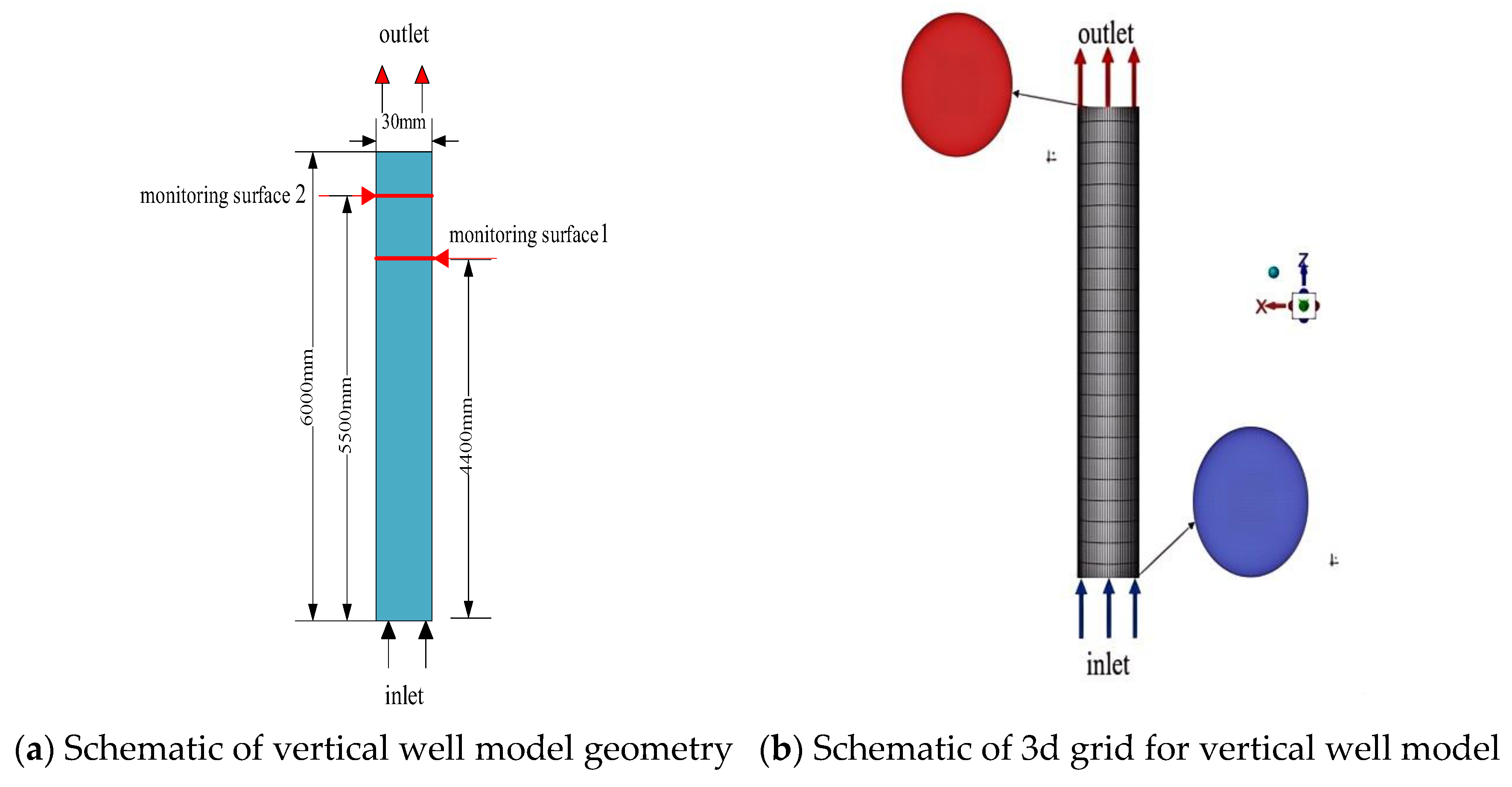
3.1. Geometric Model and Grid Generation

A vertical well model with a diameter of 30 mm was established. To ensure adequate flow of heavy oil–water two-phase fluid, the length of the model well was set to 20 times the well diameter (6000 mm), and flow parameter monitoring surfaces were established at 4500 mm and 5500 mm of the model. The geometric structure is shown in Figure 1a. The model was then discretized into a grid, and boundary layers were set near the wellbore wall, as shown in Figure 1b.

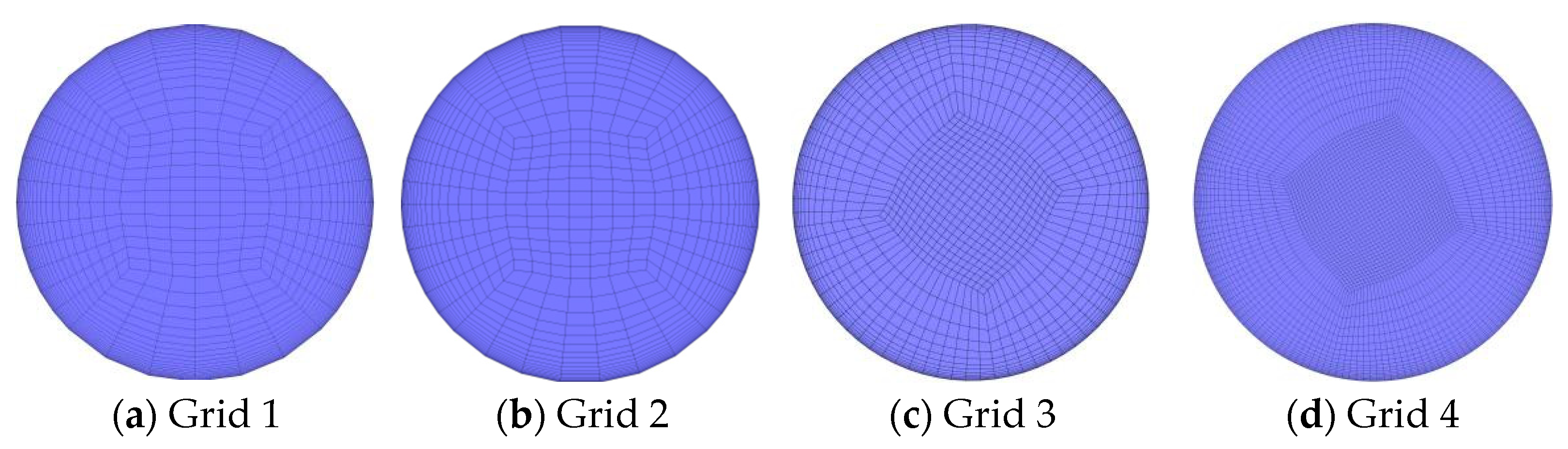
3.2. Boundary Conditions and Grid Independence Verification

The boundary conditions of the numerical model are presented in

Table 2. Boundary conditions.

	Content	Parameters
Inlet	Velocity inlet	0.8 m/s
Outlet	Pressure outlet	Standard atmospheric pressure
Wall boundary conditions	No-slip wall	Standard wall function

. The heavy oil and water are injected from the inlet shown in Figure 1a, and the effect of gravity is considered, with its direction along the negative z-axis as indicated in Figure 1b. The Coupled algorithm was employed for the resolution of the problem, with a convergence criterion of 10⁻⁶ scalar residuals for the energy equation and 10⁻³ for the remaining equations, and a time step of 0.001 s.

The number of grid cells is related to the accuracy of the calculation results. As the number of grid cells increases, the numerical error caused by grid discretization decreases, resulting in more accurate results. However, excessive grid cells can also increase the computational load. Therefore, before commencing the calculation, an analysis of grid independence must be performed to select an appropriate grid density, ensuring both computational efficiency and the accuracy of the results.

An O-type grid was adopted in this study and four different grid quantities were set by changing the radial grid density, as shown in Figure 2. The specific grid data are presented in

Table 3. Grid data.

Grid	Total Grid Count
1	220,518
2	326,118
3	507,285
4	1,027,431

.

To perform grid independence verification for the various grid quantities listed in Table 3, the average pressure difference between the two monitoring surfaces (shown in Figure 1a) during the time interval of 9–12 s was used as the verification basis. The experimental media parameters for the grid independence verification are presented in

Table 4. Media properties.

Medium	Density	Dynamic Viscosity (30 °C)	Oil–Water Interfacial Tension
Water	1.14 g/cm3	1.003 mPa·s	/
Oil	1.027 g/cm3	100 mPa·s	30 m N/m

.

As can be seen from Figure 3, after the grid quantity reaches 507,285, further increasing the number of grids does not significantly affect the calculated pressure difference between the two cross-sections. Therefore, considering both the accuracy of the simulation data and the efficiency of the simulation, a grid quantity of 507,285 was chosen for the calculations.

3.3. Model Validation

To guarantee the precision of the selected numerical computational model, the flow patterns of the 20 sets of numerical simulation experiments were contrasted with the 20 sets of physical experiments presented in the thesis. The physical parameters of oil and water utilized in this experiment are illustrated in

Table 5. Summary of parameters.

Temperature (°C)	Water Density (g/cm3)	Oil Density (g/cm3)	Water Viscosity (mPa·s)	Oil Viscosity (mPa·s)	Oil–Water Interfacial Tension (m N/m)
30	1.014	0.857	0.8	97.32	32.8

.

As evidenced by the data presented in

Table 6. Comparison between simulation results and experimental data.

No.	Mixing Flow Rate (m/s)	Water Content (%)	Flow Patterns		Consistency
			Experimental Data	Simulation Results
1	0.2	10	Bubble Flow	Bubble Flow	Yes
2	0.1	30	Slug Flow	Slug Flow	Yes
3	0.5	45	Slug Flow	Slug Flow	Yes
4	0.5	35	Slug Flow	Slug Flow	Yes
5	0.5	20	Bubble Flow	Bubble Flow	Yes
6	0.9	10	Bubble Flow	Bubble Flow	Yes
7	1	40	Slug Flow	Bubble Flow	No
8	1.2	15	Bubble Flow	Bubble Flow	Yes
9	1.4	95	Bubble Flow	Bubble Flow	Yes
10	1.8	10	Bubble Flow	Bubble Flow	Yes
11	0.5	55	Transitional Flow	Slug Flow	No
12	0.5	60	Slug Flow	Slug Flow	Yes
13	0.7	85	Bubble Flow	Bubble Flow	Yes
14	0.7	70	Slug Flow	Slug Flow	Yes
15	0.9	30	Bubble Flow	Bubble Flow	Yes
16	0.9	60	Slug Flow	Slug Flow	Yes
17	1.4	40	Slug Flow	Bubble Flow	No
18	1.4	70	Bubble Flow	Bubble Flow	Yes
19	1.8	30	Slug Flow	Slug Flow	Yes
20	1.8	70	Bubble Flow	Bubble Flow	Yes

, the level of concordance between the numerical modelling experiments and the outcomes of the physical experiments is 90%. While there are some discrepancies between the outcomes of Models 7, 11, and 17, this may be attributed to a number of factors, including the potential for observational errors, alterations in the physical and chemical characteristics of the experimental medium, and the influence of the experimental setting. Notwithstanding the aforementioned discrepancies, they remain within an acceptable range, thereby rendering the numerical modelling experimental calculations suitable for analysis.

4. Research on the Identification of Flow Patterns in Heavy Oil–Water Two-Phase Flow

The methods for identifying two-phase flow patterns are typically classified into two categories. The first is the direct determination of flow patterns based on the flow images of the two phases, including visual inspection and high-speed photography. The second category is the identification method based on the characteristics of changes in flow parameters, which involves collecting the time-varying signals of flow-related parameters (such as pressure, differential pressure, and liquid holdup) of the oil–water two-phase flow and obtaining the statistical characteristics of the signals (PDF) through harmonic analysis [24,25,26,27,28,29,30]. This article comprehensively adopts the above two methods to identify flow patterns.

Liquid holdup refers to the ratio of the area of the water phase A_w to the total area A on the monitoring surface during the flow of oil–water two-phase fluids. Therefore, the characteristics of liquid holdup changes can reflect certain properties of the flow patterns to a certain extent:

$$H_W={\displaystyle \frac{A_W}{A}}={\displaystyle \frac{A_W}{A_O+A_W}}$$

(9)

where A is the total area of the monitored surface, m²; A_w is the water phase area, m²; Ao is the oil phase area, m².

Therefore, the liquid holdup data of the flow patterns were recorded at the monitoring surface located at 5500 mm of the model (as shown in Figure 1a). Through the analysis of three types of information, including the liquid holdup curve, the probability density function (PDF) curve of liquid holdup, and the flow pattern contour maps of oil–water two-phase flow, six typical heavy oil–water two-phase flow patterns were identified: water-in-oil bubble flow (B W/O, as shown in Figure 4a), transitional flow (TF, as shown in Figure 4b), water-in-oil slug flow (S W/O, as shown in Figure 4c), oil-in-water bubble flow (B O/W, as shown in Figure 4d), oil-in-water very fine dispersed flow (VFD O/W, as shown in Figure 4e), and water-in-oil core-annular flow (Core-annular W/O, as shown in Figure 4f). In the flow pattern contour maps, the oil phase is represented by red, and the water phase is represented by blue.

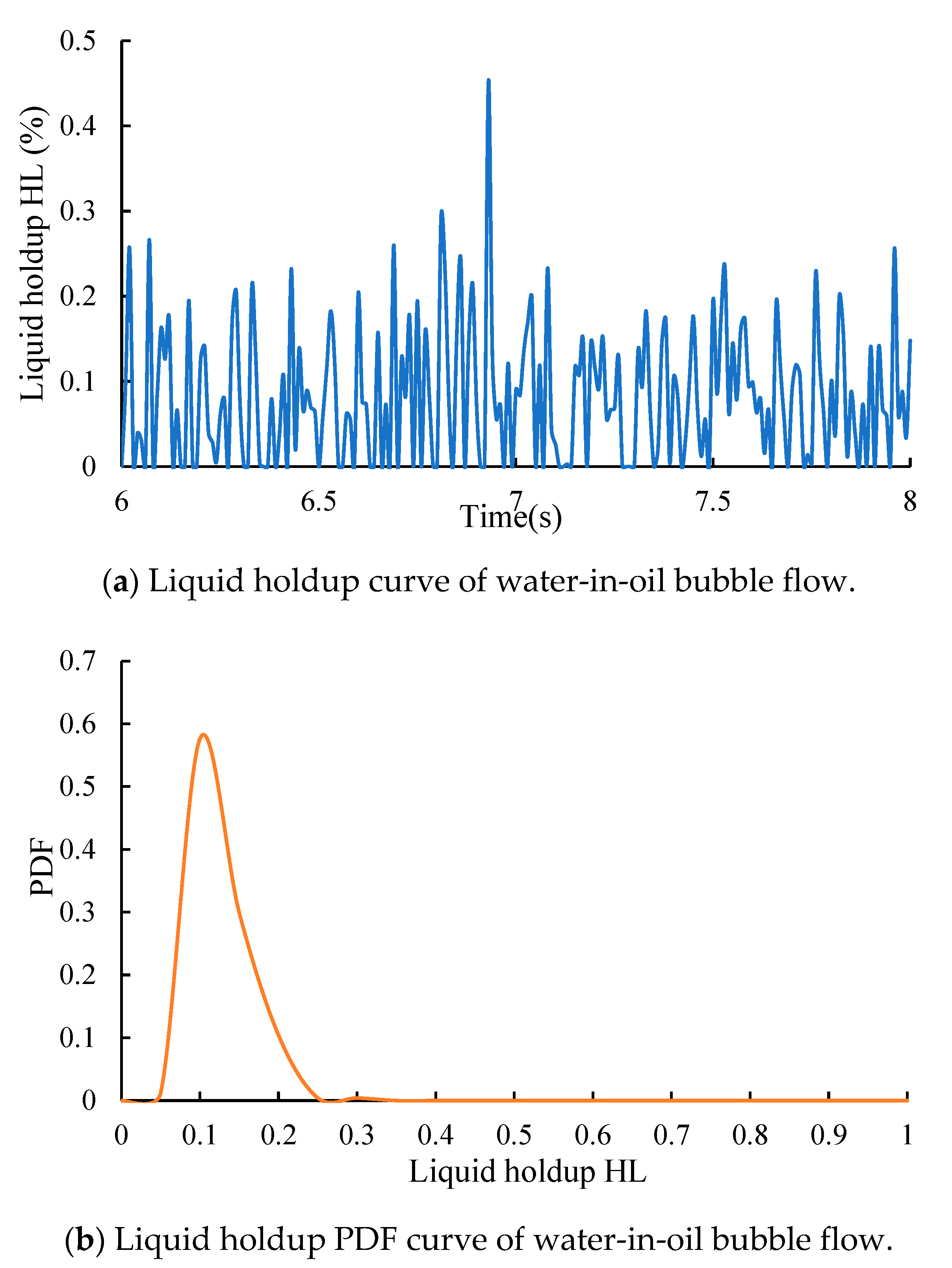
4.1. Water-in-Oil Bubble Flow (B W/O)

Water-in-oil bubble flow tends to occur when the inlet water cut is less than 30%. As shown in Figure 4a, in this flow pattern, the oil phase is the continuous phase, and the water phase is uniformly dispersed in the oil phase in the form of bubbles.

As can be seen from Figure 5, the liquid holdup curve of the water-in-oil bubble flow exhibits high-frequency oscillations, indicating that the bubbles passing through the monitoring surface are relatively dense within a unit time. The liquid holdup values generally oscillate within the range of 0 to 0.3, but occasionally, abnormally large values occur due to the aggregation of adjacent bubbles. The PDF curve of liquid holdup exhibits a unimodal shape, and the liquid holdup value at the peak is generally between 0 and 0.3.

In the field data verification, the actual flow pattern is unknown. During the flow pattern identification, a large fluctuation in the liquid holdup curve is observed, which may be related to the complex flow pattern change in heavy oil–water two-phase flow. In this study, the standard k-ω turbulence model was selected to deal with problems such as a low Reynolds number, significant interaction between fluid and sidewall, and a decrease in flow velocity. Therefore, the large fluctuation of liquid holdup may be caused by the characteristics of turbulence, the change in flow pattern, and the interaction between fluid and wellbore.

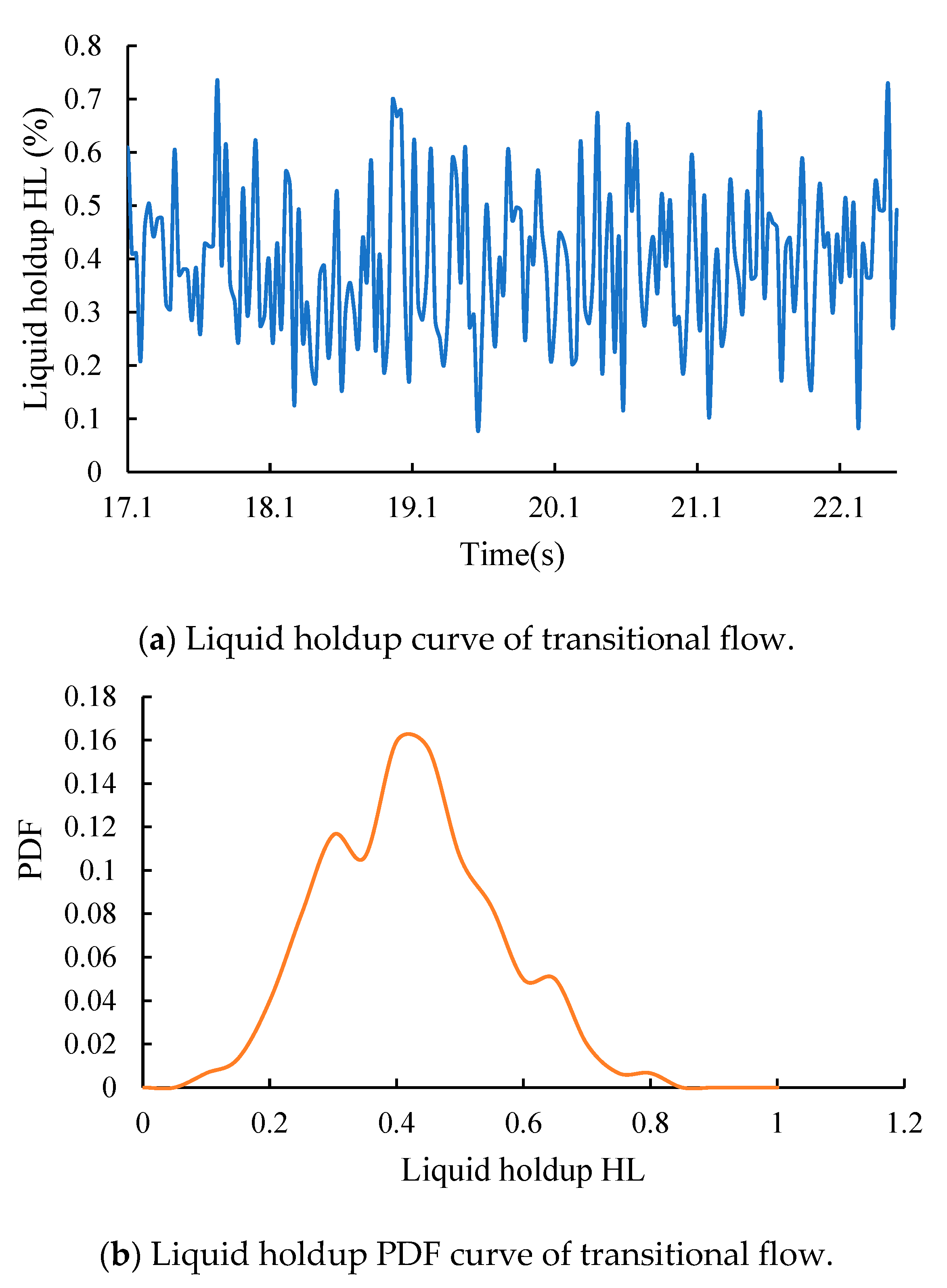
4.2. Transitional Flow (TF)

Transitional flow tends to occur when the inlet water content is between 20% and 60%. As shown in Figure 4b, neither the oil phase nor the water phase can form a stable continuous phase under these conditions.

As shown in Figure 6, the liquid holdup curve of the transition flow exhibits high-frequency and large-scale fluctuations, indicating that the flow pattern is unstable, resulting in irregular changes in the volume fractions of the water and oil phases. The fluctuation range of the liquid holdup value is between 0.2 and 0.8, and the PDF curve of liquid holdup exhibits multiple incomplete peak characteristics.

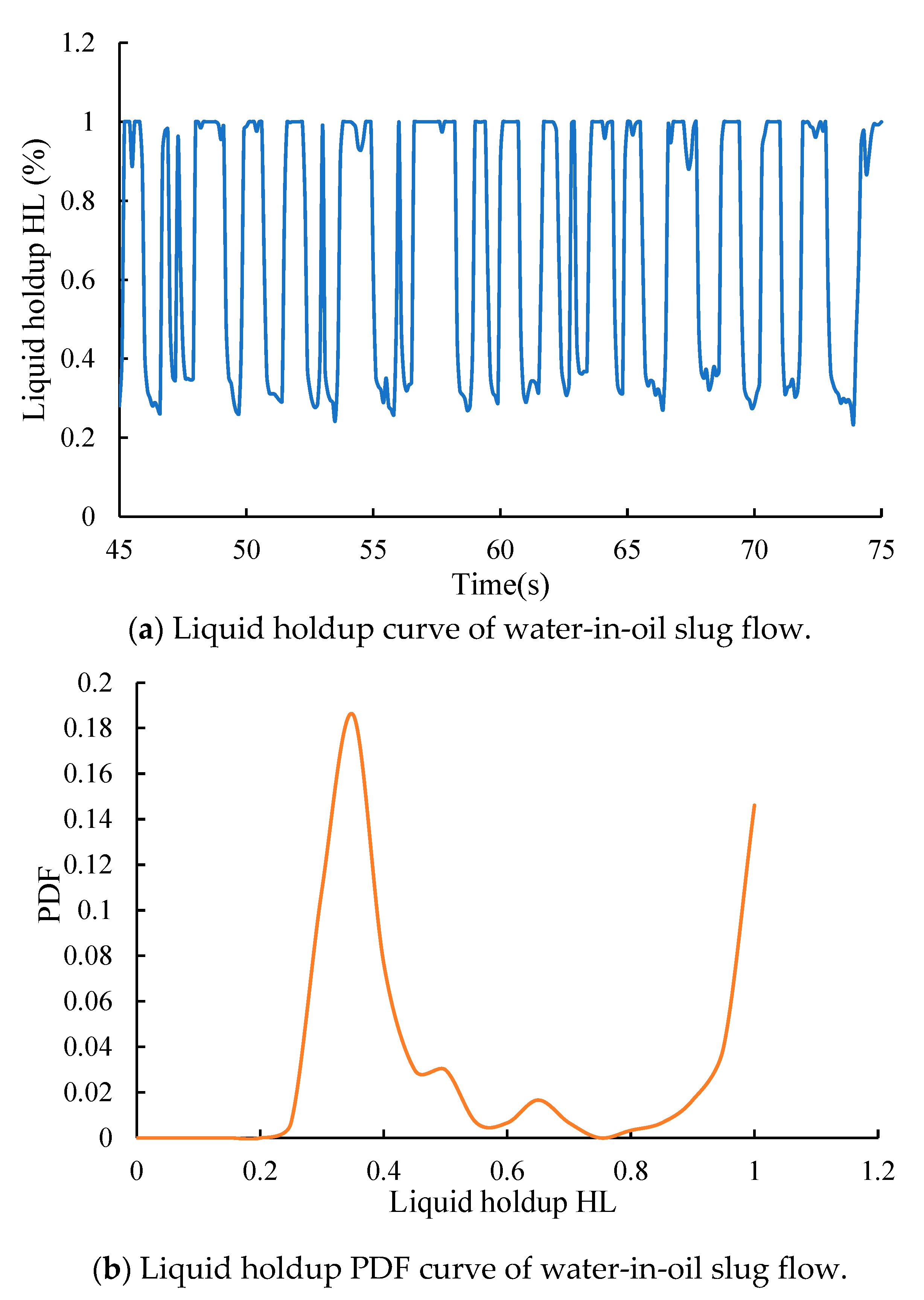
4.3. Water-in-Oil Slug Flow (S W/O)

Water-in-oil slug flow tends to occur when the inlet water cut is between 30% and 70%. As shown in Figure 4c, under this flow pattern, the oil phase is the continuous phase, while the water phase forms slugs of pipe diameter size.

As shown in Figure 7, the liquid holdup curve of the water-in-oil slug flow exhibited an overall low-frequency vibration phenomenon. This is because the water slug passing through the monitoring plane is relatively long within a unit of time. The liquid holdup curve displays a characteristic of gradual decline and steep rise. This is due to the relatively smooth head of the water slug, resulting in a gradual decrease in liquid holdup when the slug passes through the monitoring plane. After the water slug passes, the oil phase mixed with fine water bubbles begins to pass through the monitoring plane, causing the liquid holdup to sharply rise to its highest value. The presence of fine oil bubbles leads to uneven peaks in the curve. In addition, the PDF curve of liquid holdup exhibits a bimodal feature, with one peak at a low liquid holdup (0~0.4) and another peak at a high liquid holdup (close to 1).

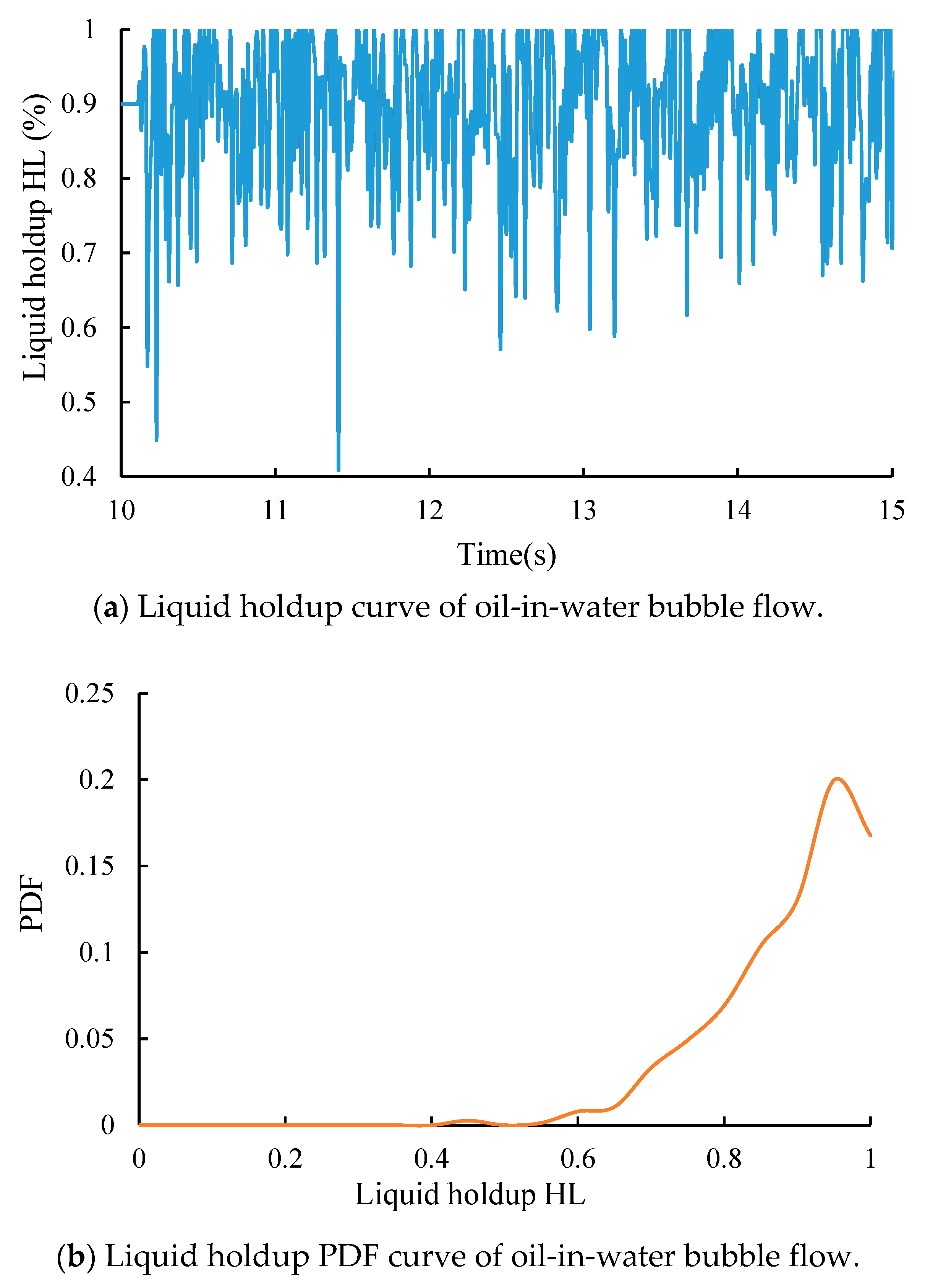
4.4. Oil-in-Water Bubble Flow (B O/W)

Oil-in-water bubble flow typically occurs when the heavy oil viscosity is between 100 and 2200 mPa·s and the inlet water cut is greater than 70%. As shown in Figure 4d, under this flow pattern, the water phase serves as the continuous phase, while the oil phase is dispersed in the water phase in the form of oil bubbles.

As seen in Figure 8, the liquid holdup curve of oil-in-water bubble flow exhibits high-frequency vibrations due to the influence of relatively dense small oil bubbles. The liquid holdup values generally oscillate within the range of 0.7 to 1, with occasional abnormally large values resulting from the aggregation of adjacent oil bubbles. Additionally, the randomness of oil bubble formation is quite strong, manifesting in a wide range of changes in liquid holdup values. The PDF curve of liquid holdup presents a unimodal shape, and the liquid holdup value at the peak is close to one.

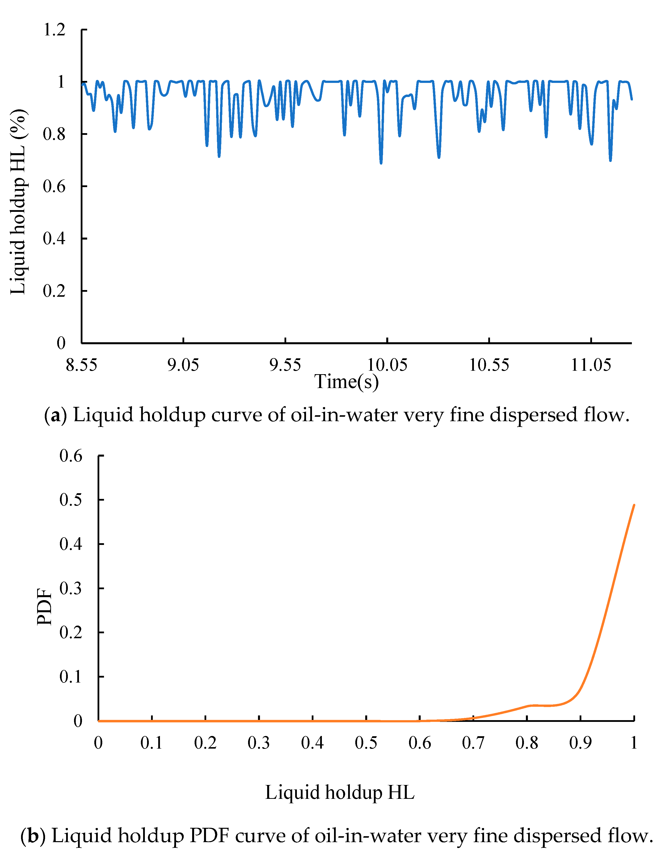
4.5. Oil-in-Water Very Fine Dispersed Flow (VFD O/W)

The oil-in-water very fine dispersed flow only occurs when the viscosity of heavy oil is 100 mPa·s and the inlet water cut is greater than or equal to 90%. As shown in Figure 4e, in this flow pattern, the water phase is the continuous phase, while the oil phase is dispersed in the water phase in the form of small and sparse oil bubbles.

According to Figure 9, the liquid holdup curve of the very fine dispersed oil-in-water bubble flow vibrates slightly at a low frequency, indicating that the water bubbles passing through the monitoring plane per unit time are small and few in number. The liquid holdup value generally vibrates between 0.8 and 1, and the PDF curve of the liquid holdup exhibits a single peak at a liquid holdup value of 1.

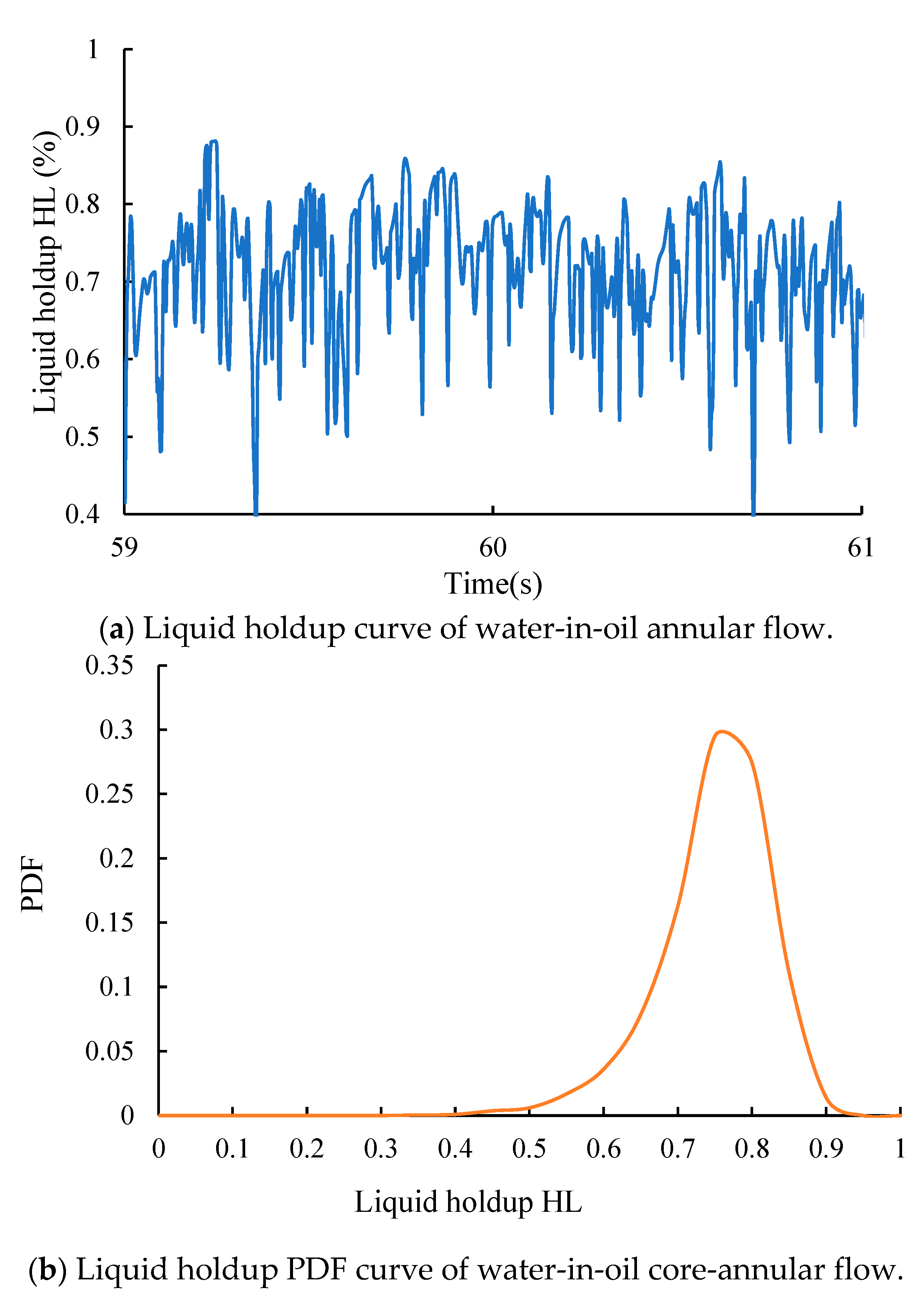
4.6. Water-in-Oil Core-Annular Flow (Core-Annular W/O)

Water-in-oil core-annular flow generally occurs when the heavy oil viscosity is greater than or equal to 600 mPa·s and the inlet water cut is greater than 70%. As shown in Figure 4f, under this flow pattern, both the oil and water phases are continuous, with the water phase being the core located in the middle of the pipeline, while the oil phase forms an outer ring surrounding the water phase.

As can be seen from Figure 10, the liquid holdup curve of oil-in-water core-annular flow exhibits high-frequency vibrations, oscillating around the average liquid holdup (0.7 in the Figure 10.). This is due to the interfacial fluctuation characteristics between the oil and water phases. The PDF curve of liquid holdup features a single peak, which is located at the average liquid holdup (0.7 in the Figure 10.).

5. Study on the Flow Patterns of Heavy Oil–Water Two-Phase Flow

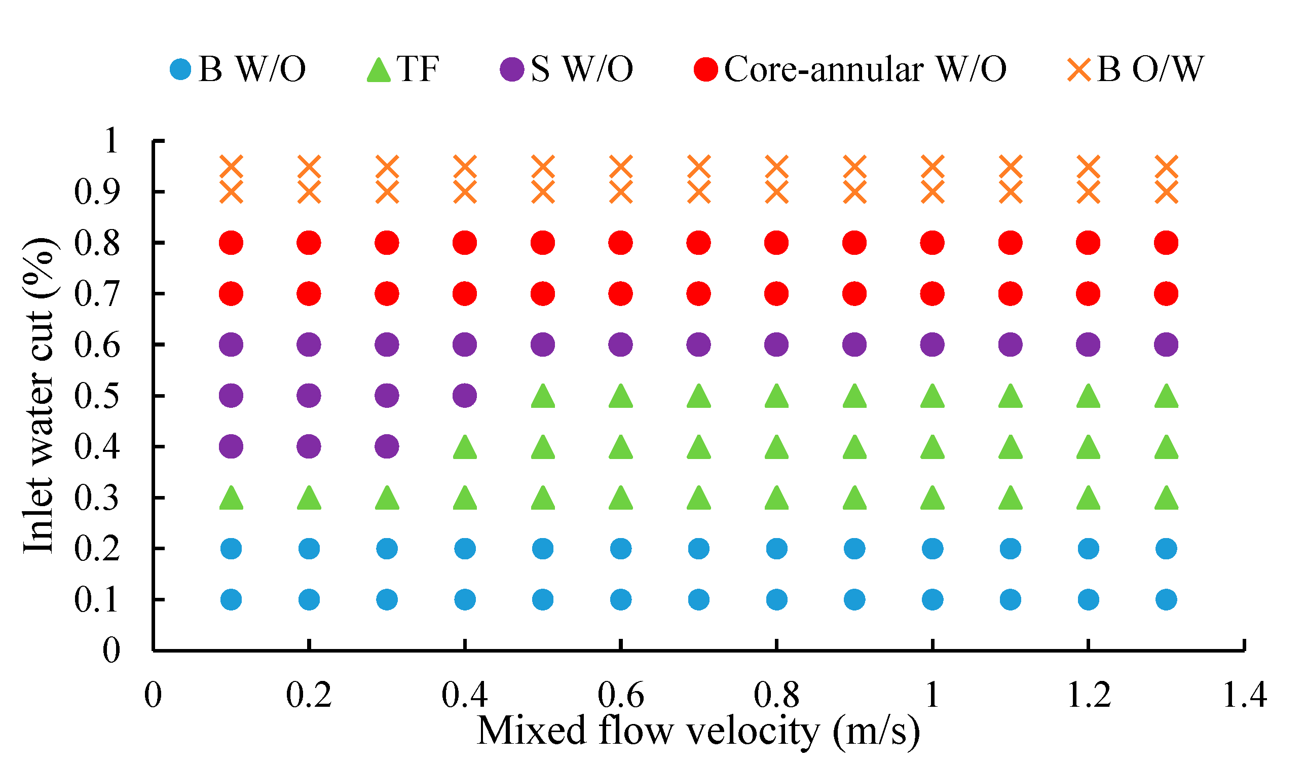
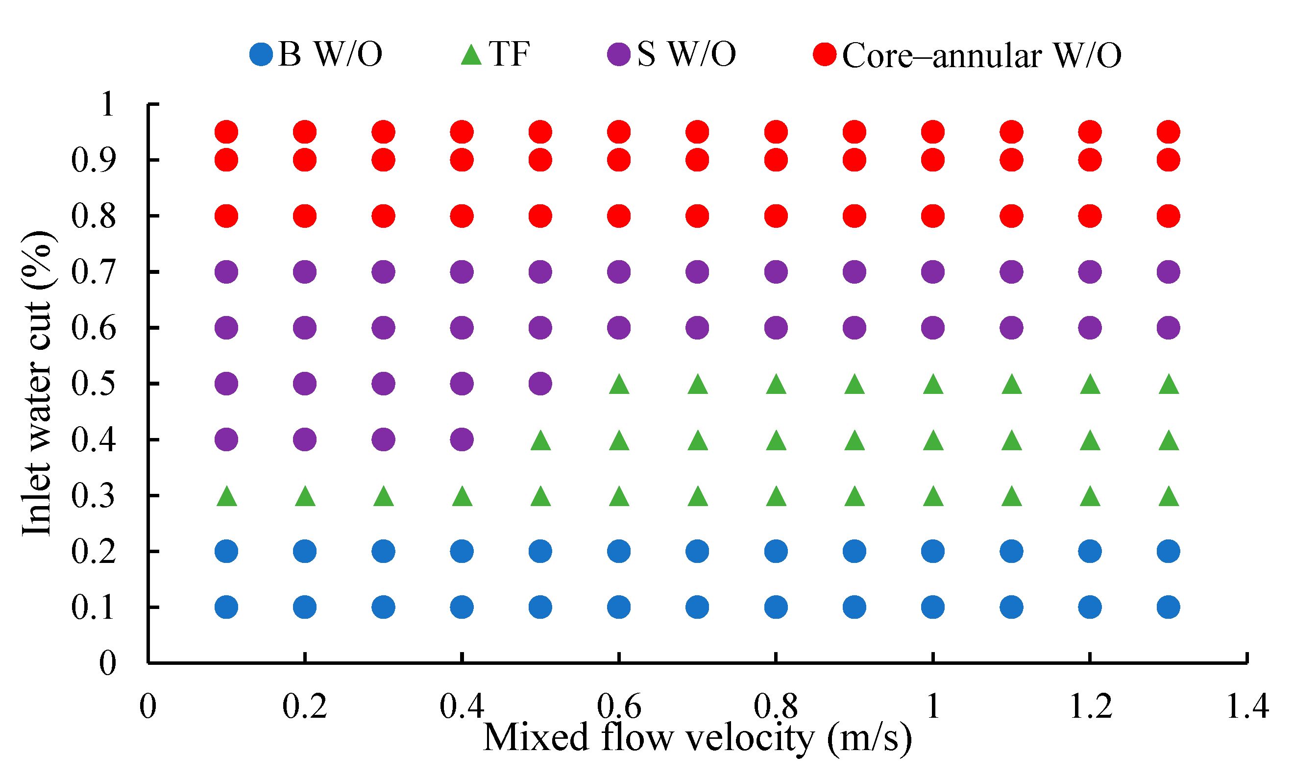
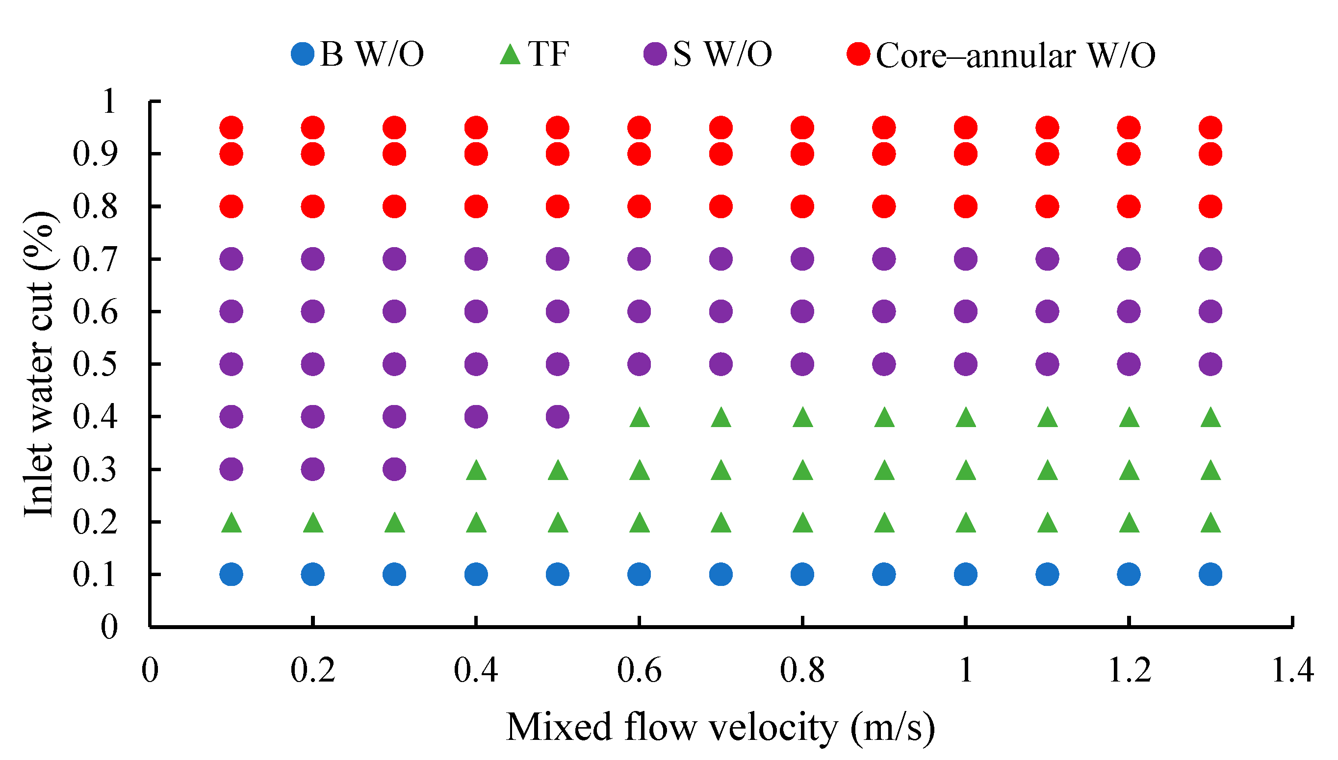
5.1. Development of Flow Pattern Maps

As seen in Figure 11, when the viscosity of heavy oil is 100 mPa·s, B W/O occurs at an inlet water cut of 0.1 to 0.3. As the inlet water cut rises to 0.3 to 0.5, TF appears. When the inlet water cut reaches 0.4 to 0.6, S W/O is observed. Between 0.7 and 0.8, the flow is primarily B O/W. At an inlet water cut greater than 0.9, VFD O/W emerges.

With the gradual increase in the mixed flow velocity, the regions of B W/O and VFD O/W expand, while the regions of S W/O, TF, and B O/W decrease. This is due to the increase in turbulent kinetic energy within the well as the mixed flow velocity rises, which disrupts some S O/W, resulting in the formation of TF. The TFs are disrupted into B W/O. The oil bubbles in the B O/W are dispersed into finer states, ultimately forming VFD O/W.

As seen in Figure 12, when the viscosity of heavy oil is 600 mPa·s, the flow is B W/O at an inlet water cut of 0.1 to 0.2. It transitions to TF at an inlet water cut of 0.3 to 0.5. S W/O is observed at an inlet water cut of 0.4 to 0.6. Core-annular W/O emerges at an inlet water cut of 0.7 to 0.8. And at an inlet water cut greater than 0.9, B O/W appears.

With the increase in mixed flow velocity, the region of S W/O decreases while the region of TF increases, indicating that an increase in mixed flow velocity disrupts some of the S W/O into TF. However, the other flow patterns are less affected by the change in mixed flow velocity under this viscosity.

Comparing the flow pattern map at 100 mPa·s (Figure 10), there are significant changes in flow patterns at 600 mPa·s. The B O/W at an inlet water cut of 0.7 to 0.8 disappears and transforms into Core-annular W/O. The VFD O/W transitions to B O/W. There are also notable changes in the regions of some flow patterns, with the region of S W/O relatively increasing and the regions of B W/O and TF relatively decreasing.

Figure 13 depicts the oil–water two-phase flow pattern map when the viscosity of heavy oil is 1100 mPa·s. At an inlet water cut of 0.1 to 0.2, the flow is B W/O. It transitions to TF at an inlet water cut of 0.3 to 0.5. At an inlet water cut of 0.4 to 0.7, S W/O is observed. Core-annular W/O emerges when the inlet water cut exceeds 0.8.

With the increase in mixed flow velocity, the region of S W/O decreases while the region of TF increases. There are still no significant changes in other flow patterns at this viscosity.

When compared to the flow pattern map at 600 mPa·s (Figure 12), the B O/W that was present at inlet water cuts greater than 0.9 transforms into Core-annular W/O. The regions of S W/O, Core-annular W/O, and TF increase, while the region of B W/O remains largely unchanged.

Figure 14 represents the oil–water two-phase flow pattern map for heavy oil with a viscosity of 2200 mPa·s. At an inlet water cut of 0.1 to 0.2, the flow is B W/O. TF emerges at an inlet water cut of 0.3 to 0.5. S W/O is observed at an inlet water cut of 0.4 to 0.7. Core-annular W/O appears when the inlet water cut exceeds 0.8.

With the increase in mixed flow velocity, the region of S W/O decreases while the region of TF increases. There are still no significant changes in other flow patterns at this viscosity.

Compared to the flow pattern map at 1100 mPa·s (Figure 13), the flow patterns remain the same. However, in the range of inlet water cut from 0.4 to 0.5 and mixed flow velocity from 0.1 to 0.5 m/s, some TF transitions into S W/O.

Figure 15 illustrates the oil–water two-phase flow pattern map for heavy oil with a viscosity of 5000 mPa·s. At an inlet water cut of 0.1, the flow is B W/O. TF emerges when the inlet water cut ranges from 0.2 to 0.4. The flow pattern transitions to S W/O between an inlet water cut of 0.3 and 0.7. Core-annular W/O appears when the inlet water cut exceeds 0.8.

With the increase in mixed flow velocity, the region of S W/O decreases while the region of TF increases. There are still no significant changes in other flow patterns at this viscosity.

Compared to the flow pattern map at 2200 mPa·s (Figure 14), we observe that as the viscosity of heavy oil increases to 5000 mPa·s, B W/O at an inlet water cut of 0.2 transitions to TF. Additionally, part of the TF at inlet water cuts of 0.3 to 0.5 transforms into S W/O.

In summary, as the viscosity of heavy oil increases from 100 mPa·s to 5000 mPa·s: ① Core-annular W/O emerges when the viscosity reaches 600 mPa·s, while B O/W and VFD B O/W completely disappear at a viscosity of 1100 mPa·s. This indicates that as the viscosity of heavy oil increases, the adhesion between the oil phase and the wellbore wall enhances, making it easier for the oil phase to become the continuous phase in contact with the wellbore wall. Water phase does not form a continuous phase when the viscosity exceeds 1100 mPa·s. ② At a constant viscosity, S W/O tends to occur in low-velocity regions, and the range of S W/O decreases with increasing flow velocity. This is because as the flow velocity increases, the turbulent kinetic energy also increases, making it difficult to form stable S W/O. However, as the viscosity of heavy oil increases, the region of S W/O increases significantly. This may be due to the buffering effect of viscous oil on turbulent kinetic energy. The higher the viscosity, the stronger the buffering effect, and the remaining turbulent kinetic energy is insufficient to disrupt S W/O. ③ After the viscosity of heavy oil increases, B W/O at an inlet water cut of 0.2 disappears and transforms into TF. This suggests that as the viscosity of the oil phase increases, the water phase is more likely to accumulate, leading to the early appearance of higher water cut flow patterns (TF).

5.2. Verification of Flow Pattern Maps

A certain heavy oil well W1 in an oilfield was selected as the experimental well, and CPS logging was performed on this well. As shown in

Table 7. CPS logging curve interpretation data table.

	Tube ID (mm)	76 mm
	Test Instrument Dia (mm)	38.0 mm
Explanation of test values	Pure oil: 30,159 CPS	Pure water: 11,636 CPS

, the closer the test value is to 11,636 CPS, the higher the water content in the well. Conversely, when the test value approaches 30,159 CPS, it indicates a higher oil content in the well.

The blending point of the W1 well is located at 6345 m. The production data above the blending point (6192 m) are shown in

Table 8. Production data above blending point of W1 well.

Parameter	Numerical Value
Production	97 t/d
Pipe ID	76 mm
Diluent density	910 kg/m3
Heavy oil density	1020 kg/m3
Water density	1140 kg/m3
Flow rate	39.64 m3/d
Viscosity of heavy oil after dilution	136 mPa·s
Flow velocity	0.25 m/s
Water cut	45%

, and the CPS data measured below the blending point are illustrated in Figure 16. The production data below the blending point (6362 m) are presented in

Table 9. Production data below blending point of W1 well.

Parameter	Numerical Value
Production	44 t/d
Pipe ID	62 mm
Heavy oil density	1020 kg/m3
Water density	1140 kg/m3
Undiluted flow rate	39.64 m3/d
Viscosity of undiluted heavy oil	632 mPa·s
Flow velocity	0.152 m/s
Water cut	78%

, and the spot-measured CPS data are shown in Figure 17.

As seen in Figure 16, during the continuous downward testing process, a large water slug appeared at a well depth of 2000 m, and a small water slug flow occurred at a depth of 6000 m. The reason for the slugging is that after blending with diluent, the viscosity of crude oil decreases, and the water slug segment is broken up. As the temperature gradually decreases, the viscosity of heavy oil increases, causing water-in-oil slug flow to reappear near the wellhead. The curve in Figure 17 represents the change in water cut at a depth of 6352 m over the measured time. As can be seen from the Fig., the curve exhibits high-frequency fluctuations with small amplitudes, and the water cut is relatively high, indicating a water-in-oil annular flow.

The above measured conclusions indicate that as the temperature gradually decreases above the blending point, S W/O occurs, while below the blending point, Core-annular W/O is present.

By incorporating the data from above the blending point in Table 6 of the W1 well into the map shown in Figure 18 and comparing it with the actual measured results, the map predicts the flow pattern above the blending point to be S W/O. Similarly, incorporating the data below the blending point of the W1 well into the map shown in Figure 19 and comparing it with the actual measured results, the map predicts the flow pattern below the blending point to be Core-annular W/O. This conclusion aligns with the actual test results, verifying the accuracy of the flow pattern map.

6. Conclusions

After conducting experimental research on the flow patterns of heavy oil–water two-phase flow in vertical wells, the following conclusions were drawn:

(1)

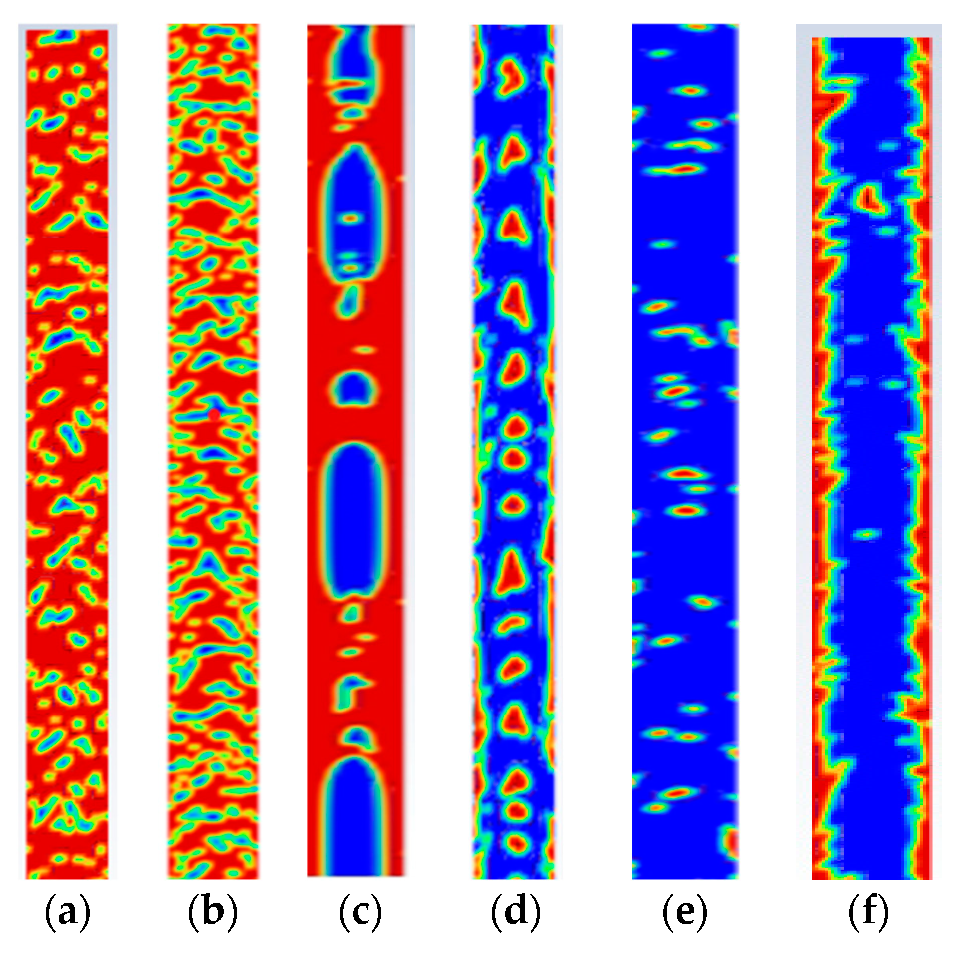
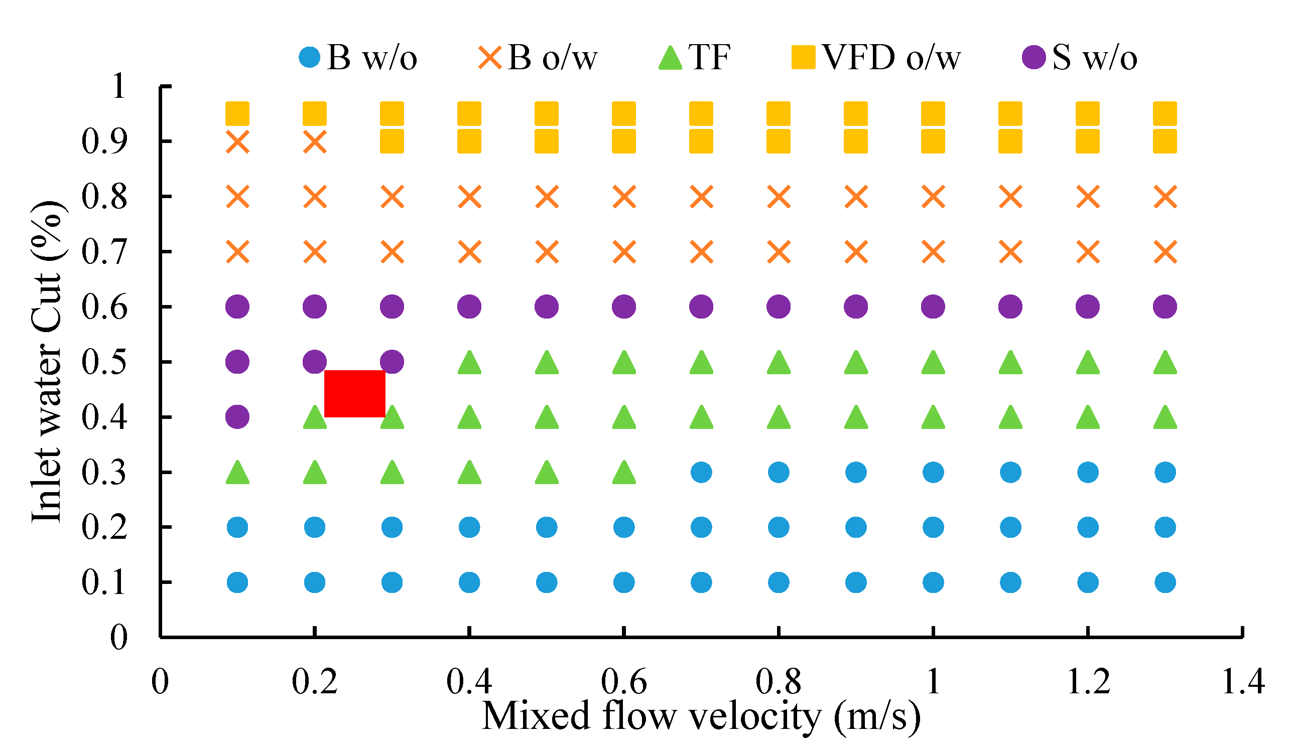
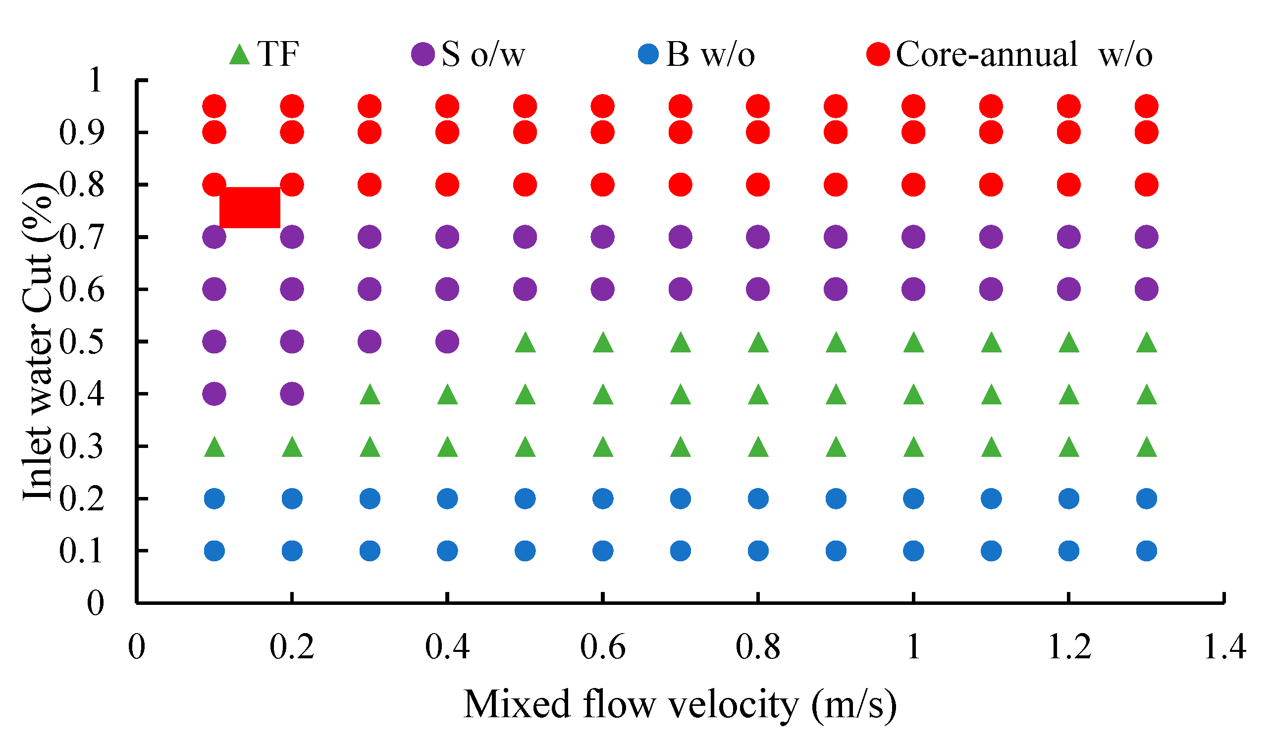
There are six typical flow patterns for heavy oil–water two-phase flow: water-in-oil bubble flow (B W/O), transitional flow (TF), water-in-oil slug flow (S W/O), oil-in-water bubble flow (B O/W), oil-in-water very fine dispersed flow (VFD O/W), and water-in-oil core-annular flow (Core-annular W/O).

(2)

When the viscosity of heavy oil reaches 600 mPa·s, Core-annular W/O appears. However, flow patterns with water as the continuous phase (B O/W and VFD O/W) completely disappear when the viscosity increases to 1100 mPa·s.

(3)

S W/O tends to occur in low-velocity regions. When the viscosity remains unchanged, the larger the flow velocity, the smaller the S W/O region; conversely, the higher the viscosity of heavy oil, the larger the area where S W/O appears.

(4)

As the viscosity of the oil phase increases, the water phase is more likely to aggregate, and B W/O is more prone to transition to TF.

(5)

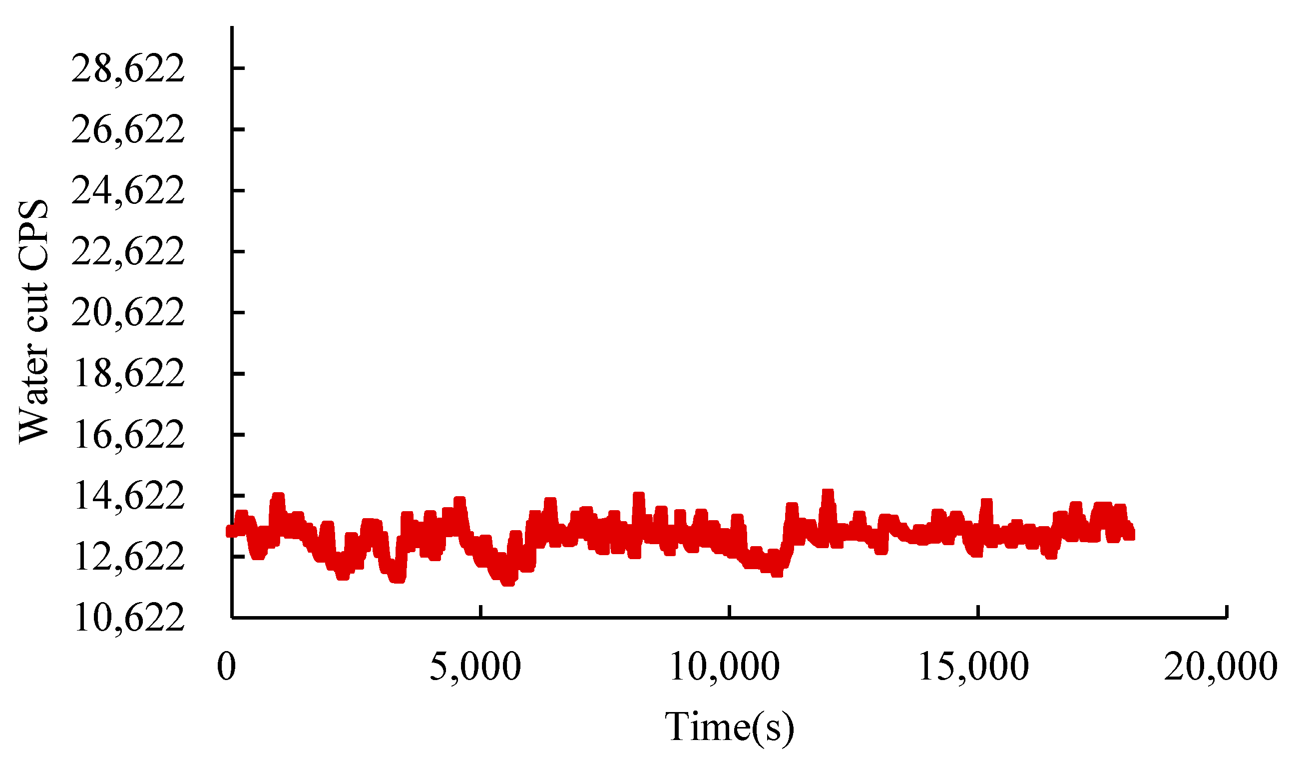
Based on the comparison and verification of the measured data from the W1 well with the heavy oil–water two-phase flow pattern map, the chart predicts that the flow pattern above the blending point of the well belongs to S W/O, and the flow pattern below the blending point belongs to Core-annular W/O, which is basically consistent with the actual measured flow pattern.

References

1. Liu, X.; Wu, T.; Ge, T.; Du, C.; Wang, D.; Geng, Z. In-situ Enhanced Oil Recovery Techniques for Heavy and Super-Heavy Oil. Contemp. Chem. Ind. 2023, 52. [Google Scholar] [CrossRef]
2. Hua, W.; Cai, L.; Xu, R.; Liu, T.; Yue, Y. Study on Flow Characteristics of Oil-Water Two-Phase Flow. Pet. Ind. Technol. Superv. 2022, 38, 28–31. [Google Scholar]
3. Charles, M.E.; Lilleleht, L.V. Correlation of pressure gradients for the stratified laminar-turbulent pipeline flow of two immiscible liquids. Can. J. Chem. Eng. 1966, 44, 47–49. [Google Scholar] [CrossRef]
4. Govier, G.W.; Sullivan, G.A.; Wood, R.K. The upward vertical flow of oil-water mixtures. Can. J. Chem. Eng. 1961, 39, 67–75. [Google Scholar] [CrossRef]
5. Hasan, A.R.; Kabir, C.S. A new model for two-phase oil/water flow: Production log interpretation and tubular calculations. SPE Prod. Eng. 1990, 5, 193–199. [Google Scholar] [CrossRef]
6. Zavareh, F.; Hill, A.D.; Podio, A.L. Flow regimes in vertical and inclined oil/water flow in pipes. In Proceedings of the SPE Annual Technical Conference and Exhibition, Houston, TX, USA, 2–5 October 1988; SPE: Kuala Lumpur, Malaysia, 1988. SPE-18215-MS. [Google Scholar]
7. Zhong, X.; Huang, Z.; Lv, P.; Xie, R.; Li, H. Study on Flow Pattern Identification of Oil-Water Two-Phase Flow in a 125 mm Vertical Circular Pipe. Acta Pet. Sin. 2001, 5, 89–94. [Google Scholar]
8. Jana, A.K.; Das, G.; Das, P.K. Flow regime identification of two-phase liquid–liquid upflow through vertical pipe. Chem. Eng. Sci. 2006, 61, 1500–1515. [Google Scholar] [CrossRef]
9. Mydlarz-Gabryk, K.; Pietrzak, M.; Troniewski, L. Study on oil–water two-phase upflow in vertical pipes. J. Pet. Sci. Eng. 2014, 117, 28–36. [Google Scholar] [CrossRef]
10. Hamidi, M.J.; Karimi, H.; Boostani, M. Flow Patterns and heat transfer of oil-water two-phase upward flow in vertical pipe. Int. J. Therm. Sci. 2018, 127, 173–180. [Google Scholar] [CrossRef]
11. Yang, Y.; Guo, J.; Ren, B.; Zhang, S.; Xiong, R.; Zhang, D.; Cao, C.; Liao, Z.; Zhang, S.; Fu, S.; et al. Oil-Water flow Patterns, holdups and frictional pressure gradients in a vertical pipe under high temperature/pressure conditions. Exp. Therm. Fluid Sci. 2019, 100, 271–291. [Google Scholar] [CrossRef]
12. Huang, L.; Wang, Y.; Cheng, X.; Wen, M.; Kang, X.; Lv, R.; Zhang, H.; He, J.; Yang, Y. Prediction Model of Water Holdup and Pressure Drop Based on the Flow Patterns of Heavy Oil-Water Two-Phase Flow in Vertical Pipelines. Sci. Technol. Eng. 2021, 21, 14908–14917. [Google Scholar]
13. Mazza, R.A.; Suguimoto, F.K. Experimental investigations of kerosene-water two-phase flow in vertical pipe. J. Pet. Sci. Eng. 2020, 184, 106580. [Google Scholar] [CrossRef]
14. Ganat, T.; Hrairi, M.; Gholami, R.; Abouargub, T.; Motaei, E. Experimental investigation of oil-water two-phase flow in horizontal, inclined, and vertical large-diameter pipes: Determination of flow Patterns, holdup, and pressure drop. SPE Prod. Oper. 2021, 36, 946–961. [Google Scholar] [CrossRef]
15. Farrar, B.; Bruun, H.H. A computer based hot-film technique used for flow measurements in a vertical kerosene-water pipe flow. Int. J. Multiph. Flow 1996, 22, 733–751. [Google Scholar] [CrossRef]
16. Descamps, M.; Oliemans, R.; Ooms, G.; Mudde, R.; Kusters, R. Influence of gas injection on phase inversion in an oil–water flow through a vertical tube. Int. J. Multiph. Flow 2006, 32, 311–322. [Google Scholar] [CrossRef]
17. Abduvayt, P.; Manabe, R.; Watanabe, T.; Arihara, N. Analysis of oil/water-flow tests in horizontal, hilly terrain, and vertical pipes. SPE Prod. Oper. 2006, 21, 123–133. [Google Scholar] [CrossRef]
18. Zhao, D.; Guo, L.; Hu, X.; Zhang, X.; Wang, X. Experimental study on local characteristics of oil–water dispersed flow in a vertical pipe. Int. J. Multiph. Flow 2006, 32, 1254–1268. [Google Scholar] [CrossRef]
19. Xu, J.; Li, D.; Guo, J.; Wu, Y. Investigations of phase inversion and frictional pressure gradients in upward and downward oil–water flow in vertical pipes. Int. J. Multiph. Flow 2010, 36, 930–939. [Google Scholar] [CrossRef]
20. Du, M.; Jin, N.D.; Gao, Z.K.; Wang, Z.Y.; Zhai, L.S. Flow Pattern and water holdup measurements of vertical upward oil–water two-phase flow in small diameter pipes. Int. J. Multiph. Flow 2012, 41, 91–105. [Google Scholar] [CrossRef]
21. Zhang, J.; Xu, J.; Wu, Y.; Li, D.; Li, H. Experimental validation of the calculation of phase holdup for an oil–water two-phase vertical flow based on the measurement of pressure drops. Flow Meas. Instrum. 2013, 31, 96–101. [Google Scholar] [CrossRef]
22. Han, Y.; Jin, N.; Ren, Y.; He, Y. Measurement of pressure drop and water holdup in vertical upward oil-in-water emulsions. IEEE Sens. J. 2017, 18, 1703–1713. [Google Scholar] [CrossRef]
23. Hirt, C.W.; Nichols, B.D. Volume of fluid (VOF) method for the dynamics of Free Boundaries. J. Comput. Phys. 1981, 39, 201–225. [Google Scholar] [CrossRef]
24. Zhang, L. Experimental Study and Transient Numerical Calculation of Gas-Liquid Two-Phase Flow in Pipelines. Ph.D. Thesis, Wuhan University, Wuhan, China, 2020. [Google Scholar]
25. Ma, Y. Research on Flow Pattern Identification Method of Oil-Water Two-Phase Capacitance Tomography. Master’s Thesis, Northeast Petroleum University, Daqing, China, 2020. [Google Scholar]
26. Feng, N. Numerical Simulation of Gas-Liquid Two-Phase Stirred Flow in a Vertical Rising Pipe. Master’s Thesis, Xi’an Shiyou University, Xi’an, China, 2019. [Google Scholar]
27. Ye, W. Reconstruction of a Multi-functional Experimental Device for Downward Flow of Gas-Liquid Two-Phase in Wellhead Injection. Master’s Thesis, Southwest Petroleum University, Daqing, China, 2019. [Google Scholar]
28. Chen, L.; Yin, J.; Sun, Z.; Yao, F.; Zhou, T. Flow Pattern Identification of Bluff Body Flow around Gas-Liquid Two-Phase Flow Based on EEMD-Hilbert Spectrum. Chin. J. Sci. Instrum. 2017, 38, 2536–2546. [Google Scholar]
29. Zhang, X.; Li, L.; Hu, H. Flow Pattern Identification of Gas-Solid Two-Phase Flow Based on EEMD and Fractal Box Dimension. J. Northwest Univ. (Nat. Sci. Ed.) 2016, 46, 178–183. [Google Scholar]
30. Yu, H. Ultrasonic Echo Attenuation Characteristics of Gas-Liquid Two-Phase Flow Pipe Wall and Its Application. Master’s Thesis, China University of Petroleum (East China), Qingdao, China, 2015. [Google Scholar]
Figure 1. Schematic diagram of the vertical well model.
Processes 12 02404 g001
Figure 2. Schematic diagram of radial grid distribution.
Processes 12 02404 g002
Figure 3. Pressure difference between two monitoring surfaces for different grids.
Processes 12 02404 g003
Figure 4. Contour maps of six typical heavy oil–water two-phase flow patterns. (a) B W/O; (b) TF; (c) S W/O; (d) B O/W; (e) VFD O/W; (f) Core-annular W/O.
Processes 12 02404 g004
Figure 5. Liquid holdup and liquid holdup PDF curve of water-in-oil bubble flow.
Processes 12 02404 g005
Figure 6. Liquid holdup and liquid holdup PDF curve of transitional flow.
Processes 12 02404 g006
Figure 7. Liquid holdup and liquid holdup PDF curve of water-in-oil slug flow.
Processes 12 02404 g007
Figure 8. Liquid holdup and liquid holdup PDF curve of oil-in-water bubble flow.
Processes 12 02404 g008
Figure 9. Liquid holdup and liquid holdup PDF curve of oil-in-water very fine dispersed flow.
Processes 12 02404 g009
Figure 10. Liquid holdup and liquid holdup PDF curve of water-in-oil core-annular flow.
Processes 12 02404 g010
Figure 11. Oil–water two-phase flow pattern map for heavy oil viscosity of 100 mPa·s.
Processes 12 02404 g011
Figure 12. Oil–water two-phase flow pattern map for heavy oil viscosity of 600 mPa·s.
Processes 12 02404 g012
Figure 13. Oil–water two-phase flow pattern map for heavy oil viscosity of 1100 mPa·s.
Processes 12 02404 g013
Figure 14. Oil–water two-phase flow pattern map for heavy oil viscosity of 2200 mPa·s.
Processes 12 02404 g014
Figure 15. Oil–water two-phase flow pattern map for heavy oil viscosity of 5000 mPa·s.
Processes 12 02404 g015
Figure 16. Measured cps data above blending point of W1 well.
Processes 12 02404 g016
Figure 17. Measured CPS data below blending point of W1 well.
Processes 12 02404 g017
Figure 18. Comparison flow pattern map above the blending point.
Processes 12 02404 g018
Figure 19. Comparison flow pattern map below the blending point.
Processes 12 02404 g019