Modeling and Optimization of the Inland Container Transportation Problem Considering Multi-Size Containers, Fuel Consumption, and Carbon Emissions

Abstract

This paper investigates the inland container transportation problem with a focus on multi-size containers, fuel consumption, and carbon emissions. To reflect a more realistic situation, the depot’s initial inventory of empty containers is also taken into consideration. To linearly model the constraints imposed by the multiple container sizes and the limited number of empty containers, a novel graphical representation is presented for the problem. Based on the graphical representation, a mixed-integer programming model is presented to minimize the total transportation cost, which includes fixed, fuel, and carbon emission costs. To efficiently solve the model, a tailored branch-and-price algorithm is designed, which is enhanced by improvement schemes including a heuristic label-setting algorithm, decremental state-space relaxation, and the introduction of a high-quality upper bound. Results from a series of computational experiments on randomly generated instances demonstrate that (1) the proposed branch-and-price algorithm demonstrates a superior performance compared to the tabu search algorithm and the genetic algorithm; (2) each additional empty container in the depot reduces the total transportation cost by less than 1%, with a diminishing marginal effect; (3) the rational configuration of different types of trucks improves scheduling flexibility and reduces fuel and carbon emission costs as well as the overall transportation cost; and (4) extending customer time windows also contributes to lower the total transportation cost. These findings not only deepen the theoretical understanding of inland container transportation optimization but also provide valuable insights for logistics companies and policymakers to improve efficiency and implement more sustainable operational practices. Additionally, our research paves the way for future investigations into the integration of dynamic factors and emerging technologies in this field.

1. Introduction

With rising global awareness of the pressing need to combat climate change, the focus on reducing fuel consumption and carbon emissions has intensified across numerous sectors. The transportation industry, a major contributor to greenhouse gas emissions, has particularly come under the spotlight due to its significant environmental impact and high fuel usage. It is estimated that the transportation sector accounts for approximately 21% of global CO₂ emissions, with road freight transport accounting for nearly three-quarters of transport emissions [1]. In pursuit of environmental protection, governments are striving for a low-carbon economy through the implementation of rigorous emission reduction and fuel efficiency regulations [2]. Consequently, the transportation industry is confronted with increasing pressure to align with these sustainability goals. In the realm of intermodal container transportation, the inland container transportation involves the short-distance movement of outbound and inbound containers between terminals, depots, and customers. This process addresses the initial and final segments of a container’s journey within the intermodal transportation chain. Undoubtedly, inland container transportation also stands out as a substantial contributor to carbon emissions due to the fuel-intensive nature of truck-based transport [3]. To meet sustainability objectives and reduce environmental impact, it is essential to optimize inland container transportation with an emphasis on reducing both fuel consumption and carbon emissions.

The inland container transportation problem (ICT) addresses the efficient routing of trucks to handle the collection and distribution of full and empty containers within a local area. A major challenge in addressing the ICT lies in the management of multiple container sizes. With the expansion of global trade, the variety of container sizes used in shipping has grown. Among the various container sizes, the 20 ft and 40 ft containers are the most prevalent [4]. The variety in container sizes complicates the ICT, as the presence of different container sizes makes the combinations for container assignments and routing options more flexible yet also more complex. Additionally, empty containers are often in limited supply at depots, posing another significant challenge. Specifically, maintaining a large inventory of empty containers at the depot tends to be financially burdensome due to the considerable costs associated with their purchase, storage, and maintenance. For example, new 20 ft storage containers generally cost between USD 3000 and USD 6000, while 40 ft storage containers can range from USD 6000 to USD 12,000 [5]. For truck firms with fluctuating container needs, it may be economically impractical to keep a large stock of empty containers. Failing to account for these limitations in route planning can lead to inefficient or unfeasible routing plans, impacting overall operational effectiveness. In this context, efficiently addressing the ICT by managing limited empty containers, accommodating different container sizes, and reducing carbon emissions and fuel consumption is crucial for enhancing the efficiency and sustainability of the container transportation industry.

In the existing literature, some studies have explored the ICT with multi-size containers [6,7,8,9,10,11,12,13]. The difficulty in modeling the ICT with multi-size containers is ensuring that the total number of containers loaded onto a truck stays within its capacity. Current methodologies, including state-transition schemes, decoupling-and-coupling mechanisms, and request-and-transport layer techniques, are notably intricate and somewhat difficult to follow. In contrast, we propose a more straightforward modeling technique that can reduce these complexities. Furthermore, the literature reveals a substantial gap in research on the ICT with restricted empty container availability [14,15,16,17]. This gap is highlighted by the fact that many existing studies in this domain simplify the problem by considering only a single container size, which fails to reflect the diverse realities of situations involving multiple container sizes. Another gap is found in the way constraints on the depot’s inventory of empty containers are modeled. Most studies use non-linear constraints, which can lead to inefficiencies. Instead, our proposed modeling approach addresses this by linearly modeling these constraints. Besides, existing studies predominantly emphasize economic efficiency, such as minimizing distance or total travel cost, with limited attention to environmental concerns like fuel consumption and carbon emissions. This study explicitly integrates both economic and environmental objectives, offering a balanced optimization that accounts for cost-effectiveness and sustainability. Therefore, this paper not only addresses the ICT with limited empty container availability and multiple container sizes but also incorporates environmental concerns, such as fuel consumption and carbon emissions. The principal contributions of this paper are summarized below:

(1)

We propose a simple but effective graph modeling approach to represent the problem on a directed network. The graph model not only simplifies the handling of capacity-related constraints arising from multiple container sizes but also enables the linear representation of the constraints posed by the limited empty containers, thereby facilitating the development of a mathematical formulation for the problem.

(2)

A tailored branch-and-price algorithm is presented for the problem. For efficient resolution of the pricing subproblems, we suggest a hybrid algorithm which integrates an exact label-setting algorithm, improved through the decremental state-space relaxation, with its heuristic counterpart. Besides, an upper bounding scheme is proposed to prune nodes.

(3)

Numerical tests are performed to verify the effectiveness of the proposed algorithm. Furthermore, a sensitivity analysis is performed to examine the effects of various factors, providing valuable insights for managerial decision making.

The structure and logical flow of this paper are presented in Figure 1.

2. Literature Review

The ICT has attracted considerable academic attention over the past two decades, resulting in numerous significant findings.

Table 1. Existing studies on ICTs.

Paper	Feature				Objective	Model	Solution Method
	Multi-Size	Empty Con.	Heter.	Carbon			Solver	Exact	Heuristic
[6]	✓		✓		Minimal Cost	Non-linear			✓
[7]	✓				Minimal Cost	Linear			✓
[8]	✓				Minimal Distance	Linear			✓
[9]	✓		✓		Minimal Cost	Linear		✓
[10]	✓				Minimal Time	Non-linear			✓
[11]	✓				Minimal Distance/Time	Linear	✓
[12]	✓				Minimal Time	Linear	✓
[13]	✓		✓		Minimal Cost	Linear		✓	✓
[14]		✓			Minimal Time	Non-linear			✓
[15]		✓			Minimal Time/Truck	Non-linear			✓
[16]		✓		✓	Minimal Cost	Non-linear			✓
[17]		✓			Minimal Cost	Linear		✓
[18]				✓	Minimal Emissions	Linear			✓
[19]				✓	Minimal Emissions	Non-linear			✓
[20]				✓	Minimal Time	Linear			✓
[21]				✓	Minimal Fuel/Emissions	Non-linear			✓
Our study	✓	✓	✓	✓	Minimal Fuel/Emissions	Linear		✓	✓

“Multi-size”: multi-size containers; “Empty con.”: limited empty containers; “Heter.”: heterogeneous trucks; “Carbon”: carbon emissions.

provides a comparative summary of some papers, highlighting the problem aspects considered and the solution methods applied. Existing studies closely related to our research scope can be broadly classified into three categories: the ICT involving multi-size containers, ICT with limited empty containers, and ICT considering carbon emissions.

2.1. ICT with Multi-Size Containers

A majority of existing studies on the ICT mainly center on situations with one-size containers. Readers can refer to Chen et al. [22] for an extensive survey of relevant research. The insights and methodologies in this domain lay the foundation for more complicated variants involving multi-size containers. When it comes to the ICT with multi-size containers, Chung et al. [6] propose an insertion-based heuristic to explore an ICT that incorporates a heterogeneous truck fleet and various container sizes. In a related study, Vidović et al. [7] examine a similar issue and concentrate on optimizing the pairing of pickup and delivery requests to reduce total travel distance. Bruglieri et al. [8] extend the research of Vidović et al. [7] by adapting the problem to multi-period scenarios. Bustos-Coral and Costa [9] introduce a comprehensive modeling framework for the ICT that accommodates containers of varying sizes and cargo types, along with heterogeneous trucks. This method utilizes state-transition logic to address constraints related to the compatibility between trucks and containers, as well as the arrangement of loads. But, these works have limitations, particularly in their failure to account for the provision and repositioning of empty containers. As a result, the problem is essentially simplified to the vehicle routing problem with pickup and delivery.

Recognizing these gaps, some researchers have integrated the provision and repositioning of empty containers into their models. A significant contribution in this stream is by Zhang et al. [10]. They propose a state-transition-based model which can not be directly solved by commercial solvers, highlighting the complexity of modeling this problem. In response to this challenge, scholars have devoted considerable effort to developing models for the ICT with multi-size containers. Funke and Kopfer [11] offer a three-part modeling approach for this problem, which includes assigning containers, building routes, and integrating these components. Alternatively, Moghaddam et al. [12] present a generalized model for the ICT with multi-size containers using a two-layered graph structure to effectively manage timing and capacity constraints. Both models are evaluated through simulation-based experiments via MILP solvers, and no tailored algorithms are developed. In a subsequent study, Chen et al. [13] mainly focus on proposing a tailored MILP model with much fewer variables. They also introduce a heuristic algorithm to handle large-scale problems. Despite these advancements, the complexity of these models can make them challenging to follow. In contrast, our work proposes a more straightforward yet effective method for modeling the ICT with multi-size containers.

2.2. Ict with Limited Empty Containers

The high costs associated with purchasing and maintaining empty containers undoubtedly limit their availability at depots. To better reflect real-world situations, it is crucial to account for these limitations in ICT models. Nevertheless, research on this topic is still in its infancy. Zhang et al. [14] are pioneers in considering the constraints posed by limited empty containers. The problem is represented on a directed graph and treated as a variant of the multiple traveling salesman problem. A non-linear mathematical model is built and resolved using a reactive tabu search algorithm. Subsequently, Zhang et al. [15] further refine the model by linearizing the non-linear constraints associated with the limited availability of empty containers and developing a large neighborhood search algorithm for satisfactory solutions. Recently, Yu et al. [16] tackle a comprehensive ICT that integrates truck operation modes, limited empty containers, and multiple depots. They formulate this problem as an MILP model based on the DAOV graph, which is inspired by Zhang et al. [15]. Consequently, their model also incorporates non-linear constraints to reflect the depot’s restricted supply of empty containers. To handle this, they also resort to linearization techniques to convert the mathematical model into a linear form. And, given the complexity of this problem, an improved genetic algorithm is designed to achieve high-quality solutions. Additionally, Fazi et al. [17] propose a linear model aimed at the efficient re-use of empty containers through synchronization; however, this approach adds complexity to the model by including trips as variable indices. A common limitation of these studies is their focus on a single container size, whereas our research addresses the challenges posed by multiple container sizes, which aligns more closely with general situations.

2.3. Ict Considering Fuel Consumption and Carbon Emissions

The integration of fuel consumption and carbon emissions into the ICT has received attention in recent years. Zhang et al. [18] are among the first to address the ICT with a focus on a low-carbon objective. Based on the determined-activities-on-vertex graph, they develop an MILP model that minimizes total carbon emissions instead of traditional metrics like travel time. Subsequently, Konstantzos et al. [19] introduced a model to analyze greenhouse gas (GHG) emissions from terminal and container operations, providing a comprehensive assessment and strategies for mitigation. Building on the foundation laid by Konstantzos et al. [19], Shiri and Huynh [20] investigate the operational impact of various chassis supply models on transportation operations and carbon emissions. They introduce an innovative scheduling approach that treats tractors, containers, and chassis as distinct entities. Using a reactive tabu search algorithm, they demonstrate that a co-op pool, terminal pool, and rental pool with chassis yards inside terminals effectively reduce operational duration, minimize empty movements, and lower emissions. Following these efforts, He et al. [21] investigate the ICT with a separation mode to reduce fuel costs and carbon emissions. A mixed-integer programming model is introduced and effectively solved via an enhanced ant colony algorithm. Most recently, Yu et al. [16] enrich this field by integrating environmental considerations into a comprehensive ICT model. They concentrate on optimizing trucking operations and empty container relocations to minimize both fuel consumption and carbon emissions. The study demonstrates that strategic management can lead to substantial cost savings and emission reductions.

In summary, relatively extensive research has separately addressed multi-size containers, limited empty containers, fuel consumption, and carbon emissions, but the integration of all these aspects into a single model remains largely unexplored. Our work distinguishes itself by simultaneously considering these critical aspects and developing a straightforward yet effective model that linearly represents the constraints posed by multi-size containers and limited empty containers. Besides, most prior studies have concentrated on metaheuristic algorithms which lack optimality guarantees and often degrade in performance as problem size increases. In contrast, we propose a model-based branch-and-price algorithm capable of delivering optimal or near-optimal solutions to this complex problem.

3. Problem Description and Models

This section presents a detailed description of the problem and provides its graphical and mathematical models.

3.1. Problem Description

A truck firm provides container transportation services within an import-dominant region. The firm has a depot for stacking empty containers and parking trucks. There are two common sizes of containers: 20 ft (one 20 ft container = 1 TEU) and 40 ft containers. Due to physical space limitations and cost considerations, the depot maintains a limited inventory of empty containers in each size. There are two types of trucks: one with a capacity of 1 TEU, capable of carrying at most one 20 ft container, and another with a capacity of 2 TEU, capable of carrying at most two 20 ft containers or one 40 ft container.

Trucks depart from the depot to fulfill container transportation requests and have the flexibility to return to the depot at any time to store or retrieve empty containers. As a result, the inventory of empty containers of each size at the depot fluctuates dynamically as trucks carry out their transportation tasks. Upon completing these tasks, trucks must make their way back to the depot. Trucks are required to complete these requests within specified time windows set by the terminal and customers. Besides, the truck’s maximum allowable working time is restricted by the duration of the planning horizon. The optimization goal of this problem is to select the optimal truck transportation routes to minimize the total cost of completing all container transportation requests while ensuring the depot never experiences a stockout of empty containers.

Container transportation requests can be divided into two main categories according to the direction of flow: inbound containers and outbound containers. Each category can be further subdivided based on load status: full containers and empty containers. Therefore, container transportation requests include four types: outbound full (OF) containers, outbound empty (OE) containers, inbound full (IF) containers, and inbound empty (IE) containers. In ports where imports are dominant, the truck firm mainly handles the first three types of container transportation requests:

(1)

OF container transportation request. A truck transports an empty container to the shipper (origin). The container, once filled with goods, is then delivered by the truck to the terminal (destination) for export purposes.

(2)

OE container transportation request. Due to trade imbalances between regions, a certain quantity of empty containers needs to be transported to the terminal (destination) for export. It is worth mentioning that an OE request is not tied to a specific origin, as the empty container can be sourced from either the depot or a consignee;

(3)

IF container transportation request. A truck picks up a full container from the terminal (origin) and transports it to the designated consignee (destination). Once the container is emptied, the truck has several options: it can return the empty container to the depot, deliver it to another export customer for repacking, or transport it back to the terminal as an outbound empty (OE) container.

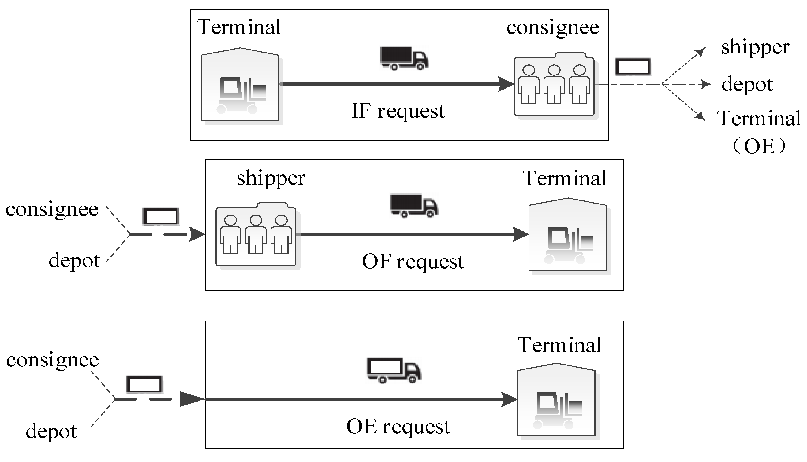
Considering the two different sizes of 20 ft and 40 ft containers, container trucks ultimately need to handle six different types of container transportation requests, i.e., $I{F}_{20}$, $I{F}_{40}$, $O{F}_{20}$, $O{F}_{40}$, $O{E}_{20}$, and $O{E}_{40}$. To illustrate container transportation requests, Figure 2 offers a schematic representation of three types of requests for 20 ft containers. This figure shows the requirement (release) of an empty container for each type of request, along with the potential source (destination) of the empty container. For example, an IF request will release an empty container after unpacking, and the emptied container may be transferred to a shipper, the depot, or the terminal. Therefore, determining the appropriate source (destination) for empty containers involved in IF, OF, and OE requests is a crucial element of the optimization process. In addition, when a truck with a capacity of 2 TEU fulfills a request concerning 20 ft containers, it might not move directly from its origin to its destination. Instead, it may take a detour to serve other requests related to 20 ft containers. The complexity of coordinating these movements further imposes considerable difficulties on the optimization process.

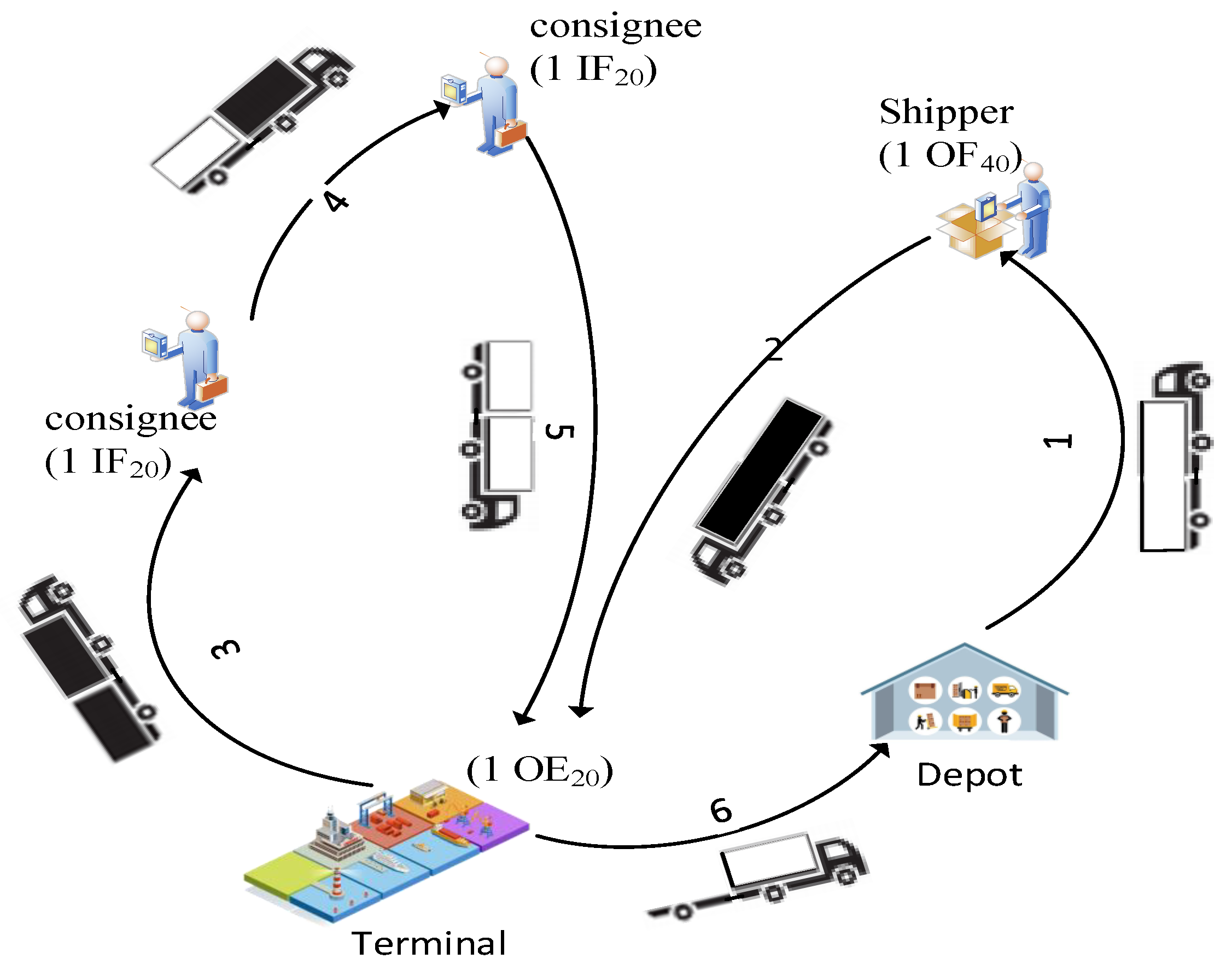
In order to gain a clearer insight into the problem discussed in this paper, Figure 3 provides a simplified case, which includes one terminal, one depot, one truck with a capacity of 2 TEU, and one 40 ft empty container at the depot. The firm needs to complete the following tasks: one $O{F}_{40}$ request (one customer needs to export one 40 ft full container), two $I{F}_{20}$ requests (each one needs to import one 20 ft full container), and one $O{E}_{20}$ request (one 20 ft empty container needs to be delivered to the terminal). Figure 3 illustrates a feasible truck route, with the numbers on the arrows indicating the sequence of the truck’s visits. Specifically, the truck starts by retrieving a 40 ft empty container from the depot and then travels to the shipper’s premises. Once the container is filled with goods, the truck proceeds to deliver it to the terminal ($O{F}_{40}$ request completed). Subsequently, the truck retrieves two inbound full containers and heads to the first consignee. After unpacking the goods for the first consignee (one $I{F}_{20}$ request completed), the truck proceeds to the second consignee with the left inbound full container and one container that was just emptied. After unpacking the goods for the second consignee (another $I{F}_{20}$ request completed), the truck transports the two empty 20 ft containers to the terminal. Here, one of the empty containers is offloaded as an outbound empty container ($O{E}_{20}$ request completed). Finally, the truck drags the remaining 20 ft empty container back to the depot.

3.2. Graphic Representation

Formulating a mathematical model for this problem, grounded in its original physical network, is particularly complex and challenging. An alternative way is to first represent the problem using a graph and then construct the mathematical model based on this graphical representation. As mentioned in the literature review, various graph modeling techniques are available, but they can be somewhat hard to follow. This paper introduces a more effective graph model with a simpler structure. The basic idea is as follows. Each request is associated with either an origin or a destination location, as shown in Figure 2. And, visiting any location involves picking up or delivering an empty or full container; otherwise, it is unproductive and can be avoided. Therefore, we can represent each container transportation request by nodes corresponding to the origin and/or destination. Accordingly, the changes in the number of empty and full containers on a truck can be determined when visiting these nodes. Undoubtedly, a visit to a specific node is allowed if the total number of empty and full containers the truck carries does not exceed its capacity. And, given the limited supply of empty containers at the depot, the depot will not run out of empty containers as long as the empty containers released by IF requests and returned to the depot are either kept in the depot or retrieved after their arrival at the depot. Based on this, we represent the problem on an innovative directed graph $G=(N,A)$, where N is the node set and A the arc set. The definitions of nodes are as follows.

3.2.1. Source and Sink Nodes

A source node is defined to represent the trucks’ departure from the depot, and a sink node is introduced to signify their eventual return to the depot.

3.2.2. Nodes for Container Transportation Requests

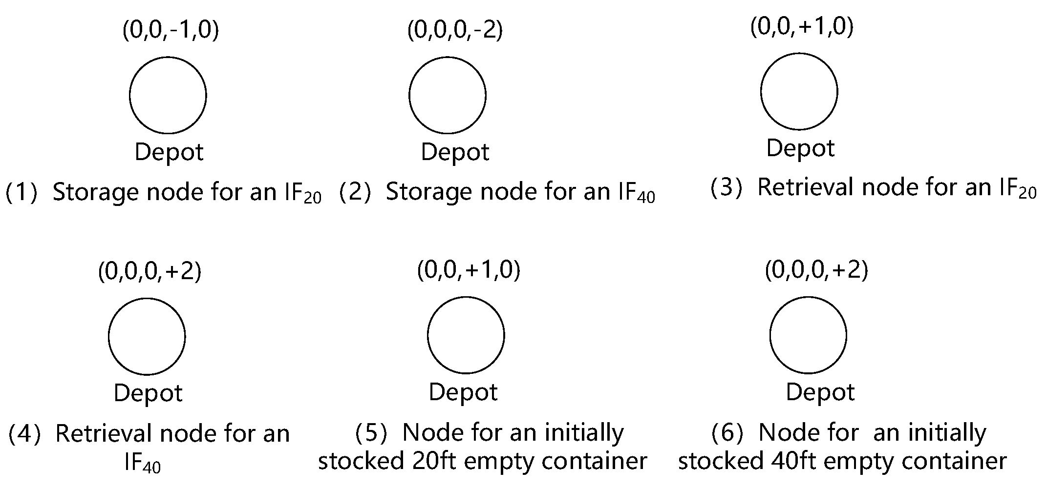
As illustrated in Figure 4, each $I{F}_{20},I{F}_{40},O{F}_{20}$, and $O{F}_{40}$ request is represented by two nodes, while each $O{E}_{20}$ and $O{E}_{40}$ request is symbolized by a single node. Each node is associated with either an origin or a destination location, as labeled in the figure. Additionally, the numbers in parentheses show the changes in the number of different-sized empty and full containers carried by a truck when it visits the corresponding node. These four numbers represent changes in the quantities (measured in TEUs) of 20 ft full containers, 40 ft full containers, 20 ft empty containers, and 40 ft empty containers, respectively. In the figure, +1 (−1) denotes an increase (decrease) in one 20 ft container for the truck, and +2 (−2) denotes an increase (decrease) in one 40 ft container for the truck.

Taking $I{F}_{20}$ as an example, as shown in Figure 4(1), the first node represents the pickup of an inbound full container from the terminal. Visiting this node increases the number of 20 ft full containers by one for the truck, and thus the changes for different-sized empty and full containers are labeled as (+1,0,0,0). The second node signifies the delivery of the previously picked-up full container to the consignee, unpacking goods, and then transporting away the emptied container. Visiting this node, the truck first decreases the quantity of 20 ft full containers by one and then increases the quantity of 20 ft empty containers by one. Thus, the changes for different-sized empty and full containers are recorded as (−1,0,+1,0). Similar deductions can be applied to determine the changes in empty and full containers associated with visiting other container transportation request nodes.

3.2.3. Node Representing Storage and Retrieval of an Empty Container from the Depot

Trucks have the option to return to the depot whenever necessary to either retrieve or offload empty containers. This paper introduces nodes to represent the storage and provision of empty containers at the depot.

(1) Node representing storage of an empty container to the depot.

After completing an $I{F}_{20}$ or $I{F}_{40}$ request, an empty container is released. This emptied container can either be stored at the depot, transferred to a shipper for packaging, or carried to the terminal as an OE container. The latter two scenarios are realized by visiting corresponding nodes defined for IF and OE requests, as illustrated in Section 3.2.2. For the first scenario, we additionally introduce a node to represent the storage of the empty container released by an $I{F}_{20}$ or $I{F}_{40}$ request to the depot. It is evident that when a truck visits such storage nodes associated with $I{F}_{20}$ and $I{F}_{40}$ requests, the resulting changes in the quantities of empty and full containers it carries are (−1,0,0,0) and (−2,0,0,0), respectively, as shown in Figure 5(1,2).

(2) Node representing retrieval of an empty container from the depot.

If a container truck retrieves empty containers from the depot, those containers may come from two possible sources: (i) the empty containers previously released by the IF request and stored in the depot or (ii) empty containers from the initial inventory at the depot.

For the first case, an additional node is introduced for each $I{F}_{20}$ and $I{F}_{40}$ request to represent the retrieval of the emptied containers which have already been returned and stored at the depot. The changes in the number of empty and full containers carried by the truck upon visiting these retrieval nodes are (+1,0,0,0) and (+2,0,0,0), as shown in Figure 5(3,4). Since the empty containers released by IF requests must be already stored in the depot before they can be retrieved, there exist temporal constraints between the storage nodes and their corresponding retrieval nodes introduced for IF requests. This further complicates the problem.

For the latter case, a node is similarly introduced for each initially inventoried 20 ft or 40 ft empty container to represent the retrieval of the corresponding container. When a truck visits such a node, the increments in the number of empty and full containers are (+1,0,0,0) for a 20 ft empty container and (+2,0,0,0) for a 40 ft empty container, as shown in Figure 5(5,6).

Therefore, the problem is formulated as a directed graph. And, a feasible truck route is depicted as a path in graph G that starts at the source node, passes through various intermediate nodes, and concludes at the sink node, adhering to the relevant constraints. A complete schedule is formed by multiple routes that collectively cover all request nodes. The objective is to identify a set of such routes that minimize the total transportation cost.

3.3. Mathematical Formulation

We introduce a mathematical model in this section, which is formulated from the graphical representation discussed previously. Given the depot’s limited initial inventory of empty containers, it is evident that the depot will never experience a stockout of empty containers if, and only if, the emptied container released from an IF request is retrieved after it has been transported and stored at the depot. Therefore, the restrictions posed by limited empty containers can be perfectly addressed by implementing temporal constraints between the storage nodes and the corresponding retrieval nodes introduced for IF requests, as previously mentioned. The capacity limit, measured in TEUs, can also be respected by tracking the total number of empty and full containers on a truck as it visits each node. On this basis, a mathematical formulation can be easily proposed for the problem. All parameters and variables referenced in this section are detailed in

Table 2. Parameters and variables.

Parameter	Description
N	Set of all nodes
K	Set of all trucks
S	Source node
$\mathcal{F}$	Sink node
$N^{\left(1\right)}$	Set of first nodes used to represent IF20, IF40, OF20, and OF40 requests
$N^{\left(2\right)}$	Set of second nodes used to represent IF20, IF40, OF20, and OF40 requests
$\tilde{\vartheta }\left(i\right)$	The corresponding second node for node $i\in N^{\left(1\right)}$
$N^{\left(o\right)}$	Set of nodes used to represent OE20 and OE40 requests
D	Set of nodes representing storage of empty containers released by IF requests to the depot
P	Set of nodes representing retrieval of empty containers released by IF requests and returned back to the depot
$P^S$	Set of nodes representing retrieval of empty containers initially stationed at the depot
${\alpha }_i$	Change in the number of 20 ft full containers when visiting node i, ${\alpha }_i\in \{-1,0,+1\}$
${\beta }_i$	Change in the number of 40 ft full containers when visiting node i, ${\beta }_i\in \{-2,0,+2\}$
${\gamma }_i$	Change in the number of 20 ft empty containers when visiting node i, ${\gamma }_i\in \{-1,0,+1\}$
${\delta }_i$	Change in the number of 40 ft empty containers when visiting node i, ${\delta }_i\in \{-2,0,+2\}$
$g_i$	Change in the payload of a truck when it visits node i, which can be determined based on associated handling operations and the weight of the empty container and its contents
$G^k$	Unladen weight of truck k, i.e., the total weight of the tractor and the trailer for truck k
$\xi$	Coefficient of the engine module
$\lambda$	Coefficient of the weight module
$\theta$	Coefficient of the speed module
$[a_i,b_i]$	Time window of node i
$T_i$	Time consumed by loading and unloading operations associated with node i
$d_{ij}$	Distance from node i to node j
v	The average travel speed of trucks
$T_{ij}$	Traveling time from node i to node j, which can be computed by $d_{ij}$/v
$\varphi$	Grams of CO2 emitted per liter of fuel
$Q_k$	Capacity of truck k (measured in TEUs), $Q_k\in \{1,2\}, k\in K$
$C_{fix}^k$	The fixed cost of truck k
$P_t$	Set of pairwise storage node $i\in D$ and the corresponding retrieval node $j\in P$ introduced for IF requests for which a temporal constraint exists
$C_{tax}$	The cost tax per unit of carbon emissions
$P_{fuel}$	The price of fuel
H	The planning horizon
M	A sufficiently large positive number
Variable	Description
$F_i^{1,k}$	The quantity of 20 ft full containers on truck k upon visiting node i
$F_i^{2,k}$	The quantity of 40 ft full containers on truck k upon visiting node i
$E_i^{1,k}$	The quantity of 20 ft empty containers on truck k upon visiting node i
$E_i^{2,k}$	The quantity of 40 ft empty containers on truck k upon visiting node i
$x_{ij}^k$	One if truck k travels through arc(i, j), zero otherwise
$y_i^k$	The time when truck k arrives at node i
$z_{ij}^k$	The payload weight of truck k on arc(i, j), i.e., the weight of full or empty containers carried by truck k

. The considered objectives are as follows.

(1) The fixed costs of trucks: The fixed costs are trucks’ one-time start-up costs, including truck depreciation, driver salaries, maintenance expenses, and other related costs. These fixed costs are incurred by those dispatched trucks, except idle ones. Notably, these costs are independent of the mileage traveled. The fixed costs $C_1$ can be expressed as Equation (1).

$$C_1=C_{fix}\sum _{j\in N}\sum _{k\in K}{x}_{Sj}^k$$

(1)

(2) The fuel and carbon emission costs: Carbon emissions during truck driving are primarily determined by fuel consumption, which is influenced by factors including the type of truck, driving speed, the weight of the truck and its cargo, and the length of the journey. To compute fuel consumption, we utilize the Comprehensive Modal Emission Model proposed by Barth et al. [23] and Barth and Boriboonsomsin [24]. Specifically, the fuel consumption for truck k traveling from node i to node j, i.e., along arc $(i,j)$, can be estimated by the formula $f_{ij}^k=\left[{\displaystyle \frac{\xi }{v}}+\lambda \left(G^k+z_{ij}^k\right)+\theta v^2\right]d_{ij}$, where $\xi$, $\lambda$, and $\theta$ are coefficients corresponding to the engine, weight, and speed modules, respectively. Here, $G^k$ represents the unladen weight of truck k, $z_{ij}^k$ is the payload weight of truck k, $d_{ij}$ is the distance of arc $(i,j)$, and v is the average speed of the truck. Let $P_{\mathrm{fuel}}$ denote the price of fuel and $x_{ij}^k$ be a 0–1 variable that takes the value 1 if truck k traverses arc $(i,j)$ and 0 otherwise. The total fuel cost, $C_2$, can then be expressed as Equation (2).

$$C_2=P_{fuel}\sum _{k\in K}\sum _{i\in N}\sum _{j\in N}{f}_{ij}^k{x}_{ij}^k$$

(2)

Let $\varphi$ be the grams of CO₂ emitted per liter of fuel consumed; the amount of CO₂ emissions resulting from the fuel consumption for truck k on the route from node i to node j can be calculated using the equation $O_{ij}^k=\varphi f_{ij}^k$. To quantify carbon emissions costs, this paper adopts a carbon tax mechanism. Assuming a carbon tax rate of $C_{tax}$, the carbon emissions cost $C_3$ can be expressed as Equation (3).

$$C_3=C_{tax}\sum _{k\in K}\sum _{i\in N}\sum _{j\in N}{O}_{ij}^k{x}_{ij}^k$$

(3)

Based on the previously mentioned costs, along with the parameters and variables, the problem can be mathematically formulated as follows:

$$min{C}_{fix}\sum _{j\in N}\sum _{k\in K}{x}_{Sj}^k+(P_{fuel}+C_{tax}\varphi )\sum _{k\in K}\sum _{i\in N}\sum _{j\in N}[\xi /v+\lambda (G^k+z_{ij}^k)+\theta v^2]d_{ij}{x}_{ij}^k$$

(4)

$$\mathrm{s}.\mathrm{t}.\sum _{k\in K}\sum _{j\in N}{x}_{ij}^k=1,\forall i\in N^{\left(1\right)}\cup N^{\left(2\right)}\cup N^{\left(O\right)}$$

(5)

$$\sum _{k\in K}\sum _{j\in N}{x}_{ij}^k\le 1,\forall i\in D\cup P\cup P^S$$

(6)

$$\sum _{j\in N}{x}_{Sj}^k\le 1,\forall k\in K$$

(7)

$$\sum _{j\in N}{x}_{ji}^k-\sum _{j\in N}{x}_{ij}^k=0,\forall i\in N\setminus \{S\cup \mathcal{F}\},k\in K$$

(8)

$$a_i\sum _{j\in N}{x}_{ij}^k\le y_i^k\le b_i\sum _{j\in N}{x}_{ij}^k,\forall i\in N,k\in K$$

(9)

$$y_i^k+T_i+T_{ij}\le y_j^k+(1-x_{ij}^k)M,\forall i,j\in N,k\in K$$

(10)

$$y_i^k+T_i+T_{i\tilde{\vartheta }\left(i\right)}\le y_{\tilde{\vartheta }\left(i\right)}^k+(1-\sum _{j\in N}{x}_{ij}^k)M,\forall i\in N^{\left(1\right)},k\in K$$

(11)

$$y_{\mathcal{F}}^k\le H,\forall k\in K$$

(12)

$$\sum _{k\in K}{y}_i^k-M\sum _{k\in K}{x}_{ij}^k\le \sum _{k\in K}{y}_j^k-M\sum _{k\in K}\sum _{h\in N}{x}_{jh}^k,\forall (i,j)\in P_t$$

(13)

$$F_i^{1,k}+{\alpha }_j\le F_j^{1,k}+(1-x_{ij}^k)M,\forall i\in N\setminus \mathcal{F},j\in N\setminus S,k\in K$$

(14)

$$F_i^{1,k}+{\alpha }_j\ge F_j^{1,k}-(1-x_{ij}^k)M,\forall i\in N\setminus \mathcal{F},j\in N\setminus S,k\in K$$

(15)

$$F_i^{2,k}+{\beta }_j\le F_j^{2,k}+(1-x_{ij}^k)M,\forall i\in N\setminus \mathcal{F},j\in N\setminus S,k\in K$$

(16)

$$F_i^{2,k}+{\beta }_j\ge F_j^{2,k}-(1-x_{ij}^k)M,\forall i\in N\setminus \mathcal{F},j\in N\setminus S,k\in K$$

(17)

$$E_i^{1,k}+{\gamma }_j\le E_j^{1,k}+(1-x_{ij}^k)M,\forall i\in N\setminus \mathcal{F},j\in N\setminus S,k\in K$$

(18)

$$E_i^{1,k}+{\gamma }_j\ge E_j^{1,k}-(1-x_{ij}^k)M,\forall i\in N\setminus \mathcal{F},j\in N\setminus S,k\in K$$

(19)

$$E_i^{2,k}+{\delta }_j\le E_j^{2,k}+(1-x_{ij}^k)M,\forall i\in N\setminus \mathcal{F},j\in N\setminus S,k\in K$$

(20)

$$E_i^{2,k}+{\delta }_j\ge E_j^{2,k}-(1-x_{ij}^k)M,\forall i\in N\setminus \mathcal{F},j\in N\setminus S,k\in K$$

(21)

$$F_i^{1,k}+F_i^{2,k}+E_i^{1,k}+E_i^{2,k}\le Q_k,\forall i\in N,k\in K$$

(22)

$$F_i^{1,k}+F_i^{2,k}+E_i^{1,k}+E_i^{2,k}=0,\forall i\in S\cup \mathcal{F},k\in K$$

(23)

$$\sum _{k\in K}\sum _{j\in N}{z}_{ij}^k-\sum _{k\in K}\sum _{j\in N}{z}_{ji}^k=g_i\sum _{k\in K}\sum _{j\in N}{x}_{ij}^k\forall i\in N$$

(24)

$$z_{ij}^k\le M{x}_{ij}^k\forall i,j\in N,k\in K$$

(25)

$$x_{ij}^k\in \{0,1\},z_{ij}^k,y_i^k,F_i^{1,k},F_i^{2,k},E_i^{1,k},E_i^{2,k}\ge 0,\forall i,j\in N,k\in K$$

(26)

The objective function (4) aims to minimize the total transportation costs, which consist of fixed costs, fuel costs and carbon emission costs. Constraints (5) enforce that all tasks are completed, reflecting the operational necessity of servicing all transportation requests without redundancy. Constraints (6) state that each node representing storage and retrieval of an empty container from the depot can be visited no more than once. Constraints (7) specify that each truck can be used at most once. These constraints ensure that trucks are not over-allocated and respect fleet availability. Constraints (8) maintain route flow conservation by ensuring the continuity of transportation routes. They require that if a truck arrives at a node, it must also depart from it, thereby ensuring logical routing within the directed graph. Constraints (9) are time window constraints, which guarantee that nodes are visited within their designated time slots to meet customer demands and operational requirements. Constraints (10) define the timing relationships between successive nodes along a truck route. Specifically, if nodes i and j are assigned to the same truck k, and node i precedes node j, then the arrival time at node j must not be earlier than $y_i^k+T_i+T_{ij}$. Constraints (11) prohibit illogical operations by limiting the visiting order of two nodes linked to the same IF (or OF) request, ensuring that the delivery of a full (or empty) container occurs before the associated pickup of an empty (or full) container. Constraints (12) indicate that trucks should complete their daily assignments before the end of the planning horizon. The pairwise temporal constraints (13) model the realistic dependency, where an emptied container released by an IF request can be picked up from the depot only if it has already been transported there. Constraints (14)–(21) calculate the number of different sizes of empty and full containers loaded on the truck as it moves from node i to node j. Constraints (22) ensure that the total number of empty and full containers on a truck must be within its capacity limit, which is measured in TEUs. Constraints (23) imply that the truck begins its journey at the source node without any containers and returns to the sink node in the same unloaded state. Constraints (24) and (25) track and update the payload weight of truck k on arc (i, j) based on the containers and goods picked up or dropped off at node i. Constraints (26) define the variable ranges. It is worth noting that when packing goods into a container, it is essential to ensure that the total weight of the container and goods does not surpass the maximum allowable limit for road transport. Therefore, in accordance with existing works, we assume that capacity constraints regarding weight are inherently satisfied and are not explicitly represented in the mathematical model.

4. Branch-and-Price Algorithm

Our preliminary experiments indicate that directly solving the mathematical model (4)–(26) using solvers like CPLEX is often inefficient, even for problem instances with fewer than 10 requests. To overcome this inefficiency, this paper designs a more efficient model-based branch-and-price algorithm to solve it. The branch-and-price algorithm is a technique that merges the branch-and-bound Algorithm with column generation, where the linear relaxation problem at each node in the branch-and-bound tree is solved using column generation.

Specifically, this paper first utilizes the Dantzig–Wolfe decomposition to transform the mathematical model into a route-based master problem and two associated pricing subproblems, which correspond to two types of trucks. The master problem may contain an enormous number of columns (variables). Instead of solving this problem directly, column generation is initiated with a restricted linear master problem (RLMP), which only contains a fraction of the total columns and relaxes the integrality and pairwise temporal constraints. Then, subproblems with respect to the current dual solution to the RLMP are solved to find new columns with negative reduced costs, which could be appended to the RLMP to enhance the objective value. Iteratively solving the RLMP and subproblems continues until no further columns with negative reduced costs are discovered. Due to the relaxation of integer variables and temporal constraints, the RLMP solution may violate these constraints. If the RLMP solution involves fractional values, an arc branching strategy is employed, while violations of pairwise temporal constraints trigger a time window branching strategy. Column generation is implemented at each node of the branch-and-bound tree until the node tree is empty. A detailed flowchart illustrating the steps of the proposed branch-and-price algorithm is presented in Figure 6.

4.1. Dantzig–Wolfe Decomposition

As the problem size increases, the mathematical model experiences an exponential growth in the number of variables and constraints, which poses challenges for solvers like CPLEX to handle even for small-scale instances. To solve this model more efficiently, we employ Dantzig–Wolfe decomposition to split the mathematical model into a master problem, which concentrates on selecting the best route combinations for the entire truck fleet, and two subproblems, which generate and supply new routes to be incorporated to the restricted master problem.

4.1.1. Master Problem

The master problem is defined using the following parameters. Let $W=\{type1,type2\}$ represent the set of truck types, where $type1$ and $type2$ correspond to trucks with capacities of 1 TEU and 2 TEU, respectively. Parameter $K^w$ is the total number of trucks of type $w\in W$. Let $R^w$ represent the collection of all feasible routes for truck type $w\in W$. The transportation cost associated with a feasible route r for truck type w is given by $C_r^w$. The parameter $b_{ir}^w$ is a 0–1 number that is equal to 1 if node i is visited by the feasible route r of truck type w and 0 otherwise. Additionally, $t_{ir}^w$ represents the time when a truck of type w arrives at node i along route r. The variable ${\mathrm{{\rm Y}}}_r^w$ is a 0–1 variable that equals 1 if the feasible route r for truck type w is included in the optimal solution and 0 if it is not. Using these definitions, the route-based master problem can be formulated as follows:

$$min\sum _{w\in W}\sum _{r\in R^w}{C}_r^w{\mathrm{{\rm Y}}}_r^w$$

(27)

$$\mathrm{s}.\mathrm{t}.\sum _{w\in W}\sum _{r\in R^w}{b}_{ir}^w{\mathrm{{\rm Y}}}_r^w=1,\forall i\in N^{\left(1\right)}\cup N^{\left(2\right)}\cup N^{\left(O\right)}$$

(28)

$$\sum _{w\in W}\sum _{r\in R^w}{b}_{ir}^w{\mathrm{{\rm Y}}}_r^w\le 1,\forall i\in D\cup P\cup P^S$$

(29)

$$\sum _{r\in R^w}{\mathrm{{\rm Y}}}_r^w\le K^w,\forall w\in W$$

(30)

$$\sum _{w\in W}\sum _{r\in R^w}{t}_{ir}^w{\mathrm{{\rm Y}}}_r^w-M\sum _{w\in W}\sum _{r\in R^w}{b}_{ir}^w{\mathrm{{\rm Y}}}_r^w\le \sum _{w\in W}\sum _{r\in R^w}{t}_{jr}^w{\mathrm{{\rm Y}}}_r^w-M\sum _{w\in W}\sum _{r\in R^w}{b}_{jr}^w{\mathrm{{\rm Y}}}_r^w,\forall (i,j)\in P_t$$

(31)

$${\mathrm{{\rm Y}}}_r^w\in \{0,1\},\forall r\in R^w,w\in W$$

(32)

In the objective function (27), the total cost incurred by the selected routes is to be minimized. Constraints (28)–(31) correspond to constraints (5)–(7) and (13) in the mathematical formulation in Section 3.3, respectively.

The exponential growth in the number of feasible routes with the problem size makes it impractical to exhaustively enumerate the route set $R^w$ ($w\in W$). This renders the explicit resolution of model (27)–(32) impractical. Fortunately, since the master problem has more variables than constraints, the LP-relaxation of the master problem is well suited to be solved using the column generation method. Therefore, to solve the master problem in a branch-and-bound framework, we relax the binary variables in constraints (32) to non-negative continuous variables. Furthermore, we relax the pairwise temporal constraints (31), so there are no constraints linking the arrival times at storage and retrieval nodes across different trucks’ schedules. This relaxation results in simpler pricing problems, enabling the use of the label-setting algorithm for their solutions, as explained in Section 4.4. The relaxed problem with only a portion of variables is the aforementioned RLMP. And, those relaxed constraints will be managed during the branching process.

4.1.2. Pricing Subproblem

The pricing subproblems utilize the dual values from the RLMP to identify columns (routes) with negative reduced costs. If such routes exist, they are introduced into the RLMP, which is then re-optimized. If no routes with negative reduced costs are discovered, the column generation procedure terminates, indicating that the current RLMP solution is also the optimal solution for the relaxed master problem.

More specifically, assuming that ${\mu }_i$, ${\pi }_i$, and ${\rho }_w$ represent the dual variables associated with constraints (28)–(30), the reduced cost for variable ${\mathrm{{\rm Y}}}_r^w$ in the RLMP is given by

$$\overline{C_r^w}=C_r^w-\sum _{i\in N^{\left(1\right)}\cup N^{\left(2\right)}\cup N^{\left(O\right)}}{b}_{ir}^w{\mu }_i-\sum _{i\in D\cup P\cup P^S}{b}_{ir}^w{\pi }_i-{\rho }_w$$

According to the simplex method, if a column (route) with $\overline{C_r^w}<0$ is added to the RLMP, it can improve the current solution. Thus, the subproblem aims to find a column with $\overline{C_r^w}<0$ (this step is called column pricing). Since there are two types of trucks, there are two pricing subproblems. To model the pricing subproblem for type w, we introduce the decision variables $x_{ij},z_{ij},y_i,F_i^1,F_i^2,E_i^1,E_i^2$, which are analogous to those in model (4)–(26) but with the index k omitted. Then, the pricing subproblem for type w can be described below:

$$min\overline{C_r^w}$$

(33)

$$\mathrm{s}.\mathrm{t}.\sum _{j\in N}{x}_{ji}-\sum _{j\in N}{x}_{ij}=0,\forall i\in N\setminus \{S\cup \mathcal{F}\}$$

(34)

$$a_i\sum _{j\in N}{x}_{ij}\le y_i\le b_i\sum _{j\in N}{x}_{ij},\forall i\in N$$

(35)

$$y_i+T_{ij}\le y_j+(1-x_{ij})M,\forall i,j\in N$$

(36)

$$y_i+T_{\tilde{\vartheta }(i)}\le y_{\tilde{\vartheta }\left(i\right)}+(1-\sum _{j\in N}{x}_{ij})M,\forall i\in N^{\left(1\right)}$$

(37)

$$y_{\mathcal{F}}\le H$$

(38)

$$F_i^1+{\alpha }_j\le F_j^1+(1-x_{ij})M,\forall i\in N\setminus \mathcal{F},j\in N\setminus S$$

(39)

$$F_i^1+{\alpha }_j\ge F_j^1-(1-x_{ij})M,\forall i\in N\setminus \mathcal{F},j\in N\setminus S$$

(40)

$$F_i^2+{\beta }_j\le F_j^2+(1-x_{ij})M,\forall i\in N\setminus \mathcal{F},j\in N\setminus S$$

(41)

$$F_i^2+{\beta }_j\ge F_j^2-(1-x_{ij})M,\forall i\in N\setminus \mathcal{F},j\in N\setminus S$$

(42)

$$E_i^1+{\gamma }_j\le E_j^1+(1-x_{ij})M,\forall i\in N\setminus \mathcal{F},j\in N\setminus S$$

(43)

$$E_i^1+{\gamma }_j\ge E_j^1-(1-x_{ij})M,\forall i\in N\setminus \mathcal{F},j\in N\setminus S$$

(44)

$$E_i^2+{\delta }_j\le E_j^2+(1-x_{ij})M,\forall i\in N\setminus \mathcal{F},j\in N\setminus S$$

(45)

$$E_i^2+{\delta }_j\ge E_j^2-(1-x_{ij})M,\forall i\in N\setminus \mathcal{F},j\in N\setminus S$$

(46)

$$F_i^1+F_i^2+E_i^1+E_i^2\le Q_w,\forall i\in N$$

(47)

$$F_i^1+F_i^2+E_i^1+E_i^2=0,\forall i\in S\cup \mathcal{F}$$

(48)

$$\sum _{j\in N}{z}_{ij}-\sum _{j\in N}{z}_{ji}=g_i\sum _{j\in N}{x}_{ij}\forall i\in N$$

(49)

$$z_{ij}\le M{x}_{ij}\forall i,j\in N$$

(50)

The objective function (33) attempts to detect the most negative reduced cost among all feasible routes. Constraints (34) and (39)–(48) specify a complete route. Time-related constraints are imposed by constraints (35)–(38), while constraints (49) and (50) track the truck’s weight along the route.

The pricing subproblem, an extension of the elementary shortest path problem with resource constraints (ESPPRC), is classified as NP-hard. The efficient resolution of this subproblem is critical since it must be solved repeatedly during the column generation process. Handling medium- to large-scale problems intensifies the computational difficulty of the pricing subproblem for solvers like CPLEX. Hence, developing an effective branch-and-price algorithm requires seeking alternative solution approaches to improve the efficiency of solving the pricing subproblem. The label-setting algorithm described below is a good choice for this purpose.

4.2. Label-Setting Algorithms for Solving Subproblems

The label-setting algorithm, a variation of dynamic programming, is particularly well suited for solving the ESPPRC. It is commonly adopted in branch-and-price algorithms, which have the ESPPRC as the pricing subproblems. In a label-setting algorithm, an incomplete path from the source node to an intermediate node is represented by a label. A label is initialized at the source node and continually extended to other connected nodes, forming new labels. These new labels are further extended until they reach the sink node, forming a complete path. Finally, to determine the optimal solution to the ESPPRC, the labels at the sink node are filtered to find the one with the minimum reduced cost. In this paper, we propose an exact and heuristic label-setting algorithm to exactly and heuristically solve the subproblems.

4.2.1. Exact Label-Setting Algorithm

In this paper, we design a specialized exact label-setting algorithm. It involves three main components: defining the label structure, extending labels, and applying a dominance rule to manage labels. In addition, we implement the decremental state-space relaxation technique to boost the performance of the exact label-setting algorithm. This section will provide a detailed explanation of each component in solving the subproblem associated with truck type $w\in W$.

(1)  

Label structure

Let $L_i=\{i,y_i,{\eta }_i,Z_i,V_i,\phi \left(L_i\right),F_i^{\left(1\right)},F_i^{\left(2\right)},E_i^{\left(1\right)},E_i^{\left(2\right)}\}$ represent an incomplete path from node S to node i. Among these, i represents the node where the label has currently been extended; $y_i$ represents the time of visiting node i; ${\eta }_i$ represents the cumulative reduced cost upon reaching node i; $Z_i$ is the payload weight after visiting node i; $V_i$ is a vector with $\left|N\right|+2$ dimensions representing the path, where each dimension corresponds to a node and takes a value of 0 or 1, indicating whether the node has been visited (1 if visited, 0 otherwise); since IF/OF requests involve two nodes, $\phi \left(L_i\right)$ is used to track these requests where the first node has been traversed but the second node remains unvisited; $F_i^{\left(1\right)},F_i^{\left(2\right)},E_i^{\left(1\right)},E_i^{\left(2\right)}$, respectively, record the number (measured in TEUs) of 20 ft full containers, 40 ft full containers, 20 ft empty containers, and 40 ft empty containers carried by the truck after visiting node i.

(2)  

Label extension

Each time, a label with the lowest reduced cost is chosen and then propagated to all accessible neighboring nodes. Specifically, if label $L_i$ has the minimal reduced cost, arc $(i,j)$ exists, node j remains unvisited, and the time and capacity constraints are satisfied, then label $L_i$ can be propagated along arc $(i,j)$ to node j to form a new label $L_j=\{j,y_j,{\eta }_j,Z_j,V_j,\phi \left(L_j\right),F_j^{\left(1\right)},F_j^{\left(2\right)},E_j^{\left(1\right)},E_j^{\left(2\right)}\}$. Each element in the new label $L_j$ needs to be updated according to the Equations (51)–(55):

$$y_j=max\{y_i+T_i+T_{ij},a_j\}$$

(51)

$${\eta }_j=\left\{\begin{array}{cc}{\eta }_i+C_{ij}-{\mu }_j,\hfill & j\in N^{\left(1\right)}\cup N^{\left(2\right)}\cup N^{\left(O\right)}\hfill \\ {\eta }_i+C_{ij}-{\pi }_j,\hfill & j\in D\cup P\cup P^s\hfill \\ {\eta }_i+C_{ij}-{\rho }_w,\hfill & j=\mathcal{F}\hfill \end{array}\right.$$

(52)

$$Z_j=Z_i+g_j$$

(53)

$$V_{j,m}=\left\{\begin{array}{cc}{V}_{i,m}+1,\hfill & m=j\hfill \\ V_{i,m},\hfill & \mathrm{otherwise}\hfill \end{array}\right.$$

(54)

$$\left\{\begin{array}{c}{F}_j^{\left(1\right)}=F_i^{\left(1\right)}+{\alpha }_j\hfill \\ F_j^{\left(2\right)}=F_i^{\left(2\right)}+{\beta }_j\hfill \\ E_j^{\left(1\right)}=E_i^{\left(1\right)}+{\gamma }_j\hfill \\ E_j^{\left(2\right)}=E_i^{\left(2\right)}+{\delta }_j\hfill \end{array}\right.$$

(55)

Equation (51) determines the earliest time at which node j can be visited when starting from node i. The extension Equation (52) is the calculation of the accumulated reduced cost ${\eta }_j$. In this equation, $C_{ij}$ is the fuel consumption and carbon emission costs incurred by traveling through arc (i, j), and it is calculated by $(P_{fuel}+C_{tax}\varphi )[\xi /v+\lambda (G+Z_i)+\theta v^2]d_{ij}$, where G is the combined weight of the tractor and trailer for truck type w. The extension Equation (53) updates the payload weight after visiting node j. Extension Equation (54) changes the value corresponding to node j in the path vector from 0 to 1. The extension Equation (55) updates the number of different sizes of empty and full containers carried by the truck at node j. The component $\phi \left(L_j\right)$ is refreshed by examining IF/OF requests for which the first node has been visited, while the second node has not yet been reached.

(3)  

Dominance rule

During the label extension phase, each label is propagated to all nodes that are reachable. This inevitably leads to an exponential growth in the number of labels if all are taken into account. As a result, the label-setting algorithm may suffer from inefficiencies, even when dealing with relatively small instances. To mitigate the need to enumerate all feasible labels and improve efficiency, the algorithm introduces a dominance rule to discard dominated labels that cannot form optimal paths. More specifically, during the extension process, whenever a new label is produced, it is checked against the dominance rule to determine if it is dominated by any existing labels. If the new label is not dominated, it is retained for further extension. This ensures that the algorithm only extends labels that can potentially form optimal paths, reducing computational effort and increasing solution efficiency. The dominance rule is as follows: for two labels $L_{i,1}$ and $L_{i,2}$ extended to node i from different paths, $L_{i,1}=\{i,y_{i,1},{\eta }_{i,1},Z_{i,1},V_{i,1}$, $\phi \left(L_{i,1}\right),F_{i,1}^{\left(1\right)},F_{i,1}^{\left(2\right)},E_{i,1}^{\left(1\right)},E_{i,1}^{\left(2\right)}\}$ and $L_{i,2}=\{i,y_{i,2},{\eta }_{i,2},Z_{i,2},V_{i,2},\phi \left(L_{i,2}\right),F_{i,2}^{\left(1\right)},F_{i,2}^{\left(2\right)},E_{i,2}^{\left(1\right)},E_{i,2}^{\left(2\right)}\}$, $L_{i,1}$ is said to dominate $L_{i,2}$ if and only if each of the criteria (56)–(60) is met:

$$y_{i,1}\le y_{i,2}$$

(56)

$${\eta }_{i,1}\le {\eta }_{i,2}$$

(57)

$$V_{i,1}\le V_{i,2}$$

(58)

$$\phi \left(L_{i,1}\right)=\phi \left(L_{i,2}\right)$$

(59)

$$F_{i,1}^{\left(1\right)}=F_{i,2}^{\left(1\right)},F_{i,1}^{\left(2\right)}=F_{i,2}^{\left(2\right)},E_{i,1}^{\left(1\right)}=E_{i,2}^{\left(1\right)},E_{i,1}^{\left(2\right)}=E_{i,2}^{\left(2\right)}$$

(60)

Evidently, any feasible extension of $L_{i,2}$ is also a valid extension of $L_{i,1}$, and the extension from $L_{i,1}$ will achieve a lower reduced cost. Hence, removing dominated labels $L_{i,2}$ at node i will not miss the optimal solution. Therefore, if $L_{i,1}$ dominates $L_{i,2}$, then label $L_{i,2}$ can be removed from further extension. Only labels that are not dominated will be extended to adjacent nodes, which helps reduce the number of labels to be checked and extended.

(4)  

Decremental state-space relaxation

One exceptionally efficient way to boost the performance of the label-setting algorithm is through the application of the decremental state-space relaxation technique, as suggested by Boland et al. [25] and Righini and Salani [26]. This technique has been widely used to enhance the efficacy of the branch-and-price algorithms designed for solving various routing problems, such as the synchronized vehicle routing problem [27], the multi-trip vehicle routing problem [28], and the multiple traveling repairman problem [29]. This technique begins by addressing the pricing subproblem while relaxing the elementary restrictions on all nodes. In other words, in the relaxed pricing subproblem, the route allows revisiting nodes multiple times. When the optimal solution to the relaxed pricing subproblem ensures each node is visited at most once, it also maintains its optimality for the original subproblem. And, if it is not the case, i.e., there are repeatedly visited nodes, those nodes will be added to a set represented by $\mathrm{\Theta }$. Subsequently, it proceeds with re-executing the label-setting algorithm to address the tightened pricing subproblem where elementary restrictions are enforced exclusively on nodes in $\mathrm{\Theta }$. That is to say, the relaxed subproblem becomes increasingly strengthened by disallowing repeated visits to nodes within $\mathrm{\Theta }$. This process continues until the relaxed subproblem yields an elementary optimal solution. Algorithm 1 shows the pseudocode of the label-setting algorithm with decremental state-space relaxation.

Algorithm 1: Pseudocode of the label-setting algorithm with decremental state-space relaxation

4.2.2. Heuristic Label-Setting Algorithm

Column generation is an iterative approach that alternates between solving the RLMP and the corresponding subproblems. The exact resolution of the subproblem at each iteration can be computationally intensive, particularly for large-scale instances. Nevertheless, it is not necessary to achieve optimality for the subproblem in every iteration, as any column with a negative reduced cost can improve the RLMP’s objective value. Therefore, heuristic algorithms can be utilized to quickly identify such columns, greatly reducing the need for frequent calls to exact algorithms. Exact algorithms are then only required when the heuristic fails to find such a column. This strategy enhances overall computational efficiency and feasibility.

In this paper, a heuristic version of the exact label-setting algorithm is obtained by omitting dominance rules (56), (58), and (59). By loosening these rules, the algorithm can eliminate a substantially larger number of labels during the extension, which leads to a faster completion of label extensions. Note that, due to the faster completion of label extensions, the decremental state-space relaxation is not used in the heuristic label-setting algorithm. Although this adjustment may risk missing some optimal solutions, it generally enables the faster identification of columns with negative reduced costs, thus speeding up the solution process in most cases.

4.2.3. The Framework of Algorithms for the Pricing Subproblems

To sum up, the framework for solving the pricing subproblems strategically combines heuristic and exact methods to balance computational efficiency and solution quality. The heuristic label-setting algorithm is run first to quickly identify columns with negative reduced costs. If no such columns are detected, the exact label-setting algorithm, improved by decremental state-space relaxation, is employed to rigorously confirm their existence. Let $col\_HLS$ and $col\_ELS$ refer to the number of columns with negative reduced costs discovered by the heuristic and exact algorithms, respectively. The detailed framework for solving the pricing subproblems is presented in Algorithm 2.

Algorithm 2: The algorithmic framework for solving the pricing subproblems

4.3. Initial Solution to the RLMP

Initializing the RLMP is crucial as it supplies the dual values required for the subproblems, which are essential for defining their objective functions. In this paper, we use a heuristic to generate an initial solution to the RLMP at the root node of the node tree. The heuristic works as follows: All container transportation requests are randomly sorted. Then, a truck is randomly selected. And, starting from the first unassigned request in the sequence, each container transportation request is attempted to be assigned to the truck one by one. If the truck can complete the request within the specific time window and return to the depot, the request is assigned to that truck and eliminated from the sequence. Otherwise, the request is skipped, and the next one is attempted. This process continues until the truck can no longer complete any more requests. Then, a new truck is selected. The above steps repeat until all the requests are assigned or all the trucks are occupied. Finally, all truck routes are added as columns to the RLMP.

It is necessary to point out that the heuristic might not consistently produce a feasible solution for the RLMP due to restrictions on the availability of trucks and empty containers. To guarantee that a feasible solution is available, we introduce an additional column with a prohibitively high cost. This column represents a hypothetical and unrealistic route that covers all nodes, ensuring that the RLMP is always feasible and can output dual variables.

4.4. Branching Schemes

Due to the relaxation of integer constraints and pairwise temporal constraints (31) in the RLMP, the optimal solution obtained by the column generation for the RLMP might violate these constraints. Specifically, when the optimal solution of the RLMP fails to obey the integer constraints, an arc branching scheme is applied to rectify this issue. If the RLMP’s optimal solution does not comply with the pairwise temporal constraints (31), a time window branching scheme is employed to address the violation. By utilizing these branching methods, the algorithm guarantees that the optimal solution can be obtained.

4.4.1. Arc Branching

Unlike the traditional branch-and-bound method for solving MIP problems, branching on master variables ${\mathrm{{\rm Y}}}_r^w$ within the branch-and-price framework is generally not advisable. The underlying reason is that assigning these variables a value of 0 implies preventing the regeneration of the associated columns, which complicates solving the subproblems. Therefore, it is important to devise branching strategies that maintain the applicability of the label-setting algorithm for subproblems at child nodes. In this paper, we employ arc branching to meet this requirement.

For any solution ${\mathrm{{\rm Y}}}_r^w$ to the RLMP, there exists a one-to-one mapping that translates this solution into a corresponding solution $x_{ij}$ for the formulation (4)–(26) by the Formula (61).

$$x_{ij}=\sum _{w\in W}\sum _{r\in R^w}{x}_{ij}^r{\mathrm{{\rm Y}}}_r^w$$

(61)

Here, $x_{ij}^r$ is a coefficient that is 1 if route r passes through arc (i, j) and 0 if it does not. Clearly, $x_{ij}$ denotes the flow along arc $(i,j)$. The master problem has a solution that is exactly an integer if and only if all $x_{ij}$ values are integers. Therefore, in the case that any $x_{ij}$ value is fractional, arc branching is used to fix it to an integer. For this purpose, the arc with the flow nearest to 0.5 is chosen for branching, resulting in two child nodes. In one child node, $x_{ij}$ is forcibly set to one, indicating that all solutions in this branch must traverse arc $(i,j)$. To ensure this, node i must always immediately precede node j in any route. This can be achieved by deleting arcs $(i,j^{\prime })$ and $(i^{\prime },j)$ with $j^{\prime }\ne j$ and $i^{\prime }\ne i$ from the underlying graph of the child node. The child node is initialized by inheriting the RLMP of the parent node, with columns containing at least one of the deleted arcs being removed. In the other child node, $x_{ij}$ is forcibly set to 0, indicating that all solutions in this branch must exclude arc $(i,j)$. For this branching, arc $(i,j)$ is eliminated from the graph, and the child node is initialized by inheriting the RLMP of the parent node, with columns containing arc $(i,j)$ being discarded. Since the branching scheme only removes certain arcs of the graph and discards corresponding columns, the label-setting algorithm remains applicable to the subproblems.

4.4.2. Time Window Branching

There are two cases where the optimal solution of the linear relaxation master problem violates the pairwise temporal constraints (31). The first case occurs when node i has been visited but the corresponding node j has not yet been visited for $(i,j)\in P_t$; the second case occurs when both nodes i and j are visited for $(i,j)\in P_t$, but the visit time $y_j$ of node j is visited is earlier than the visit time ${\overline{y}}_i$ of node i.

For the first case, the parent node is divided into two branches as follows: In the first branch, set ${\sum }_{w\in W}{\sum }_{r\in R^w}{a}_{ir}^w{\mathrm{{\rm Y}}}_r^w=1$. In the second branch, set ${\sum }_{w\in W}{\sum }_{r\in R^w}{a}_{ir}^w{\mathrm{{\rm Y}}}_r^w=0$. Since node i cannot be visited in this branch, node j also cannot be visited, and this branch must accordingly enforce ${\sum }_{w\in W}{\sum }_{r\in R^w}{a}_{jr}^w{\mathrm{{\rm Y}}}_r^w=0$.

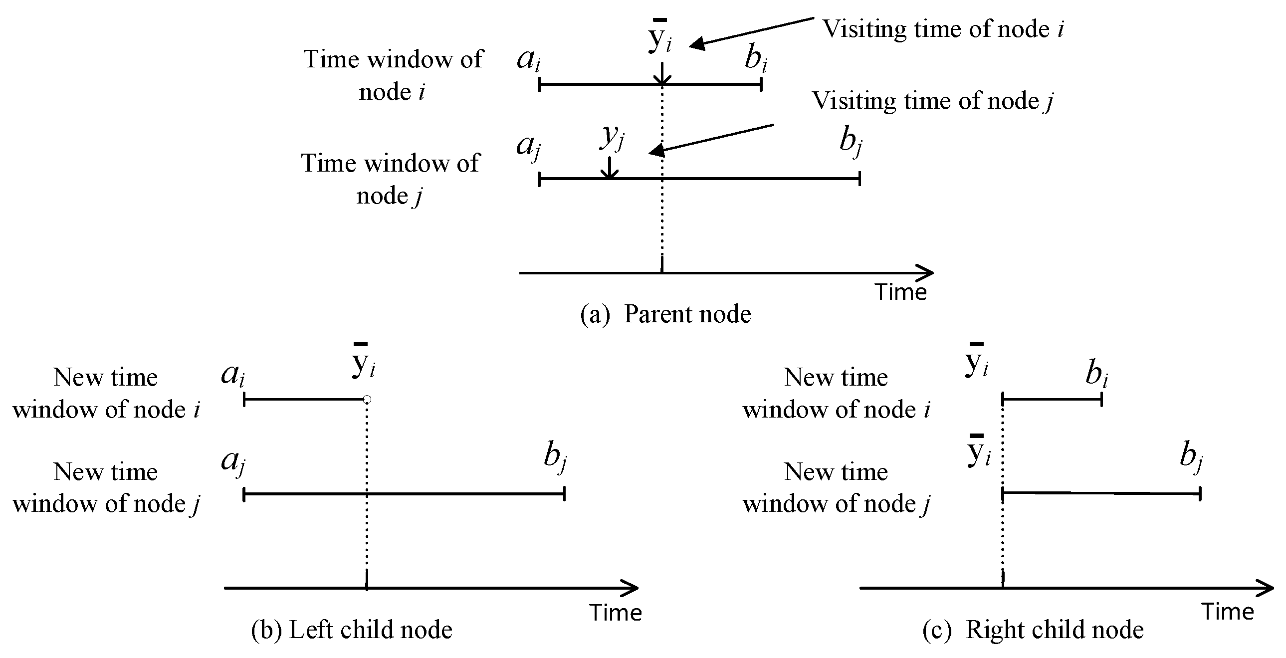
For the second case, the parent node is divided into two child nodes as follows: In the left child node, we narrow the time window of node i to $[a_i,\overline{y_i})$. Since node i must be visited before node j, node j has its time window adjusted accordingly to $[a_i,b_j]$. This child node inherits all columns from the parent node that satisfy these two time window constraints to initialize its RLMP. In the right child node, we restrict the time window of node i to $[\overline{y_i},b_i]$. Similarly, node j has its time window narrowed to $[\overline{y_i},b_j]$. This child node also retains all columns from the parent node that meet these two time window constraints to initialize its RLMP. Figure 7 visually depicts the time window branching strategy.

4.5. Bounding Strategy

A good upper bound helps eliminate unnecessary branching nodes and reduces the size of the node tree, thereby saving the algorithm’s search time. To this end, once the relaxed master problem at each search tree node is solved to optimality using column generation, all identified RLMP variables are converted back to their 0–1 integer constraints, and the pairwise temporal constraints (31) are re-included in the model. The resulting model is then solved through an integer programming solver. Obviously, the obtained solution is a feasible one for the considered problem. Therefore, if the objective function value of this feasible solution is less than the current upper bound, the current upper bound is adjusted to this improved value. And, nodes in the branching tree with lower bounds exceeding the new upper bound are removed.

5. Numerical Simulations

To assess the effectiveness of our proposed algorithm and analyze the impact of various factors on transportation costs, we perform thorough experiments using a series of randomly generated instances. This section presents the findings from these experiments. We begin by describing the instance generation scheme and detailing our experiment setup. Following this, we compare the performance of our algorithm with the genetic algorithm and tabu search algorithm, which are adapted from the works of Yu et al. [16] and Zhang et al. [18], respectively. Next, we justify the adoption of the enhancement techniques. Finally, we undertake a rigorous comparative and sensitivity analysis to obtain valuable insights for management.

5.1. Test Instance Generation and Experimental Configuration

Due to the lack of existing benchmarks for our studied problem, we randomly create new instances using methods similar to those proposed by Zhang et al. [14] and Nossack and Pesch [30], but with adjustments made to better fit the characteristics of our problem. Specifically, the service area of transportation enterprises is assumed to be a square region with each side measuring 180 km. The terminal, depot, and customer locations are randomly generated within this area. The Euclidean distance between two points serves as the driving distance between them. The average driving speed of all trucks is assumed to be 60 km/h. The time required to pack goods into containers or unpack goods from containers is randomly generated, spanning from 0 to 1 h. The time to load/unload containers onto/from trucks is randomly generated within [0.1, 0.2] h. The number of empty containers initially available at the depot is generated randomly. The length of each time window is fixed at 3 h, and the working limit is 8 h. Fixed costs for container trucks with capacities of 1 TEU and 2 TEU are set at 400 CNY and 450 CNY, respectively. The unladen weight of trucks with capacities of 1 TEU and 2 TEU are set at 11 t and 15 t, respectively. The unladen weights of trucks with capacities of 1 TEU and 2 TEU are set at 11 t and 15 t, respectively. The weights of empty 20 ft and 40 ft containers are set to 2 t and 3.5 t, respectively. The weight of goods contained in 20 ft containers is randomly generated in the range of [18 t, 20 t], while for 40 ft containers, it is in the range of [20 t, 23.5 t]. Other parameters which are used to compute the fuel consumption and the carbon emissions are provided in

Table 3. Parameters related to fuel consumption the carbon emissions.

Parameter	Value
Fuel cost per liter $P_{fuel}$	8 CNY/L
Carbon emissions per liter $\varphi$	2.23 kg/L
The carbon tax $C_{tax}$	0.05 CNY/kg
Engine-specific coefficient $\xi$	0.00021 L/s
Speed-specific coefficient $\lambda$	$1.82\times {10}^{-7}$ Ls2/m3
Weight-specific coefficient $\theta$	$8.40\times {10}^{-9}$ L/(m * kg)

[31,32].

To evaluate the algorithm’s performance in solving small-, medium-, and large-scale problems, this study compares the branch-and-price algorithm with the tabu search algorithm and genetic algorithm. The maximum runtime for the branch-and-price algorithm is set to 1 h. The population size, crossover probability, and mutation probability for the genetic algorithm are set to 30, 0.4, and 0.1, respectively. The neighborhood size for the tabu search algorithm is set to 30, and the tabu tenure is set to 10. The maximum number of iterations for the tabu search algorithm and the genetic algorithm is set to 20 times the total number of container transportation requests. The tabu search and genetic algorithm are repeated 10 times for each test case. All algorithms are coded in MATLAB 2021a. At each iteration of column generation, the RLMP is solved by CPLEX 12.10. The experiments are performed on a PC running Windows 10, equipped with an Intel Core i5 processor at 1.6 GHz and 8 GB of RAM.

5.2. Computational Results

5.2.1. Results of Small- and Medium-Scale Instances

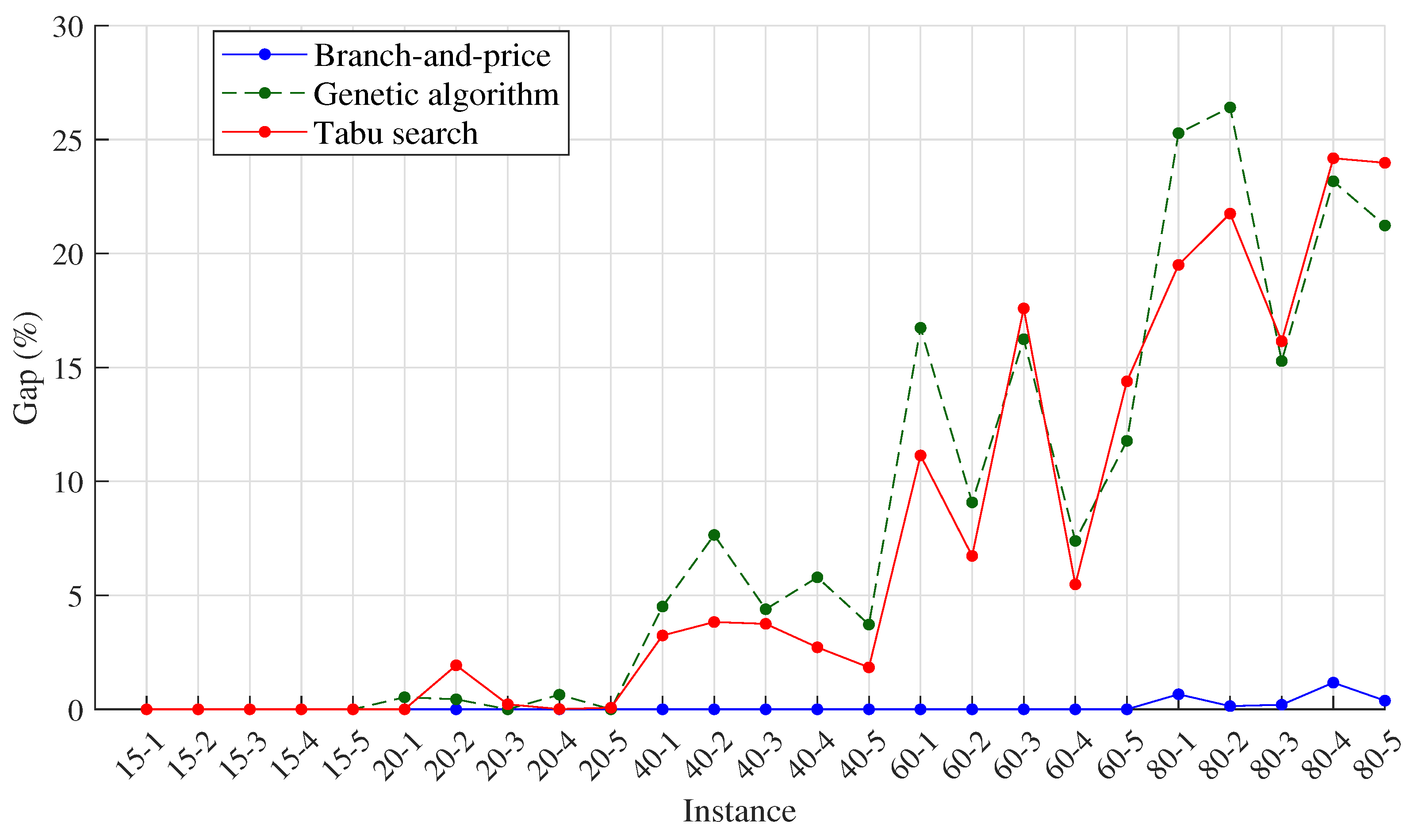
A collection of small- and medium-sized instances is created to validate the effectiveness of the proposed algorithm with respect to computation time and solution quality. The problem sizes tested in this section range from 15 to 80 requests. For each problem size, five instances are created. The experimental results are shown in

Table 4. Comparative results for small- and medium-sized instances.

Ins	LB	Branch-and-Price			Genetic Algorithm			Tabu Search
		Obj (CNY)	CPU (s)	Gap (%)	Obj (CNY)	CPU (s)	Gap (%)	Obj (CNY)	CPU (s)	Gap (%)
15-1	8005.54	8005.54	2.2	0	8005.54	153.1	0	8005.54	100.3	0
15-2	6990.45	6990.45	1.4	0	6990.45	126.2	0	6990.45	88.4	0
15-3	7573.85	7573.85	1.1	0	7573.85	111.3	0	7573.85	85.5	0
15-4	7991.12	7991.12	0.9	0	7991.12	160.5	0	7991.12	80.4	0
15-5	6762.68	6762.68	2.2	0	6762.68	148.0	0	6762.68	86.3	0
Average	7464.73	7464.73	1.6	0	7464.73	139.8	0	7464.73	88.2	0
20-1	11,068.27	11,068.27	3.3	0	11,126.67	219.7	0.53	11,068.27	199.9	0
20-2	8485.57	8485.57	12.1	0	8523.27	220.1	0.44	8649.01	154.9	1.93
20-3	9961.17	9961.17	4.4	0	9961.17	212.2	0	9982.62	158.2	0.22
20-4	10,074.39	10,074.39	15.2	0	10,138.66	206.0	0.64	10,075.77	153.1	0.01
20-5	8876.97	8876.97	67.3	0	8876.97	199.3	0	8883.50	166.4	0.07
Average	9693.27	9693.27	20.5	0	9725.35	211.5	0.32	9731.83	166.5	0.45
40-1	18,133.06	18,133.06	81.3	0	18,950.32	830.5	4.51	18,720.71	556.2	3.24
40-2	16,692.86	16,692.86	122.9	0	17,969.90	749.3	7.65	17,331.51	519.8	3.83
40-3	19,205.73	19,205.73	119.6	0	20,048.78	687.6	4.39	19,926.12	467.1	3.75
40-4	17,958.27	17,958.27	113.5	0	18,997.52	673.9	5.79	18,446.95	491.9	2.72
40-5	19,684.70	19,684.70	274.7	0	20,417.10	628.2	3.72	20,046.11	491.1	1.84
Average	18,334.92	18,334.92	142.4	0	19,276.72	713.9	5.21	18,894.28	505.2	3.07
60-1	27,357.29	27,357.29	312.1	0	31,936.90	1439.5	16.74	30,404.16	1167.2	11.14
60-2	25,625.43	25,625.43	141.5	0	27,952.67	1338.1	9.08	27,349.41	1201.1	6.73
60-3	25,623.82	25,623.82	820.2	0	29,785.62	1416.8	16.24	30,130.46	1105.5	17.59
60-4	24,820.74	24,820.74	1032.7	0	26,655.37	1590.5	7.39	26,182.11	1134.8	5.48
60-5	25,846.78	25,846.78	1593.2	0	28,892.49	1421.6	11.78	29,566.73	1001.0	14.39
Average	25,854.81	25,854.81	779.9	0	29,044.61	1441.3	12.2	28,726.57	1121.9	11.07
80-1	31,348.31	31,554.81	3600.0	0.66	39,272.93	3375.7	25.28	37,459.72	1943.7	19.50
80-2	30,166.71	30,208.79	3600.0	0.14	38,134.08	2437.9	26.41	36,727.26	1887.2	21.75
80-3	29,774.46	29,834.54	3600.0	0.20	34,324.77	2351.6	15.28	34,583.22	1717.2	16.15
80-4	30,359.36	30,715.00	3600.0	1.17	37,393.83	2191.6	23.17	37,699.13	1637.3	24.18
80-5	33,303.11	33,429.26	3600.0	0.38	40,374.00	2234.6	21.23	41,288.75	1610.6	23.98
Average	30,990.39	31,148.48	3600.0	0.51	37,899.92	2518.3	22.28	37,551.61	1759.2	21.11

. In the table, “Ins” denotes the problem number, “LB” represents the lower bound achieved by the branch-and-price algorithm, “Obj” displays the best objective value (in CNY) found by each algorithm, “CPU” indicates the (average) time (in seconds) taken by the algorithms, and “Gap” measures the percentage difference between each algorithm’s best solution and the lower bound, which is computed by $(Obj-LB)/LB\ast 100\%$. In the provided table, the best results for each metric are marked in bold for easy identification.

From the Gap indicator in the table, it is evident that the branch-and-price algorithm can exactly solve problems with 60 requests within 1 h. For cases where the optimal solution is not found, the Gap between the feasible solution and the lower bound of the problem does not exceed 1.2%, indicating that the feasible solutions obtained by our proposed algorithm are of exceptionally high quality. According to the CPU indicator, the runtime of the branch-and-price algorithm significantly increases with the problem size. For larger problems, the computational complexity leads to runtimes close to the preset limit (e.g., CPU times for cases with 80 requests are 3600 s). This phenomenon is due to the fact that after Dantzig–Wolfe decomposition, the pricing subproblems remain NP-hard. As the problem size increases, the time required to accurately solve the subproblems inevitably increases. Therefore, while the exact branch-and-price algorithm has very high solution quality, the extensive computational time cost is the main limiting factor for solving large-scale problems.

In comparison to the branch-and-price algorithm, the results obtained by the tabu search and genetic algorithms are notably inferior. Although these two heuristic algorithms consume relatively less time when solving problem sizes larger than 60 and have certain advantages in solving efficiency, their solution quality is significantly worse than that of the branch-and-price algorithm, as indicated by the Gap values. Figure 8 also provides a visual comparison of the Gap values between these two heuristic algorithms and our proposed algorithm, clearly highlighting the disparities in the performance of the heuristic methods. Furthermore, the Gap values start low for smaller instances but increase significantly for larger ones, indicating a decline in the solution quality as the problem size increases. For example, as the problem size increases from 15 to 80, the average Gap for the tabu search algorithm rises from 0 to 21.11%, and for the genetic algorithm, it increases from 0 to 22.28%. In contrast, the average Gap for the branch-and-price algorithm is always 0 for problem sizes up to 60 and only reaches 0.51% when the problem size is 80. This clearly demonstrates that the tabu search algorithm and the genetic algorithm struggle with maintaining the solution quality when handling small-scale and medium-scale problems. In summary, the branch-and-price algorithm is superior to heuristic algorithms in terms of solution quality but can be computationally expensive for larger instances. This highlights the need to balance computational efficiency and solution quality when solving larger-scale problems.

5.2.2. Results of Large-Scale Instances

As shown in Section 5.2.1, although the branch-and-price algorithm (hereafter referred to as the exact branch-and-price algorithm) demonstrates its superiority in solving small- and medium-scale instances, its efficiency diminishes as the problem size grows. This limitation highlights the need for a more practical approach to handle larger instances. To this end, we construct a heuristic branch-and-price algorithm based on the exact version to obtain high-quality feasible solutions for large-scale problems. The core of this approach lies in using a heuristic label-setting algorithm instead of an exact label-setting algorithm to heuristically solve the pricing subproblem. Experiments are conducted with instances of 100, 120, and 160 container transportation requests, and the results are shown in

Table 5. Comparative results for large-scale instances.

Ins	Branch-and-Price		Genetic Algorithm			Tabu Search
	Obj (CNY)	CPU (s)	Obj (CNY)	CPU (s)	Gap (%)	Obj (CNY)	CPU (s)	Gap (%)
100-1	41,235.11	3600.0	48,204.36	2627.0	16.90	48,051.17	2534.5	16.53
100-2	38,424.29	3600.0	49,189.31	2790.5	28.02	47,151.14	2282.7	22.71
100-3	39,112.85	3600.0	46,052.86	2856.1	17.74	44,103.13	2421.2	12.76
100-4	45,983.66	3600.0	48,937.88	2708.4	6.42	51,213.51	2233.4	11.37
100-5	40,316.55	3600.0	48,937.88	2654.0	21.38	48,153.26	2266.5	19.44
Average	41,014.49	3600.0	48,264.46	2727.2	18.09	47,734.44	2347.7	16.56
120-1	46,961.14	3600.0	56,308.80	4092.8	19.91	55,994.75	3104.3	19.24
120-2	47,503.36	3600.0	59,026.46	3769.5	24.26	55,800.31	3263.8	17.47
120-3	47,436.77	3600.0	57,838.13	3511.6	21.93	56,490.31	3157.0	19.09
120-4	47,667.23	3600.0	57,335.73	3233.8	20.28	56,553.33	3251.5	18.64
120-5	51,068.30	3600.0	62,473.83	2833.3	22.33	60,457.96	3183.0	18.39
Average	48,127.36	3600.0	58,596.59	3488.2	21.74	57,059.33	3191.9	18.56
160-1	61,929.31	3600.0	79,455.31	6590.3	28.30	74,171.63	5227.3	19.77
160-2	63,367.66	3600.0	77,391.17	5267.4	22.13	75,331.57	5457.8	18.88
160-3	64,555.89	3600.0	83,217.71	8071.4	28.91	80,944.50	5130.9	25.39
160-4	61,750.05	3600.0	79,482.28	7853.2	28.72	75,365.98	5311.9	22.05
160-5	67,466.78	3600.0	85,316.26	8210.3	26.46	81,807.78	5289.2	21.26
Average	63,813.94	3600.0	80,972.54	7198.5	26.90	77,524.29	5283.4	21.47

, where Gap represents the percentage difference between the results of each algorithm and those produced by the heuristic branch-and-price algorithm. Other column headings are consistent with those in the previous section.

The experimental results show that the heuristic branch-and-price algorithm achieves notably superior results compared to both the tabu search and genetic algorithms. For instance, in cases with 100 requests, the average Gap between the results of the tabu search algorithm and those of the heuristic branch-and-price algorithm is 16.56%, while for the genetic algorithm, it is 18.09%. Similarly, as the problem size increases, the Gap indicator generally shows an upward trend. A reasonable explanation for this phenomenon is as follows. The genetic algorithm searches for solutions through a limited population. Although crossover and mutation operations promote population evolution, this process is also accompanied by a gradual decline in population diversity. This reduction in diversity often limits the algorithm’s exploratory capability in the search space, causing it to prematurely converge to a local optimal solution. Similarly, the tabu search algorithm may be constrained by the length of the tabu list and the search strategy during its search process. Specifically, a tabu length that is too short may fail to effectively avoid search loops, while a tabu length that is too long may hinder the search process by making it less exploitative and more computationally intensive. Additionally, if the search strategy is not well designed or lacks sufficient flexibility, the tabu search algorithm may struggle to thoroughly and deeply explore promising solutions in the complex solution space, thereby limiting its overall performance in solving large-scale problems.

In conclusion, the heuristic branch-and-price algorithm demonstrates notable advantages over the tabu search and genetic algorithms for large-scale problems. It is capable of producing high-quality solutions more efficiently as the problem size grows, which suggests it is a promising alternative for tackling large-scale ICTs.

5.3. Effectiveness of the Enhancement Strategies

To improve the efficiency of our proposed exact branch-and-price algorithm for small- and medium-scale instances, we implement strategies including the heuristic label-setting algorithm and decremental state-space relaxation to accelerate the column generation process. Additionally, we introduce a bounding scheme to effectively prune nodes. To assess the effectiveness of these enhancements, we select three sets of instances with problem sizes of 15, 20, and 40. We then compare the performance of the proposed exact branch-and-price algorithm with the basic branch-and-price algorithm without enhancement strategies. The experimental results are shown in

Table 6. Performance comparison: proposed vs. basic branch-and-price algorithms.

Ins	Proposed Exact Branch-and-Price			Basic Branch-and-Price
	Obj (CNY)	CPU (s)	Node	Obj (CNY)	CPU (s)	Node
15-1	8005.54	2.2	1	8005.54	18.3	1
15-2	6990.45	1.4	1	6990.45	23.2	1
15-3	7573.85	1.1	1	7573.85	6.9	1
15-4	7991.12	0.9	1	7991.12	14.9	1
15-5	6762.68	2.2	1	6762.68	22.2	1
20-1	11,068.27	3.3	1	11,068.27	328.9	1
20-2	8485.57	12.1	1	8485.57	135.2	1
20-3	9961.17	4.4	1	9961.17	136.9	1
20-4	10,074.39	15.2	9	10,074.39	412.8	9
20-5	8876.97	67.3	31	8876.97	2617.2	35
40-1	18,133.06	81.3	1	-	-	-
40-2	16,692.86	122.9	3	-	-	-
40-3	19,205.73	119.6	3	-	-	-
40-4	17,958.27	113.5	1	-	-	-
40-5	19,684.70	274.7	1	-	-	-

“-”: the corresponding algorithm fails to find a feasible solution.

. The column labeled “Node” indicates the number of nodes explored by each algorithm, while the other column headings maintain the same definitions as those in the previous section.

The proposed exact branch-and-price algorithm achieves a considerable reduction in computation time compared to the basic version. For example, in instances with 15 requests, all of which are exactly solved by examining only the root node, the enhanced performance of the branch-and-price algorithm is primarily driven by the integration of the heuristic label-setting algorithm and the decremental state-space relaxation, both of which are designed to speed up the column generation process. As a result, these enhancements collectively lead to a marked acceleration of the proposed exact branch-and-price algorithm. Observations from the node metric, for instance, 20-5, indicate that our proposed algorithm searches fewer nodes than the basic version. This suggests that the introduction of the bounding strategy effectively lowers the number of nodes searched and shortens computation time. Furthermore, for instances involving over 40 requests, the basic branch-and-price algorithm is unable to provide a feasible solution within an hour, highlighting the inefficiency and impracticality of using an exact algorithm to solve pricing subproblems in medium instances. In summary, the results confirm that the incorporation of enhancement strategies results in a substantial improvement in the efficiency of the branch-and-price approach.

5.4. Sensitivity Analysis

In this subsection, we will analyze the effects of critical parameters on the total transportation cost.

5.4.1. Impact of the Initial Number of Empty Containers at the Depot

To explore how the initial inventory of empty containers at the depot affects the total transportation cost, this paper selects instances of different scales: 15-5, 20-4, 40-1, and 60-4 for testing. We keep the number of 20 ft empty containers at the depot unchanged and gradually increase the initial number of 40 ft empty containers. For each scenario, the total transportation costs are computed.

Table 7. Impact of the initial number of empty containers at the depot on total transportation cost.

Number of Empty Containers	Total Transportation Cost (CNY)
	Ins 15-5	Ins 20-4	Ins 40-1	Ins 60-4
0	6779.16	10,154.07	18,211.60	24,954.44
1	6762.68	10,074.39	18,133.06	24,905.60
2	6762.68	10,074.39	18,103.62	24,858.94
3	6762.68	10,074.39	18,103.62	24,820.74
4	6762.68	10,074.39	18,103.62	24,820.74

and Figure 9 illustrate the variation in total transportation costs as the quantity of 40 ft empty containers changes.

As shown in Figure 9, an increase in the number of empty containers leads to a reduction in the total transportation cost. Increasing the initial inventory of empty containers at the depot by one unit each time reduces the transportation cost, but the impact on cost savings is relatively minor, amounting to less than 1%. Notably, for instance, 60-4, the total cost can be reduced by 0.54% when the initial quantity of empty containers kept at the depot increases from 0 to 3. Moreover, after the number of empty containers reaches a certain level, the total transportation cost levels off and does not decrease further. This indicates that once the depot has a sufficient number of empty containers, further increasing the number of empty containers does not provide further reductions in the transportation cost, reflecting the principle of diminishing marginal returns. This experiment suggests that having a large stock of empty containers is not necessarily economically beneficial. The truck firm needs to figure out the ideal inventory of empty containers based on factors such as their business volume, container purchase costs, and other relevant considerations.

5.4.2. Impact of Truck Fleet Configuration

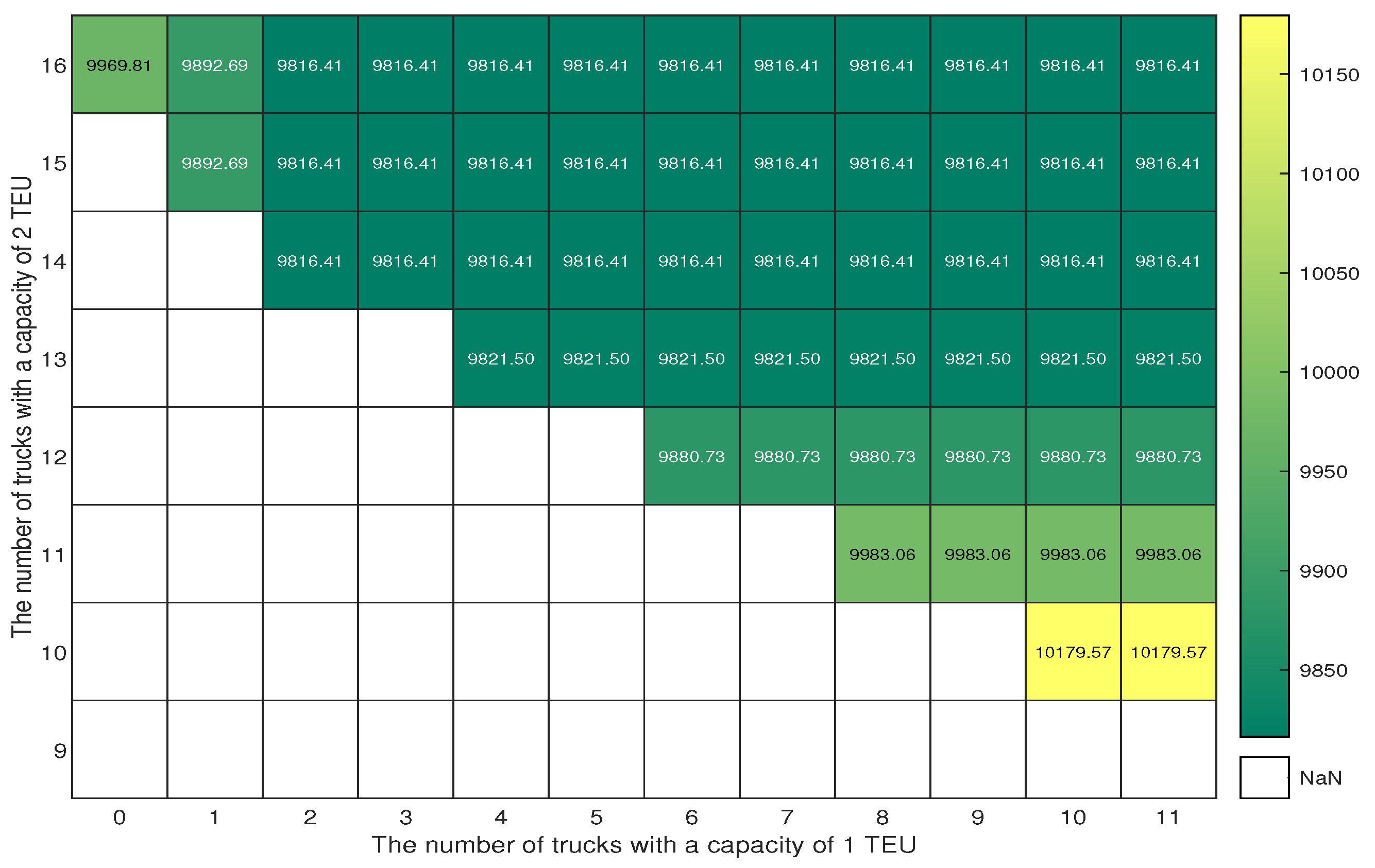
We select instance 40-1 as a representative case to analyze the impact of truck types on the total transportation cost, as well as fuel and carbon emission costs. Figure 10 and Figure 11 present heatmaps that clearly illustrate the distribution of these costs under different combinations of trucks with capacities of 1 TEU and 2 TEU.

Data from the figures reveal that using only trucks with a capacity of 2 TEU typically results in greater total costs, including higher fuel and carbon emission costs. Alternatively, integrating trucks with a capacity of 1 TEU into the fleet (i.e., adopting a mixed truck fleet) usually reduces the transportation cost. For example, in this instance, introducing a single truck with a capacity of 1 TEU reduces the total cost from 17,169.81 CNY to 17,042.69 CNY. The reason is that incorporating trucks with a 1 TEU capacity provides greater flexibility. When both types of trucks work together, they can more effectively meet diverse container transportation needs and minimize the capacity waste typically associated with trucks with a 2 TEU capacity.

However, this does not imply that simply increasing the number of trucks with a 1 TEU capacity while reducing trucks with a 2 TEU capacity is always the most cost-effective strategy. As shown in Figure 11, cutting the number of trucks with a 2 TEU capacity from 16 to 10 and increasing the number of trucks with a 1 TEU capacity from 0 to 10 leads to a rise in the total transportation cost from 17,169.81 CNY to 18,679.57 CNY. The reason is that the truck with a 2 TEU capacity can handle two 20 ft containers simultaneously. When there are not enough of these trucks, more trucks with a capacity of 1 TEU are required to complete the transportation requests, some of which could have been consolidated and managed by fewer trucks with a capacity of 2 TEU. This results in a higher transportation cost.

Thus, the truck fleet configuration has a great influence on the costs. In the case of instance 40-1, the optimal configuration involves 2 trucks with a 1 TEU capacity and 14 trucks with a 2 TEU capacity. Any reduction in the number of either type of truck results in an increase in fuel and carbon emission costs, as well as the total cost. The optimal truck combination should be determined based on factors such as business volume, container size, truck availability, and so on.

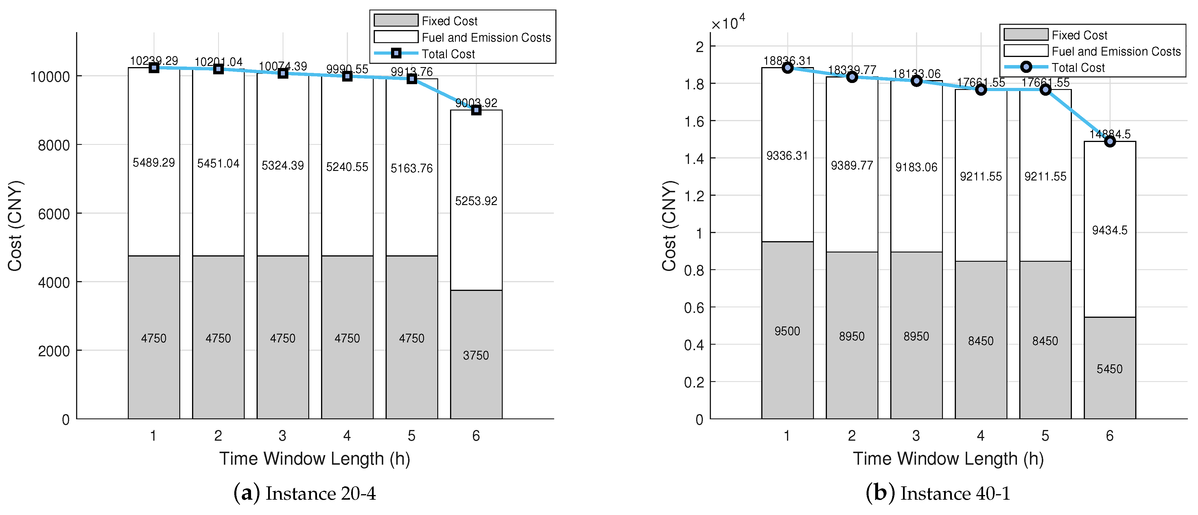
5.4.3. Impact of Time Window Length

In this subsection, we attempt to explore the influence of time window length on costs. For this purpose, instances 20-4 and 40-1 are selected, and the time window length is gradually increased from 1 h to 6 h. Figure 12 shows the corresponding fixed cost, fuel and carbon emission costs, and total transportation cost.

As shown in Figure 12, the total transportation cost decreases as the time window lengthens. Specifically, when the time window length increases from 1 h to 6 h, the total cost for instances 20-4 and 40-1 decrease by 12.06% and 20.97%, respectively. The reason for this phenomenon lies in that a wider allowable service beginning time provides the truck firm with greater flexibility. This increased flexibility broadens the range of feasible routing and scheduling options and often allows for the selection of more cost-efficient routes from a larger set of choices.

From the perspective of cost composition, fixed costs decrease gradually with an increase in the time window length while fuel and carbon emission costs may fluctuate up and down. For example, in instance 40-1, when the time window length is extended from 2 h to 3 h, the fuel and carbon emission costs decrease from 9389.77 CNY to 9183.06 CNY. However, when the time window is further extended from 3 h to 4 h, these costs conversely increase from 9183.06 CNY to 9211.55 CNY. This is primarily because the truck’s fixed cost is comparatively higher than the fuel and carbon emission costs per unit of route length. Therefore, cutting down the number of dispatched trucks becomes a key objective, even if it means increasing route lengths. Despite these fluctuations, the reduction in fixed costs often outweighs the increase in fuel and carbon emission costs, leading to an overall reduction in the total cost. The drayage firm might therefore negotiate with customers for longer time windows, which allows them to achieve savings in the total transportation cost.

6. Conclusions

This study addresses the inland container transportation problem, which factors in the challenges posed by the limited availability of empty containers, the multiple container sizes, and the necessity to minimize fuel consumption and carbon emissions. This research introduces an innovative graph modeling technique, which simplifies the formulation of the problem into a mixed-integer programming model. To tackle this model efficiently, a tailored branch-and-price algorithm is devised. The validity and effectiveness of the approach are demonstrated through extensive numerical experiments on randomly generated instances.

The experiments offer several important findings and practical management insights. Firstly, the proposed exact branch-and-price algorithm can exactly solve problems with approximately 60 container transportation requests within 1 h. For larger-scale problems, the heuristic branch-and-price algorithm, adapted from the exact version, delivers superior results compared to the genetic algorithm and the tabu search algorithm. Secondly, as the initial stock of empty containers at the depot increases, the total transportation cost decreases. Each additional empty container yields a marginal cost reduction of less than 1%, and there is a noticeable diminishing marginal effect. Thirdly, the total transportation cost including fuel and carbon emission costs can be saved by reasonably configuring different types of trucks and fully utilizing their respective advantages. Last but not least, wider time windows can potentially be advantageous for container transportation operations, offering operators increased flexibility and cost savings.

The implications of this research go beyond academic contributions. Policymakers can use these findings to support the development of regulations that promote sustainable logistics practices, encouraging better management of empty container inventories and truck fleets. This aligns with efforts to meet carbon reduction goals. For logistics companies, adopting these optimization strategies will enable them to meet stricter environmental regulations while maintaining operational efficiency. Moreover, extending time windows also offers an important opportunity to enhance service flexibility, which is particularly beneficial in competitive markets.

In terms of future research, several avenues are worth exploring. The speed of trucks is subject to numerous factors including traffic volume, weather conditions, and infrastructure. Thus, considering the problem within a dynamic setting would be valuable. Additionally, electric and hybrid trucks are increasingly viable due to advances in battery technology and charging infrastructure. These trucks are able to substantially lower carbon emissions and operational costs. An additional important area for investigation is the impact of regulatory constraints on container transportation. Gaining insights into how various policies and regulations influence operational practices can lead to more effective logistics strategies. Therefore, investigating the integration of electric and hybrid trucks, their associated working practices, and regulatory limitations into the ICT is another promising research avenue, which could contribute to the development of more sustainable and cost-effective container logistics.

References

1. Springel, K. Network externality and subsidy structure in two-sided markets: Evidence from electric vehicle incentives. Am. Econ. J. Econ. Policy 2021, 13, 393–432. [Google Scholar] [CrossRef]
2. Pan, X.; Wang, M.; Li, M. Low-carbon policy and industrial structure upgrading: Based on the perspective of strategic interaction among local governments. Energy Policy 2023, 183, 113794. [Google Scholar] [CrossRef]
3. Available online: https://ww2.arb.ca.gov/resources/fact-sheets/advanced-clean-fleets-regulation-detailed-drayage-truck-requirements (accessed on 2 October 2024).
4. Johanson, G.; Svedberg, U. A novel method for pre-ventilation of shipping containers. Int. J. Hyg. Environ. Health 2020, 230, 113626. [Google Scholar] [CrossRef] [PubMed]
5. Available online: https://www.boomandbucket.com/blog/how-much-storage-is-a-container-costs (accessed on 3 October 2024).
6. Chung, K.H.; Ko, C.S.; Shin, J.Y.; Hwang, H.; Kim, K.H. Development of mathematical models for the container road transportation in Korean trucking industries. Comput. Ind. Eng. 2007, 53, 252–262. [Google Scholar] [CrossRef]
7. Vidović, M.; Radivojević, G.; Raković, B. Vehicle routing in containers pickup up and delivery processes. Procedia Soc. Behav. Sci. 2011, 20, 335–343. [Google Scholar] [CrossRef]
8. Bruglieri, M.; Mancini, S.; Peruzzini, R.; Pisacane, O. The multi-period multi-trip container drayage problem with release and due dates. Comput. Oper. Res. 2021, 125, 105102. [Google Scholar] [CrossRef]
9. Bustos-Coral, D.; Costa, A.M. Drayage routing with heterogeneous fleet, compatibility constraints, and truck load configurations. Transp. Res. Part E Logist. Transp. Rev. 2022, 168, 102922. [Google Scholar] [CrossRef]
10. Zhang, R.; Yun, W.Y.; Kopfer, H. Multi-size container transportation by truck: Modeling and optimization. Flex. Serv. Manuf. J. 2015, 27, 403–430. [Google Scholar] [CrossRef]
11. Funke, J.; Kopfer, H. A model for a multi-size inland container transportation problem. Transp. Res. Part E Logist. Transp. Rev. 2016, 89, 70–85. [Google Scholar] [CrossRef]
12. Moghaddam, M.; Pearce, R.H.; Mokhtar, H.; Prato, C.G. A generalised model for container drayage operations with heterogeneous fleet, multi-container sizes and two modes of operation. Transp. Res. Part E Logist. Transp. Rev. 2020, 139, 101973. [Google Scholar] [CrossRef]
13. Chen, R.; Chen, S.; Cui, H.; Meng, Q. The container drayage problem for heterogeneous trucks with multiple loads: A revisit. Transp. Res. Part E Logist. Transp. Rev. 2021, 147, 102241. [Google Scholar] [CrossRef]
14. Zhang, R.; Yun, W.Y.; Moon, I.K. Modeling and optimization of a container drayage problem with resource constraints. Int. J. Prod. Econ. 2011, 133, 351–359. [Google Scholar] [CrossRef]
15. Zhang, R.; Huang, C.; Wang, J. A novel mathematical model and a large neighborhood search algorithm for container drayage operations with multi-resource constraints. Comput. Ind. Eng. 2020, 139, 106143. [Google Scholar] [CrossRef]
16. Yu, X.; Feng, Y.; He, C.; Liu, C. Modeling and Optimization of Container Drayage Problem with Empty Container Constraints across Multiple Inland Depots. Sustainability 2024, 16, 5090. [Google Scholar] [CrossRef]
17. Fazi, S.; Choudhary, S.K.; Dong, J.X. The multi-trip container drayage problem with synchronization for efficient empty containers re-usage. Eur. J. Oper. Res. 2023, 310, 343–359. [Google Scholar] [CrossRef]
18. Zhang, H.; Zhang, R.; Huang, M.; Shi, H. Modeling and analyses of container drayage transportation problem with the objective of low carbons. In Proceedings of the The 27th Chinese Control and Decision Conference (2015 CCDC), Qingdao, China, 23–25 May 2015; pp. 4654–4658. [Google Scholar]
19. Konstantzos, G.E.; Saharidis, G.K.; Loizidou, M. Development of a model for assessing Greenhouse Gas (GHG) emissions from terminal and drayage operations. Oper. Res. 2017, 17, 807–819. [Google Scholar] [CrossRef]
20. Shiri, S.; Huynh, N. Assessment of US chassis supply models on drayage productivity and air emissions. Transp. Res. Part D Transp. Environ. 2018, 61, 174–203. [Google Scholar] [CrossRef]
21. He, W.; Jin, Z.; Huang, Y.; Xu, S. The inland container transportation problem with separation mode considering carbon dioxide emissions. Sustainability 2021, 13, 1573. [Google Scholar] [CrossRef]
22. Chen, R.; Meng, Q.; Jia, P. Container port drayage operations and management: Past and future. Transp. Res. Part E Logist. Transp. Rev. 2022, 159, 102633. [Google Scholar] [CrossRef]
23. Barth, M.; Younglove, T.; Scora, G. Development of a Heavy-Duty Diesel Modal Emissions and Fuel Consumption Model; Institute of Transportation Studies, UC Berkeley: Berkeley, CA, USA, 2005. [Google Scholar]
24. Barth, M.; Boriboonsomsin, K. Energy and emissions impacts of a freeway-based dynamic eco-driving system. Transp. Res. Part D Transp. Environ. 2009, 14, 400–410. [Google Scholar] [CrossRef]
25. Boland, N.; Dethridge, J.; Dumitrescu, I. Accelerated label setting algorithms for the elementary resource constrained shortest path problem. Oper. Res. Lett. 2006, 34, 58–68. [Google Scholar] [CrossRef]
26. Righini, G.; Salani, M. New dynamic programming algorithms for the resource constrained elementary shortest path problem. Netw. Int. J. 2008, 51, 155–170. [Google Scholar] [CrossRef]
27. Li, J.; Qin, H.; Baldacci, R.; Zhu, W. Branch-and-price-and-cut for the synchronized vehicle routing problem with split delivery, proportional service time and multiple time windows. Transp. Res. Part E Logist. Transp. Rev. 2020, 140, 101955. [Google Scholar] [CrossRef]
28. Huang, N.; Li, J.; Zhu, W.; Qin, H. The multi-trip vehicle routing problem with time windows and unloading queue at depot. Transp. Res. Part E Logist. Transp. Rev. 2021, 152, 102370. [Google Scholar] [CrossRef]
29. Luo, Z.; Qin, H.; Lim, A. Branch-and-price-and-cut for the multiple traveling repairman problem with distance constraints. Eur. J. Oper. Res. 2014, 234, 49–60. [Google Scholar] [CrossRef]
30. Nossack, J.; Pesch, E. A truck scheduling problem arising in intermodal container transportation. Eur. J. Oper. Res. 2013, 230, 666–680. [Google Scholar] [CrossRef]
31. Huang, Y.; Zhao, L.; Van Woensel, T.; Gross, J.P. Time-dependent vehicle routing problem with path flexibility. Transp. Res. Part B Methodol. 2017, 95, 169–195. [Google Scholar] [CrossRef]
32. Fan, H.; Ren, X.; Guo, Z.; Li, Y. Truck scheduling problem considering carbon emissions under truck appointment system. Sustainability 2019, 11, 6256. [Google Scholar] [CrossRef]
Figure 1. The flowchart of this paper.
Processes 12 02231 g001
Figure 2. Visualization of transportation operations for 20 ft containers.
Processes 12 02231 g002
Figure 3. An illustrative example.
Processes 12 02231 g003
Figure 4. Node definitions for container transportation requests.
Processes 12 02231 g004
Figure 5. Nodes representing empty container storage and retrieval from the depot.
Processes 12 02231 g005
Figure 6. Workflow diagram for the proposed branch-and-price algorithm.
Processes 12 02231 g006
Figure 7. Time window branching.
Processes 12 02231 g007
Figure 8. Comparison of Gap values for different algorithms.
Processes 12 02231 g008
Figure 9. Relationship between total cost and the initial number of 40 ft empty containers at the depot.
Processes 12 02231 g009
Figure 10. Heatmap of total transportation cost under different truck fleet configurations.
Processes 12 02231 g010
Figure 11. Heatmap of fuel and carbon emission costs under different truck fleet configurations.
Processes 12 02231 g011
Figure 12. Relationship between time window length and costs.
Processes 12 02231 g012