
An Efficient Method for Identifying Inter-Well Connectivity Using AP Clustering and Graphical Lasso: Validation with Tracer Test Results


Abstract
1. Introduction
2. Background
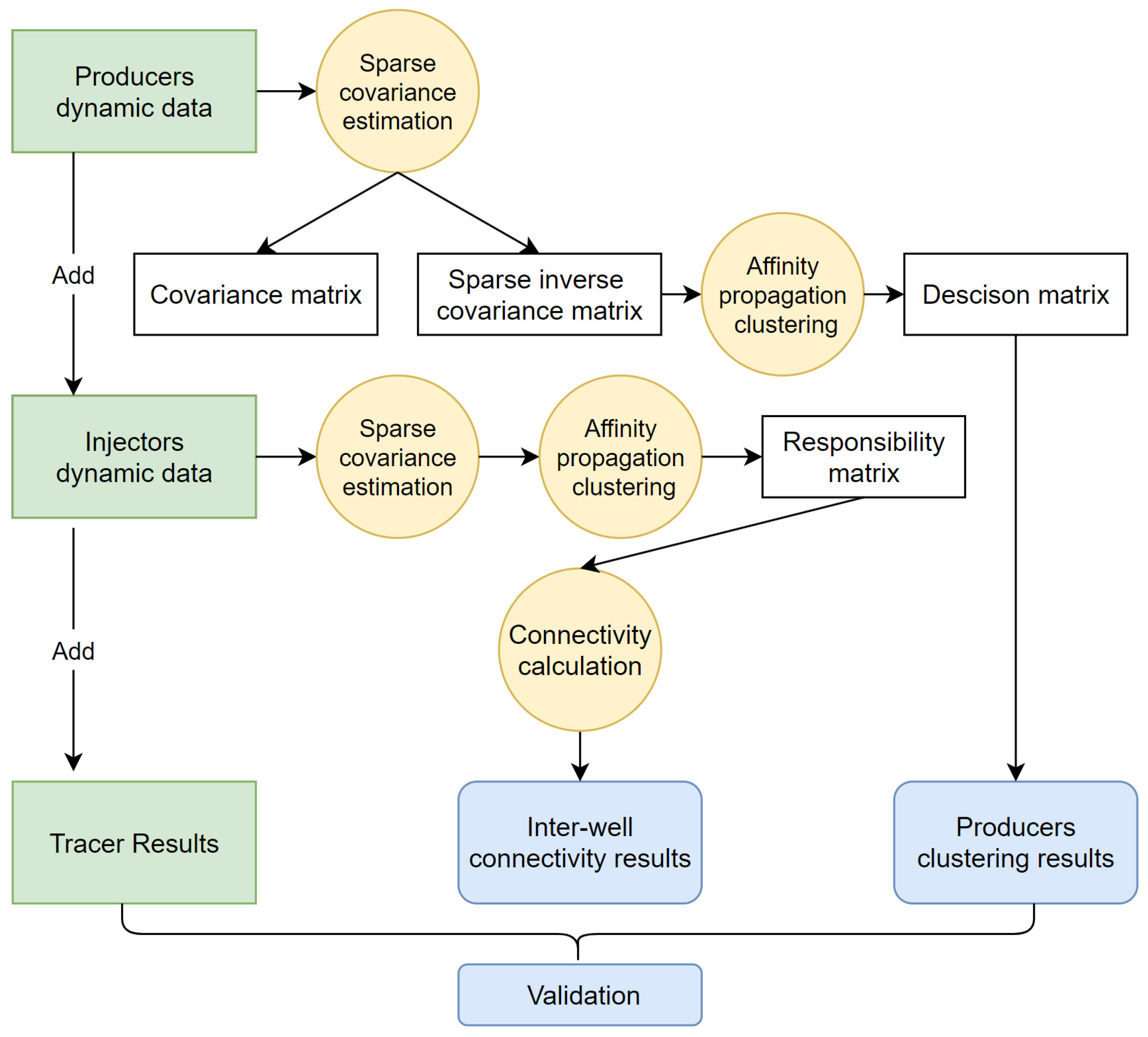
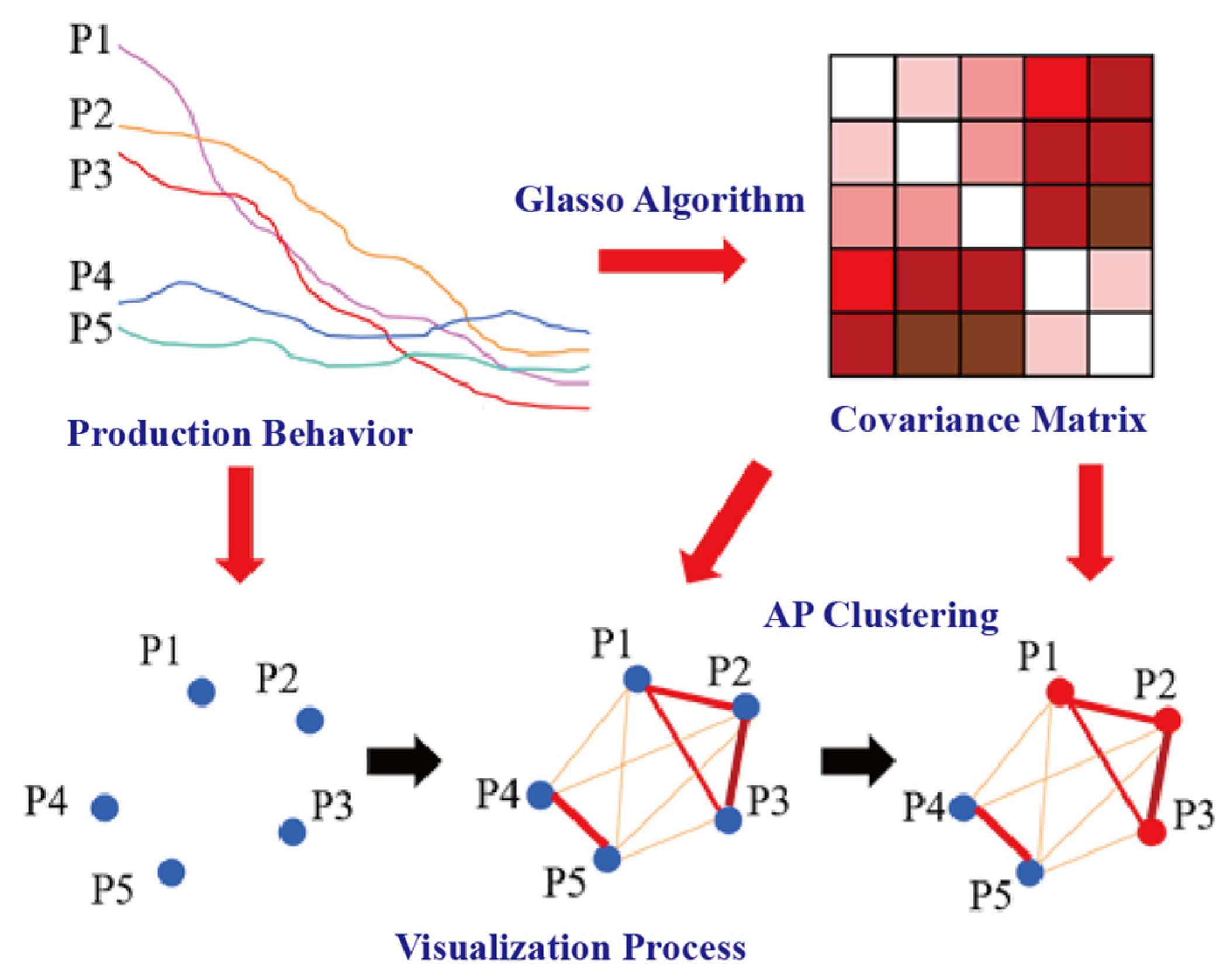
3. Methodology
3.1. Sparse Inverse Covariance Estimation
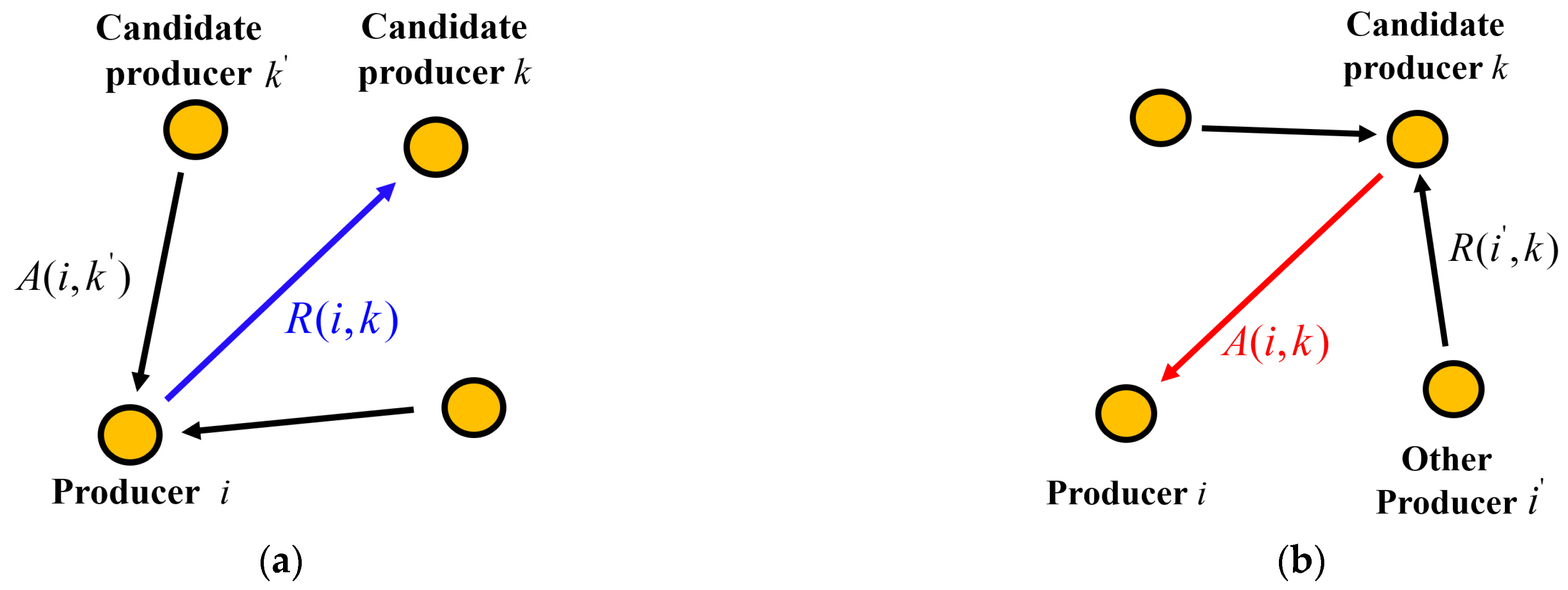
3.2. Affinity Propagation Clustering
3.3. Rapid Evaluation of Injection-Producer Connectivity
4. Results and Discussion
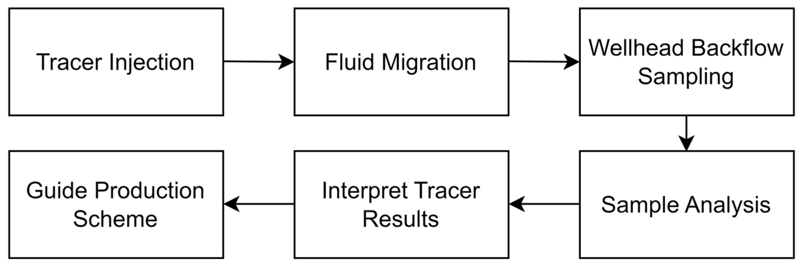
4.1. Tracer Testing
4.2. Results of Reservoir Inter-Well Clustering
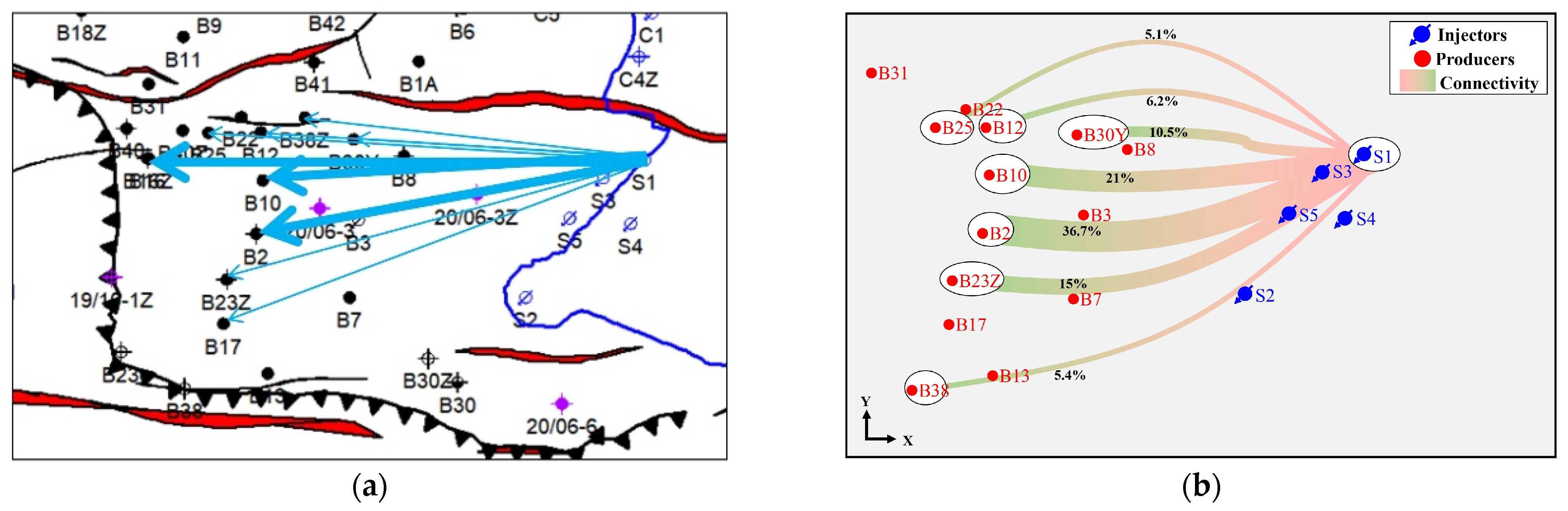
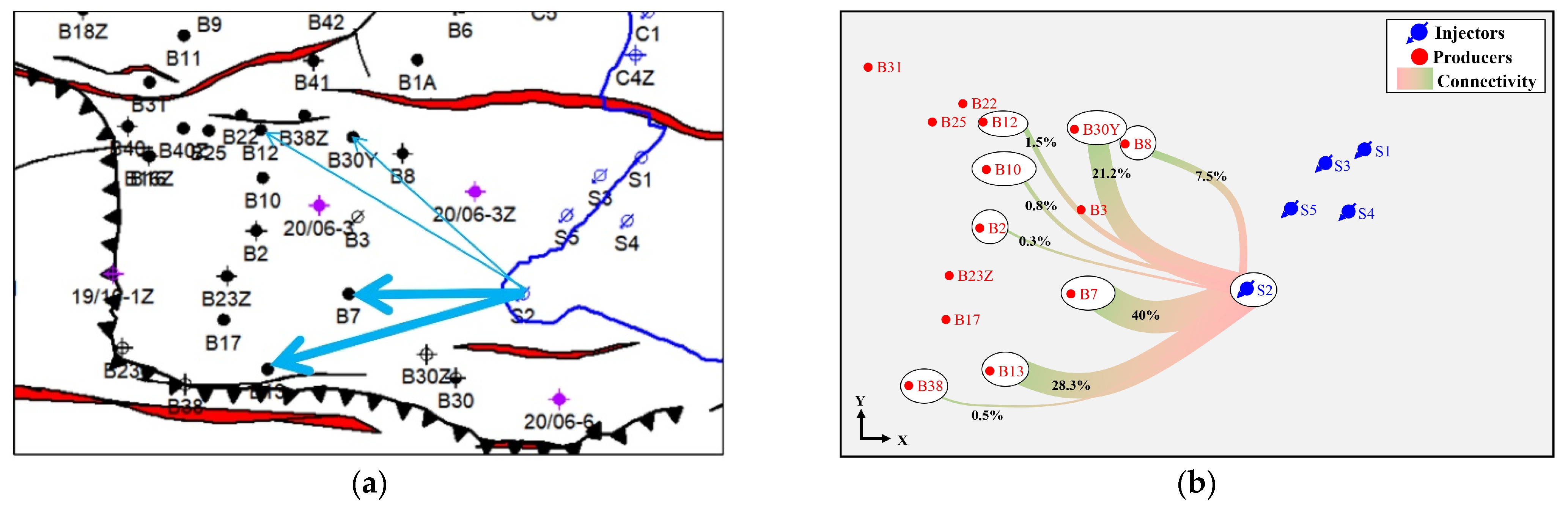
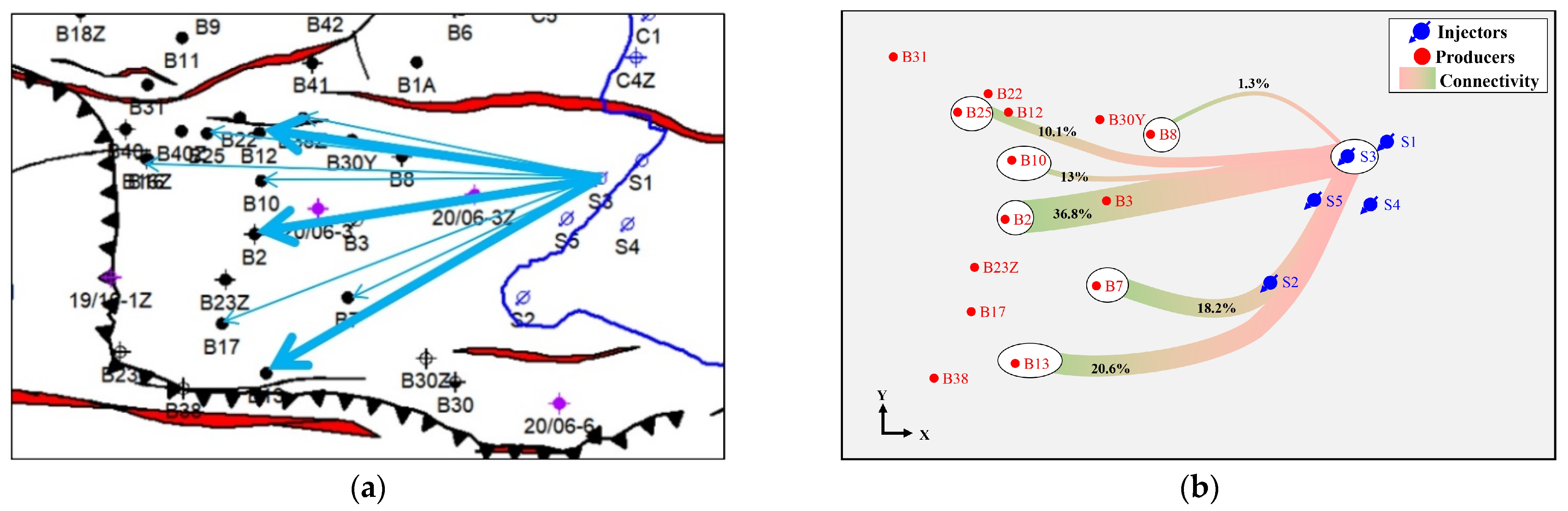
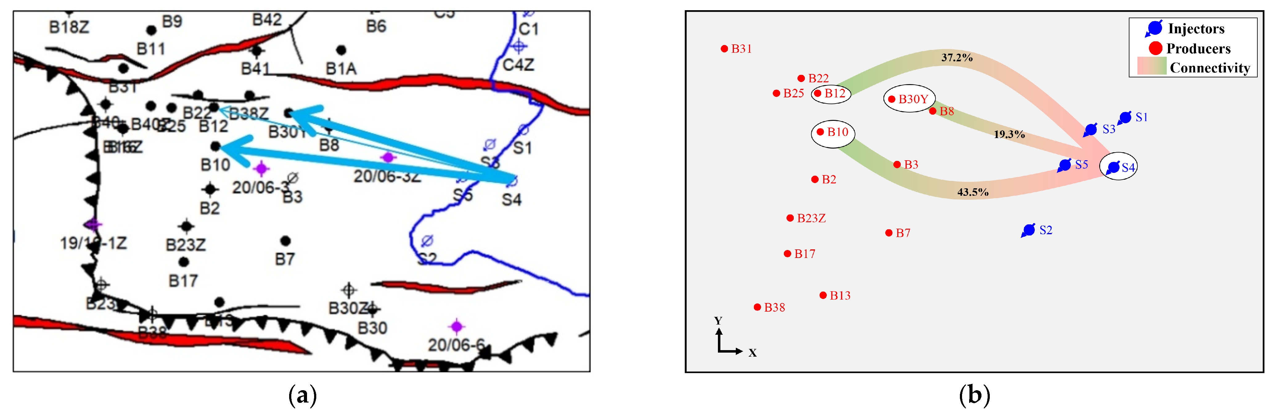
4.3. Evaluation of Inter-Well Connectivity Results
5. Conclusions
- (1)
- For the problem of data default caused by long-term shut-in and data loss, the proposed algorithm can still ensure stability and accuracy. In the validation of calculation results with the tracer test results for the four injectors, the algorithm achieved a precision rate of 79.17% (19 of 24) and a recall rate of 90.48% (19 of 21).
- (2)
- In the 56 calculations of inter-well connectivity, the algorithm was consistent with the tracer test results in 51 instances, yielding an accuracy of 91.07%. Furthermore, the erroneous inter-well connectivity values ranged from a maximum of 0.075 to a minimum of only 0.003, making the overall impact on the assessment of injector connectivity acceptable.
- (3)
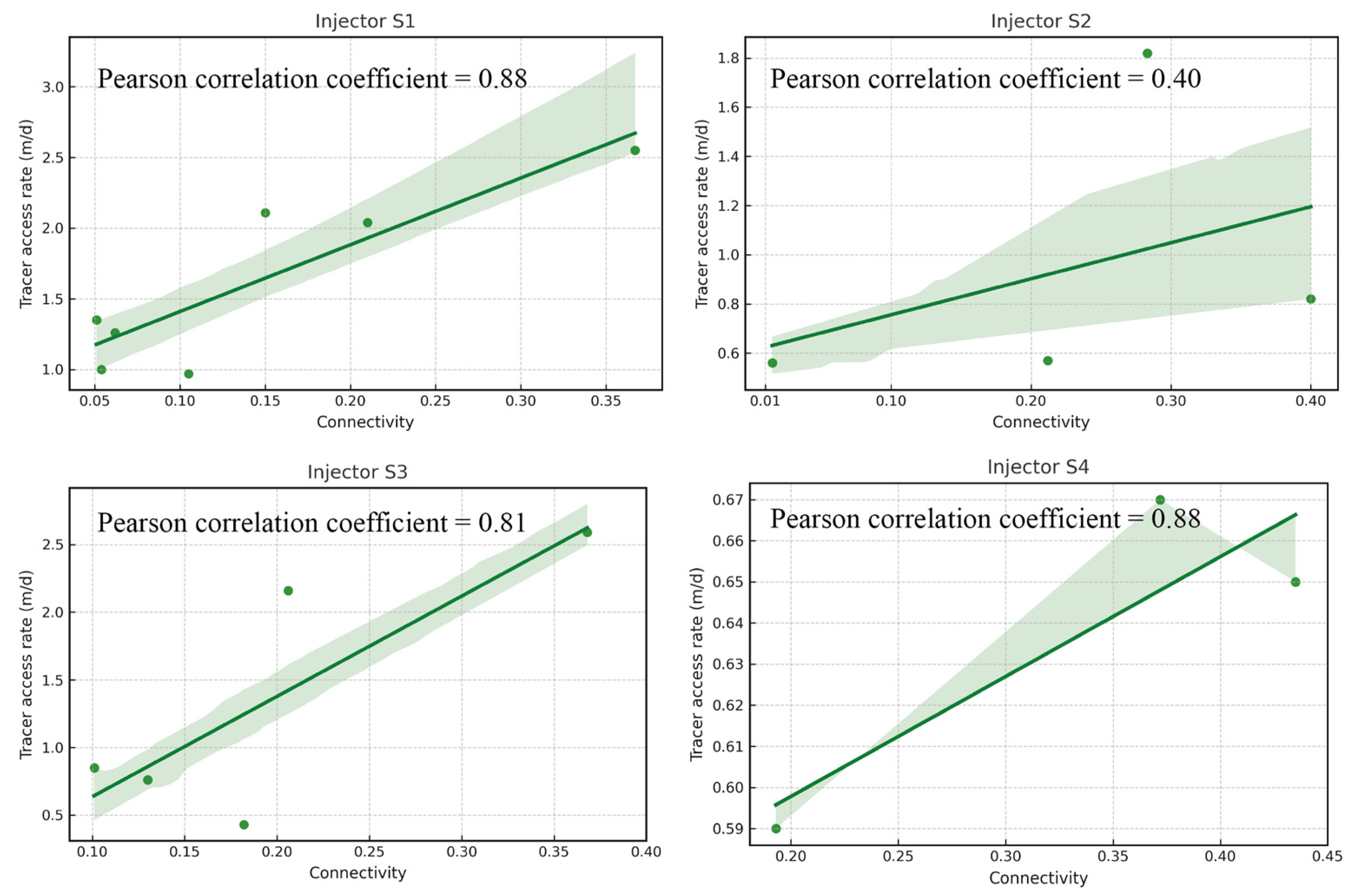
- The inter-well connectivity calculated by the algorithm demonstrated a consistent correspondence with the tracer access rate from the tracer test. The Pearson correlation coefficients for the results of the four injectors ranged from 0.4 to 0.88, indicating a moderate to strong positive correlation. Notably, three of the injectors exhibited Pearson correlation coefficients above 0.8, demonstrating a strong positive correlation.
- (4)
- The algorithm demonstrates stable performance when processing production history data for water flooding and continuous CO2 flooding. However, it faces limitations when handling production data under water-gas alternating injection patterns. This is primarily due to the presence of three-phase flow involving oil, gas, and water in the production rates. After gas breakthrough in the producers, gas production rate significantly increases, leading to itself and oil production rates being of different magnitudes. Consequently, fluctuations in oil production are masked, resulting in the inability to generate reliable results consistently.
Author Contributions
Funding
Data Availability Statement
Conflicts of Interest
References
- Liao, M.; Liao, C.; Chen, X. Application of dynamic and static analyses in inter-well connectivity characterization. Spec. Oil Gas Reserv. 2020, 27, 131–136. [Google Scholar]
- Liu, W.; Liu, W.D.; Gu, J. A Machine Learning Method to infer inter-well connectivity using bottom-hole pressure data. J. Energy Resour. Technol. 2020, 142, 103007. [Google Scholar] [CrossRef]
- Ma, C.; Zhang, H.; Yao, W.; Chen, K.; Zhang, Q. Research and Application of lnterwell Connectivity Based on System ldentification Method in Offshore Oilfields. Liaoning Chem. Ind. 2021, 50, 1654–1657. [Google Scholar] [CrossRef]
- Singh, N.P. Permeability prediction from wireline logging and core data: A case study from Assam-Arakan basin. J. Pet. Explor. Prod. Technol. 2019, 9, 297–305. [Google Scholar] [CrossRef]
- Liang, J.S.; Zheng, W.; Yuan, Z.B. Well Group Connectivity Relations Discriminate Based on CART Algorithm. Appl. Mech. Mater. 2014, 513, 1252–1255. [Google Scholar] [CrossRef]
- Zhang, H.; Zhou, X.; Wang, A. Log Evaluation Method for Fractured-Vuggy Reservoir in the Dengying Formation of the Anyue Block, Sichuan Basin. Well Logging Technol. 2018, 42, 91–97. [Google Scholar] [CrossRef]
- Mirzayev, M.; Riazi, N.; Cronkwright, D.; Jensen, J.L.; Pedersen, P.K. Determining well-to-well connectivity using a modified capacitance model, seismic, and geology for a Bakken Waterflood. J. Pet. Sci. Eng. 2017, 152, 611–627. [Google Scholar] [CrossRef]
- Yin, Z.; MacBeth, C.; Chassagne, R.; Vazquez, O. Evaluation of inter-well connectivity using well fluctuations and 4D seismic data. J. Pet. Sci. Eng. 2016, 145, 533–547. [Google Scholar] [CrossRef]
- Jiang, X.; Qu, Y.; Wu, J.; Zhao, Y. Research Progress of Superior Reservoir Channels and Interwell Connectivity. Liaoning Chem. Ind. 2022, 51, 261–265. [Google Scholar] [CrossRef]
- Lu, L.; Yang, Z.; Sun, H. Analysis of gas well connectivity based on dynamic and static data: A case study from the volcanic gas reservoirs in the Kelameili Gas Field. Nat. Gas Ind. 2012, 32, 58–61. [Google Scholar]
- Jansen, F.; Kelkar, M. Application of wavelets to production data in describing inter-well relationships. In Proceedings of the SPE Annual Technical Conference and Exhibition, San Antonio, TX, USA, 5–8 October 1997. Paper Number: SPE-38876-MS. [Google Scholar]
- Wen, T.; Zhai, X.; Matringe, S. Inter-well Connectivity in Waterfloods-Modelling, Uncertainty Quantification, and Production Optimization. In Proceedings of the ECMOR XV-15th European Conference on the Mathematics of Oil Recovery, Amsterdam, The Netherlands, 29 August–1 September 2016. [Google Scholar]
- Kukar, M.; Kononenko, I. Reliable classifications with machine learning. In Proceedings of the Machine Learning: ECML 2002: 13th European Conference on Machine Learning, Helsinki, Finland, 19–23 August 2002; Proceedings 13. pp. 219–231. [Google Scholar]
- Heffer, K.J.; Fox, R.J.; McGill, C.A.; Koutsabeloulis, N.C. Novel Techniques Show Links between Reservoir Flow Directionality, Earth Stress, Fault Structure and Geomechanical Changes in Mature Waterfloods. SPE J. 1997, 2, 91–98. [Google Scholar] [CrossRef]
- Fedenczuk, L.; Hoffmann, K. Surveying and analyzing injection responses for patterns with horizontal wells. In Proceedings of the SPE/CIM International Conference on Horizontal Well Technology, Calgary, AB, Canada, 1–4 November 1998. [Google Scholar]
- Soeriawinata, T.; Kelkar, M. Reservoir management using production data. In Proceedings of the SPE Oklahoma City Oil and Gas Symposium/Production and Operations Symposium, Oklahoma City, OK, USA, 28–31 March 1999. [Google Scholar]
- Albertoni, A.; Lake, L.W. Inferring interwell connectivity only from well-rate fluctuations in waterfloods. SPE Reserv. Eval. Eng. 2003, 6, 6–16. [Google Scholar] [CrossRef]
- Anh, D.V.; Tiab, D. Inferring interwell connectivity in a reservoir from bottomhole pressure fluctuations of hydraulically fractured vertical wells, horizontal wells, and mixed wellbore conditions. Petrovietnam J. 2020, 10, 20–40. [Google Scholar]
- Wang, J.; Shen, H.; Qiu, Y.; Wang, B.; Zhang, P.; Mo, L.; Chen, G. Feasibility Analysis of Interwell Dynamic Connectivity InversionModel Based on Multivariate Linear RegressionTaking Chang-6 Reservoir in Wuliwan Area 1 of Jing’an Oilfield as an Example. Unconventonal Oil Gas 2019, 6, 57–62+34. [Google Scholar]
- Yousef, A.A.; Gentil, P.; Jensen, J.L.; Lake, L.W. A capacitance model to infer interwell connectivity from production-and injection-rate fluctuations. SPE Reserv. Eval. Eng. 2006, 9, 630–646. [Google Scholar] [CrossRef]
- Kaviani, D.; Jensen, J.L.; Lake, L.W. Estimation of interwell connectivity in the case of unmeasured fluctuating bottomhole pressures. J. Pet. Sci. Eng. 2012, 90, 79–95. [Google Scholar] [CrossRef]
- Mirzayev, M.; Jensen, J.L. Measuring interwell communication using the capacitance model in tight reservoirs. In Proceedings of the SPE Western Regional Meeting, Anchorage, AK, USA, 23–26 May 2016. [Google Scholar]
- Yu, H.; Wang, H.; Lian, Z. An assessment of seal ability of tubing threaded connections: A hybrid empirical-numerical method. J. Energy Resour. Technol. 2023, 145, 052902. [Google Scholar] [CrossRef]
- An, F.; Wang, J.; Liu, R. Road Traffic Sign Recognition Algorithm Based on Cascade Attention-Modulation Fusion Mechanism. IEEE Trans. Intell. Transp. Syst. 2024. [Google Scholar] [CrossRef]
- Mahesh, B. Machine learning algorithms-a review. Int. J. Sci. Res. (IJSR) 2020, 9, 381–386. [Google Scholar] [CrossRef]
- Dai, T.; Fang, C.; Liu, T.; Zheng, S.; Lei, G.; Jiang, G. Waste glass powder as a high temperature stabilizer in blended oil well cement pastes: Hydration, microstructure and mechanical properties. Constr. Build. Mater. 2024, 439, 137359. [Google Scholar] [CrossRef]
- Zhu, Y.; Dai, H.; Yuan, S. The competition between heterotrophic denitrification and DNRA pathways in hyporheic zone and its impact on the fate of nitrate. J. Hydrol. 2023, 626, 130175. [Google Scholar] [CrossRef]
- Li, J.; Pang, Z.; Liu, Y.; Hu, S.; Jiang, W.; Tian, L.; Yang, G.; Jiang, Y.; Jiao, X.; Tian, J. Changes in groundwater dynamics and geochemical evolution induced by drainage reorganization: Evidence from 81Kr and 36Cl dating of geothermal water in the Weihe Basin of China. Earth Planet. Sci. Lett. 2023, 623, 118425. [Google Scholar] [CrossRef]
- Liu, W.; Liu, W.D.; Gu, J. Reservoir inter-well connectivity analysis based on a data driven method. In Proceedings of the Abu Dhabi International Petroleum Exhibition and Conference, Abu Dhabi, United Arab Emirates, 11–14 November 2019. [Google Scholar]
- Jiang, Y.; Zhang, H.; Zhang, K.; Wang, J.; Han, J.; Cui, S.; Zhang, L.; Zhao, H.; Liu, P.; Song, H. Waterflooding Interwell Connectivity Characterization and Productivity Forecast with Physical Knowledge Fusion and Model Structure Transfer. Water 2023, 15, 218. [Google Scholar] [CrossRef]
- Alanne, K.; Sierla, S. An overview of machine learning applications for smart buildings. Sustain. Cities Soc. 2022, 76, 103445. [Google Scholar] [CrossRef]
- Huang, S.; Jia, A.; Zhang, X.; Wang, C.; Shi, X.; Xu, T. Application of Inter-Well Connectivity Analysis with a Data-Driven Method in the SAGD Development of Heavy Oil Reservoirs. Energies 2023, 16, 3134. [Google Scholar] [CrossRef]
- Sinha, U.; Gautam, S.; Dindoruk, B.; Abdulwarith, A. Machine Learning-Enhanced Forecasting for Efficient Water-Flooded Reservoir Management. In Proceedings of the SPE Improved Oil Recovery Conference, Tulsa, OK, USA, 22–25 April 2024. [Google Scholar]
- Yu, J.; Jahandideh, A.; Hakim-Elahi, S.; Jafarpour, B. Sparse neural networks for inference of interwell connectivity and production prediction. SPE J. 2021, 26, 4067–4088. [Google Scholar] [CrossRef]
- Li, Y.; Suzuki, S.; Horne, R. Well Connectivity Analysis with Deep Learning. In Proceedings of the SPE Annual Technical Conference and Exhibition, Dubai, United Arab Emirates, 21–23 September 2021. [Google Scholar]
- Bentur, A.; Igarashi, S.-I.; Kovler, K. Prevention of autogenous shrinkage in high-strength concrete by internal curing using wet lightweight aggregates. Cem. Concr. Res. 2001, 31, 1587–1591. [Google Scholar] [CrossRef]
- Justs, J.; Wyrzykowski, M.; Bajare, D.; Lura, P. Internal curing by superabsorbent polymers in ultra-high performance concrete. Cem. Concr. Res. 2015, 76, 82–90. [Google Scholar] [CrossRef]
- Schröfl, C.; Mechtcherine, V.; Gorges, M. Relation between the molecular structure and the efficiency of superabsorbent polymers (SAP) as concrete admixture to mitigate autogenous shrinkage. Cem. Concr. Res. 2012, 42, 865–873. [Google Scholar] [CrossRef]
- Li, H.; Deng, J.; Feng, Y.; Dong, B.; Ding, J.; Cao, Z. Research status and development trend of oilfield tracer technology. Appl. Chem. Ind. 2023, 52, 3163–3168+3174. [Google Scholar] [CrossRef]
- Pedregosa, F.; Varoquaux, G.; Gramfort, A.; Michel, V.; Thirion, B.; Grisel, O.; Blondel, M.; Prettenhofer, P.; Weiss, R.; Dubourg, V. Scikit-learn: Machine learning in Python. J. Mach. Learn. Res. 2011, 12, 2825–2830. [Google Scholar]
- Friedman, J.; Hastie, T.; Tibshirani, R. Sparse inverse covariance estimation with the graphical lasso. Biostatistics 2008, 9, 432–441. [Google Scholar] [CrossRef]
- Frey, B.J.; Dueck, D. Clustering by passing messages between data points. Science 2007, 315, 972–976. [Google Scholar] [CrossRef] [PubMed]
- Zhang, L.; Liao, X.; Shen, C.; Dong, P.; Ou, Y.; Tao, R.; Wang, X. A New Method for Automatic Identification of Inter-Well Connectivity in Heterogeneous Reservoirs Based on Affinity Propagation Unsupervised Learning. In Proceedings of the SPE Conference at Oman Petroleum & Energy Show, Muscat, Oman, 22–24 April 2024. [Google Scholar]
- Dallakyan, A. graphiclasso: Graphical lasso for learning sparse inverse-covariance matrices. Stata J. 2022, 22, 625–642. [Google Scholar] [CrossRef]
- MacQueen, J. Some methods for classification and analysis of multivariate observations. Berkeley Symp. Math. Stat. Probab. 1967, 5.1, 281–297. [Google Scholar]
- Murtagh, F.; Contreras, P. Algorithms for hierarchical clustering: An overview. Wiley Interdiscip. Rev. Data Min. Knowl. Discov. 2012, 2, 86–97. [Google Scholar] [CrossRef]
- Liu, P.; Zhou, D.; Wu, N. VDBSCAN: Varied density based spatial clustering of applications with noise. In Proceedings of the 2007 International Conference on Service Systems and Service Management, Chengdu, China, 9–11 June 2007; pp. 1–4. [Google Scholar]
- Fiedler, M. Algebraic connectivity of graphs. Czechoslov. Math. J. 1973, 23, 298–305. [Google Scholar] [CrossRef]
- Bodenhofer, U.; Kothmeier, A.; Hochreiter, S. APCluster: An R package for affinity propagation clustering. Bioinformatics 2011, 27, 2463–2464. [Google Scholar] [CrossRef]
- Lee Rodgers, J.; Nicewander, W.A. Thirteen ways to look at the correlation coefficient. Am. Stat. 1988, 42, 59–66. [Google Scholar] [CrossRef]


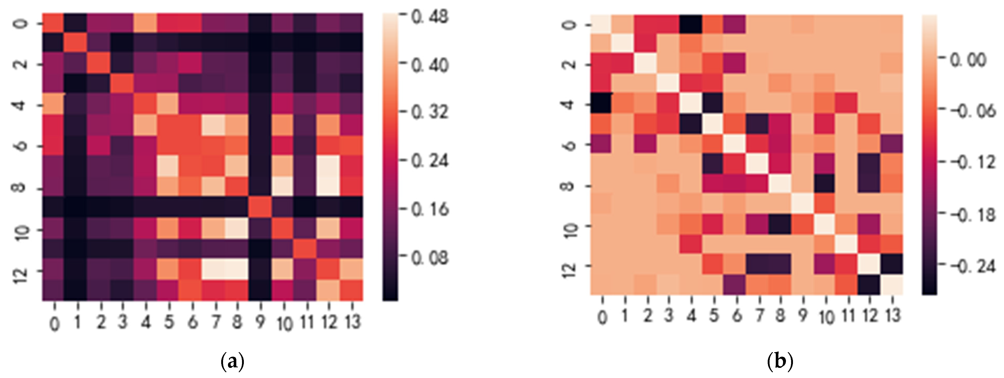
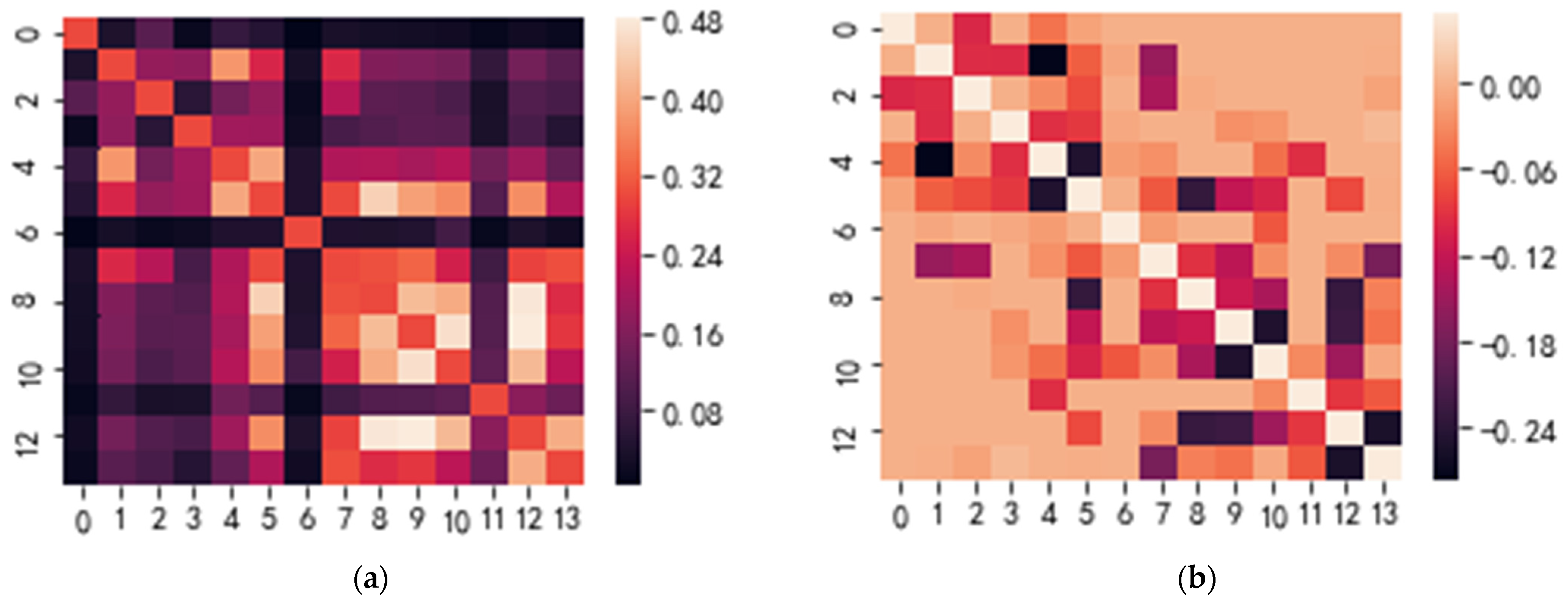
| B2 | B3 | B7 | B8 | B10 | B12 | B13 | B17 | B22 | B23Z | B25 | B30Y | B31 | B38 | |
|---|---|---|---|---|---|---|---|---|---|---|---|---|---|---|
| B2 | −0.214 | −0.345 | −0.214 | −0.268 | 0.204 1 | −0.344 | −0.204 | −0.514 | −0.519 | −0.345 | −0.529 | −0.381 | −0.268 | −0.530 |
| B3 | −0.308 | 0.032 | −0.033 | −0.267 | −0.054 | −0.303 | −0.227 | −0.450 | −0.453 | −0.177 | −0.470 | −0.223 | −0.177 | −0.443 |
| B7 | −0.213 | −0.033 | −0.018 | −0.252 | 0.018 | −0.228 | −0.092 | −0.308 | −0.307 | −0.192 | −0.344 | −0.220 | −0.040 | −0.316 |
| B8 | −0.231 | −0.267 | −0.252 | −0.068 | 0.068 | −0.231 | −0.249 | −0.426 | −0.353 | −0.173 | −0.374 | −0.254 | −0.162 | −0.508 |
| B10 | −0.278 | −0.370 | −0.316 | −0.316 | 0.276 | −0.274 | −0.324 | −0.544 | −0.536 | −0.399 | −0.517 | −0.346 | −0.334 | −0.629 |
| B12 | −0.348 | −0.344 | −0.234 | −0.273 | 0.028 | −0.228 | −0.188 | −0.283 | −0.281 | −0.406 | −0.321 | −0.355 | −0.028 | −0.449 |
| B13 | −0.242 | −0.302 | −0.092 | −0.324 | −0.083 | −0.228 | −0.092 | −0.283 | −0.275 | −0.250 | −0.334 | −0.319 | 0.083 | −0.266 |
| B17 | −0.542 | −0.516 | −0.374 | −0.492 | −0.293 | −0.255 | −0.260 | −0.283 | −0.328 | −0.495 | −0.364 | −0.436 | 0.254 | −0.472 |
| B22 | −0.562 | −0.533 | −0.387 | −0.433 | −0.300 | −0.320 | −0.247 | −0.343 | −0.275 | −0.441 | −0.308 | −0.436 | 0.247 | −0.466 |
| B23Z | −0.308 | −0.177 | −0.192 | −0.173 | −0.083 | −0.365 | −0.175 | −0.430 | −0.361 | 0.083 | −0.331 | −0.226 | −0.163 | −0.443 |
| B25 | −0.492 | −0.470 | −0.344 | −0.374 | −0.201 | −0.280 | −0.259 | −0.299 | −0.275 | −0.331 | −0.293 | −0.345 | 0.201 | −0.460 |
| B30Y | −0.344 | −0.223 | −0.220 | −0.254 | −0.030 | −0.314 | −0.244 | −0.371 | −0.355 | −0.226 | −0.345 | −0.046 | 0.030 | −0.303 |
| B31 | −1.220 | −1.166 | −1.029 | −1.150 | −1.007 | −0.975 | −0.914 | −0.923 | −0.908 | −1.152 | −0.989 | −0.989 | 0.921 | −0.977 |
| B38 | −0.505 | −0.455 | −0.328 | −0.520 | −0.325 | −0.420 | −0.191 | −0.419 | −0.397 | −0.455 | −0.472 | −0.315 | 0.191 | −0.266 |
| Cluster Group | Well Number | Cluster Center |
|---|---|---|
| 1 | B3 | B3 |
| 2 | B2, B7, B8, B10, B12 | B10 |
| 3 | B23Z | B23Z |
| 4 | B13, B17, B22, B25, B30Y, B31, B38 | B31 |
| Well Number | Responsibility | Connectivity | Time of Tracer Arrival d | Well Distance m | Tracer Access Rate m/d | Tracer Peak Concentration ppb | Tracer Peak Width d | Tracer Current Concentration ppb |
|---|---|---|---|---|---|---|---|---|
| S1 | −0.16806 | - | - | - | - | - | - | - |
| B2 | −0.01502 | 0.367 | 1302 (3.6 years) | 3314 | 2.55 | 200 | 27 | 0.91 |
| B3 | −0.23451 | - | - | - | - | - | - | - |
| B7 | −0.21688 | - | - | - | - | - | - | - |
| B8 | −0.24073 | - | - | - | - | - | - | - |
| B10 | −0.05243 | 0.210 | 1610 (4.4 years) | 3280 | 2.04 | 80 | 38 | 0.81 |
| B12 | −0.10518 | 0.062 | 2603 (7.1 years) | 3275 | 1.26 | 44 | 116 | 7.75 |
| B13 | −0.21440 | - | - | |||||
| B17 | −0.27691 | - | 2781 (7.6 years) | 3836 | 1.38 | 33 | 57 | 1.58 |
| B22 | −0.22857 | - | - | - | - | - | - | - |
| B23Z | −0.07011 | 0.150 | 1724 (4.7 years) | 3639 | 2.11 | 25 | 66 | 16 |
| B25 | −0.11096 | 0.051 | 2716 (7.4 years) | 3679 | 1.35 | 30 | 587 | 1.73 |
| B30Y | −0.08618 | 0.105 | 2520 (6.9 years) | 2454 | 0.97 | 27 | 72 | 0.36 |
| B31 | −1.38504 | - | - | - | - | - | - | - |
| B38 | −0.10935 | 0.054 | 3007 (8.2 years) | 2994 | 1.00 | 23 | 109 | 1.66 |
| Well Number | Responsibility | Connectivity | Time of Tracer Arrival d | Well Distance m | Tracer Access Rate m/d | Tracer Peak Concentration ppb | Tracer Peak Width d | Tracer Current Concentration ppb |
|---|---|---|---|---|---|---|---|---|
| S2 | −0.26029 | - | - | - | - | - | - | - |
| B2 | −0.22552 | 0.003 | - | - | - | - | - | - |
| B3 | −0.39248 | - | - | - | - | - | - | |
| B7 | −0.08248 | 0.400 | 1895 (5.2 years) | 1558 | 0.82 | 11 | 1144 | 2.88 |
| B8 | −0.15862 | 0.075 | - | - | - | - | - | - |
| B10 | −0.21212 | 0.008 | - | - | - | - | - | - |
| B12 | −0.20017 | 0.015 | 4802 (13.2 years) | 2688 | 0.56 | 6.61 | 59 | 0.31 |
| B13 | −0.10191 | 0.283 | 1288 (3.5 years) | 2341 | 1.82 | 41 | 76 | 1.46 |
| B17 | −0.32331 | - | - | - | - | - | - | - |
| B22 | −0.33142 | - | - | - | - | - | - | - |
| B23Z | −0.42384 | - | - | - | - | - | - | - |
| B25 | −0.30059 | - | - | - | - | - | - | - |
| B30Y | −0.11645 | 0.212 | 3506 (9.6 years) | 2006 | 0.57 | 5.6 | 79 | 0.66 |
| B31 | −0.76099 | - | - | - | - | - | - | - |
| B38 | −0.21986 | 0.005 | - | - | - | - | - | - |
| Well Number | Responsibility | Connectivity | Time of Tracer Arrival d | Well Distance m | Tracer Access Rate m/d | Tracer Peak Concentration ppb | Tracer Peak Width d | Tracer Current Concentration ppb |
|---|---|---|---|---|---|---|---|---|
| S3 | −0.12755 | - | - | - | - | - | - | - |
| B2 | −0.07960 | 0.368 | 1118 (3.1 years) | 2898 | 2.59 | 11 | 44 | 4.3 |
| B3 | −0.19022 | - | - | - | - | - | - | - |
| B7 | −0.09385 | 0.182 | 5533 (15.2 years) | 2378 | 0.43 | 4.03 | 195 | 4.03 |
| B8 | −0.11838 | 0.013 | - | - | - | - | - | - |
| B10 | −0.09902 | 0.130 | 3779 (10.4 years) | 2878 | 0.76 | 12 | 24 | 2.33 |
| B12 | −0.27936 | - | - | - | - | - | - | - |
| B13 | −0.09169 | 0.206 | 1520 (4.2 years) | 3288 | 2.16 | 330 | 23 | 0.22 |
| B17 | −0.26696 | - | 5078 (13.9 years) | 3415 | 0.67 | 10.85 | 144 | 10.85 |
| B22 | −0.27268 | - | - | - | - | - | - | - |
| B23Z | −0.12762 | - | - | - | - | - | - | - |
| B25 | −0.10245 | 0.101 | 3880 (10.6 years) | 3291 | 0.85 | 20.79 | 181 | 3.42 |
| B30Y | −0.24667 | - | - | - | - | - | - | - |
| B31 | −0.32515 | - | - | - | - | - | - | - |
| B38 | −0.23590 | - | - | - | - | - | - | - |
| Well Number | Responsibility | Connectivity | Time of Tracer Arrival d | Well Distance m | Tracer Access Rate m/d | Tracer Peak Concentration ppb | Tracer Peak Width d | Tracer Current Concentration ppb |
|---|---|---|---|---|---|---|---|---|
| S4 | −0.09306 | - | - | - | - | - | - | - |
| B2 | −0.15851 | - | - | - | - | - | - | - |
| B3 | −0.13416 | - | - | - | - | - | - | - |
| B7 | −0.11343 | - | - | - | - | - | - | - |
| B8 | −0.12233 | - | - | - | - | - | - | - |
| B10 | −0.11047 | 0.435 | 4871 (13.3 years) | 3184 | 0.65 | 16.44 | 60 | 0.13 |
| B12 | −0.04682 | 0.372 | 4871 (13.3 years) | 3244 | 0.67 | 6.69 | 53 | 2.45 |
| B13 | −0.05027 | - | - | - | - | - | - | - |
| B17 | −0.12878 | - | - | - | - | - | - | - |
| B22 | −0.24865 | - | - | - | - | - | - | - |
| B23Z | −0.23282 | - | - | - | - | - | - | - |
| B25 | −0.11565 | - | - | - | - | - | - | - |
| B30Y | −0.22640 | 0.193 | 4165 (11.4 years) | 2443 | 0.59 | 6.21 | 675 | 4.29 |
| B31 | −0.06222 | - | - | - | - | - | - | - |
| B38 | −0.55428 | - | - | - | - | - | - | - |
Disclaimer/Publisher’s Note: The statements, opinions and data contained in all publications are solely those of the individual author(s) and contributor(s) and not of MDPI and/or the editor(s). MDPI and/or the editor(s) disclaim responsibility for any injury to people or property resulting from any ideas, methods, instructions or products referred to in the content. |
© 2024 by the authors. Licensee MDPI, Basel, Switzerland. This article is an open access article distributed under the terms and conditions of the Creative Commons Attribution (CC BY) license (https://creativecommons.org/licenses/by/4.0/).
Share and Cite
Zhang, L.; Liao, X.; Dong, P.; Hou, S.; Li, B.; Chen, Z. An Efficient Method for Identifying Inter-Well Connectivity Using AP Clustering and Graphical Lasso: Validation with Tracer Test Results. Processes 2024, 12, 2143. https://doi.org/10.3390/pr12102143
Zhang L, Liao X, Dong P, Hou S, Li B, Chen Z. An Efficient Method for Identifying Inter-Well Connectivity Using AP Clustering and Graphical Lasso: Validation with Tracer Test Results. Processes. 2024; 12(10):2143. https://doi.org/10.3390/pr12102143
Chicago/Turabian StyleZhang, Lingfeng, Xinwei Liao, Peng Dong, Shanze Hou, Boying Li, and Zhiming Chen. 2024. "An Efficient Method for Identifying Inter-Well Connectivity Using AP Clustering and Graphical Lasso: Validation with Tracer Test Results" Processes 12, no. 10: 2143. https://doi.org/10.3390/pr12102143
APA StyleZhang, L., Liao, X., Dong, P., Hou, S., Li, B., & Chen, Z. (2024). An Efficient Method for Identifying Inter-Well Connectivity Using AP Clustering and Graphical Lasso: Validation with Tracer Test Results. Processes, 12(10), 2143. https://doi.org/10.3390/pr12102143