Abstract
Considering energy conversion efficiency, pollution emissions, and economic benefits, combining biomass with fossil fuels in power generation facilities is a viable approach to address prevailing energy deficits and environmental challenges. This research aimed to investigate the thermodynamic and exergoeconomic performance of a novel power and cooling cogeneration system based on a natural gas–biomass dual fuel gas turbine (DFGT). In this system, a steam Rankine cycle (SRC), a single-effect absorption chiller (SEAC), and an organic Rankine cycle (ORC) are employed as bottoming cycles for the waste heat cascade utilization of the DFGT. The effects of main operating parameters on the performance criteria are examined, and multi-objective optimization is accomplished with a genetic algorithm using exergy efficiency and the sum unit cost of the product (SUCP) as the objective functions. The results demonstrate the higher energy utilization efficiency of the proposed system with the thermal and exergy efficiencies of 75.69% and 41.76%, respectively, while the SUCP is 13.37 $/GJ. The exergy analysis reveals that the combustion chamber takes the largest proportion of the exergy destruction rate. The parametric analysis shows that the thermal and exergy efficiencies, as well as the SUCP, rise with the increase in the gas turbine inlet temperature or with the decrease in the preheated air temperature. Higher exergy efficiency and lower SUCP could be obtained by increasing the SRC turbine inlet pressure or decreasing the SRC condensation temperature. Finally, optimization results indicate that the system with an optimum solution yields 0.3% higher exergy efficiency and 2.8% lower SUCP compared with the base case.
1. Introduction
Energy consumption has been on a long-term upward trend, paralleling the rapid advancement of societal and economic sectors. As the primary energy source, fossil fuels satisfy approximately 80% of the world’s total energy demand [1]. The global CO2 emissions from fossil fuel combustion have increased by 2.5% annually on average in the last decade [2]. The large-scale energy consumption of fossil fuels all over the globe is responsible for the serious environmental problems, like global warming and air pollution. Additionally, the energy crisis has catalyzed a shift towards optimizing the use of non-renewable energy sources and advancing the development of renewable energy alternatives.
Biomass, characterized as a renewable energy source, produces minimal-to-zero carbon dioxide emissions and predominantly originates from sources, including forests, agricultural residues, municipal solid waste, sewage, and industrial by-products [3]. In general, biomass energy can help mitigate the environmental problems and improve the energy self-sufficiency of nations that rely on imported fossil fuels. Numerous contemporary energy strategies are in place to facilitate the adoption of biofuels. According to the survey of IEA (International Energy Agency), in China, biofuels contribute around 1.90% of the total energy supply for electricity generation [4].
There are still many problems impeding the widespread use of biomass for power generation. The energy conversion efficiencies of biomass-based power plants are relatively low, typically ranging from 15% for small plants to 30% for large ones, in comparison with the most efficient energy conversion plants, such as the natural gas combined cycles [5]. Furthermore, the use of biomass or biomass-derived fuels in the power plants has some limitations regarding fuel flexibility and system reliability, as well as economic feasibility. The investment and operational costs related to biomass processing and transport facilities are expensive for large-scale utilization [6]. To overcome these drawbacks, researchers have integrated biomass into conventional fossil fuel power generation systems, in which biomass serves as a supplementary fuel [7,8]. In particular, for a gas turbine (GT) cycle, biomass or biomass-derived fuel burns at the end of the GT cycle in a supplementary firing chamber, capitalizing on the surplus oxygen present in high-temperature combustion gases. This method not only maintains system functionality but also curtails the consumption of natural gas and CO2 emissions, further augmenting system efficiency through the integration of bottoming heat recovery systems [9,10]. Moreover, the mechanism of biomass post-combustion provides the possibility of using commercially available components or directly combine with the commercial micro gas turbine (MGT) without major modifications [11].
In recent years, various solutions for coupling biomass with natural gas in the GT-based power plants have been proposed. Riccio et al. [11] matched an externally biomass-fired cycle with a commercial MGT and theoretically evaluated the thermodynamic performance of the plant. They found that the system could achieve a net electric efficiency of 21.8% when the biomass accounted for 70% of the total energy input. Gnanapragasam et al. [12] investigated a GT-based combined cycle with the external combustion of biomass in a supplementary firing chamber. They found that the reduction in CO2 emissions and natural gas could reach 20 g/kWh and 1.5 kg/s, respectively. Pantaleo et al. [13] analyzed various operational approaches for a small-scale combined heat and power system using a natural gas-biomass DFGT. Their findings revealed that thermal and electrical conversion efficiencies fluctuate between 46 and 38% and 30 and 19%, respectively, with system efficacy showing an inverse relationship with the rate of biomass input. Furthermore, their research deduced that optimal investment returns are attainable when the biomass input constitutes 70%, taking into account Italy’s biomass electricity incentives, investment expenditures, and energy conversion efficiency [6]. Barzegaravval et al. [14] studied the impact of the biogas composition on both the exergetic and economic aspects of the GT cycle’s performance. They reported that the cost of generated electricity varies from 0.05 $/kWh to 0.18 $/kWh when the fuel price increases from 3 $/GJ to 14 $/GJ. Also, the idea of a biomass and natural gas co-fired combined cycle by employing the SRC as a bottoming cycle for power generation has been proposed and extensively studied [15,16,17]. Soltani et al. [18] examined a biomass-integrated fired combined cycle (BIFCC) from the viewpoints of energy and exergy. Their observations noted that, across the explored range of operational parameters, the energy efficiency varied between 46.48% and 53.16%.
Another key factor in improving the efficiency of a GT-based combined cycle is the selection of proper energy conversion techniques based on the heat source characteristics to reduce the irreversible losses. Recently, many researchers combined various waste heat recovery systems with GT cycles using biofuels for multi-generation. Gholizadeh et al. [19] conducted an exergoeconomic evaluation of a bi-evaporator power and cooling cogeneration system with a topping biogas-powered GT cycle. They reported achieving overall thermal and exergy efficiencies of 62.69% and 38.75%, respectively, with a total unit cost of 7.75 $/GJ. Yilmaz et al. [20] evaluated a biomass-solar multi-generation system from the techno-economic perspective. In the study, the GT cycle was driven by biogas, with its waste heat being utilized for a Kalina cycle, an SEAC, and a heat pump cycle (HPC). The findings revealed overall energy and exergy efficiencies of 63.84% and 59.26%, respectively. Zhang et al. [21] assessed a multi-generation system consisting of a biogas-fueled GT, a compressed air energy storage (CAES), and a ground source heat pump (GSHP) from thermodynamic and economic viewpoints. They defined the round trip efficiency and exergy efficiency to evaluate the system operation characteristics, and their values were calculated to be 90.06% and 31.52%, respectively. Asgari et al. [22] thermodynamically evaluated a GT-based trigeneration system fed by both natural gas and syngas derived from municipal solid waste. In this system, the waste heat from the GT cycle and the gasification unit is used as the heat source of two heat recovery steam generators (HRSGs), while an SEAC and a heating unit are driven by the steam. The outcomes showed that the annual energy utilization factor and exergy efficiency of the overall system are 71.25% and 30.79%, respectively. Zoghi et al. [23] undertook exergoeconomic and environmental examinations of a biomass-solar multi-generation system. This system utilizes the waste heat from a GT cycle as a heat source for an SRC, a domestic water heater, and a LiCl-H2O SEAC. Their findings indicated that, in the base scenario, the overall exergy efficiency reached 43.11%, marking an increase of 9.04% over the exergy efficiency of a standalone GT cycle.
Previous research findings have demonstrated that combining biomass energy with waste heat recovery systems in the GT cycle stands as a highly effective approach to improve energy conversion efficiency and meet the various energy demands of users. Steam Rankine cycles, widely recognized as a leading technology for waste heat recovery, are typically employed to recover medium- or high-temperature waste heat due to the advantages of the working fluid with a high decomposition temperature, non-toxicity, environmentally friendliness, and cost-effectiveness [24]. However, in most studied SRCs, a considerable volume of thermal energy is released into the atmosphere, remaining unutilized, throughout their condensation processes. One effective way to recover the condensation latent heat is using LiBr/H2O absorption refrigeration systems, which are available to utilize the heat source with a temperature ranging from 50 °C to 200 °C [25]. Liang et al. [24,26] investigated a cogeneration system by coupling an SRC and an SEAC to recover the waste heat of a marine engine. Their research indicated that the exergy efficiency of the cogeneration system increases by 84% compared with the basic SRC under conditions of a condensation temperature at 323 K and superheat at 100 K. Sahoo et al. [27] analyzed a solar-biomass multi-generation system, utilizing the residual heat from the SRC to power an SEAC. Their study demonstrated that the system’s energy and exergy efficiencies could achieve 49.85% and 20.94%, respectively. Ahmadi et al. [28] performed an exergo-environmental analysis of a GT-based trigeneration system integrated with an SRC and a steam-driven SEAC. They reported the thermal and exergy efficiencies of 75.5% and 47.5%, respectively. Anvari et al. [29] applied advanced exergetic and exergoeconomic concepts to assess a GT-based trigeneration system using a dual pressure HRSG and a steam-driven SEAC as bottoming cycles. They identified that nearly 29% of the exergy destruction in the cycle and the corresponding cost rates are endogenously avoidable. Nondy et al. [30] thermodynamically evaluated four GT-based cogeneration systems, in which the SEAC is driven by the heat from the SRC or exhaust gas. They concluded that the system with two SEACs driven, respectively, by steam and exhaust heat is the most appropriate from the viewpoints of energy and exergy.
A comprehensive examination of the aforementioned research suggests that the natural gas combined with biomass energy is a practicable scheme for GT-based multi-generation systems from the technical and economic aspects, which can help to reduce the fossil fuel consumption and mitigate the environmental impact. The literature review also reveals that the coupling of SRC and SEAC contributes to further improving the energy utilization efficiency. Based on recent studies [15,18], some of the researchers have already conducted the thermodynamic and exergoeconomic analyses of a biomass-integrated co-fired combined cycle (BICFCC), in which the waste heat of the DFGT cycle is only converted into power by the SRC or ORC.
To the best of the authors’ knowledge, there have been few studies on BICFCC to date. The novelty of this work lies in expanding the application of BICFCC to power and cooling cogeneration systems through the integration of high-efficiency subsystems, including an SRC, an SEAC, and an ORC. These subsystems are not typically utilized in BICFCC configurations, highlighting the unique contribution of this research. The exhaust gas flows into the SRC and ORC in sequence for power, while the condensation heat of the SRC is converted into the cooling capacity by the SEAC. Compared with the BICFCC, the cogeneration system in this work could exploit the waste heat sufficiently to achieve the higher energy utilization efficiency and satisfy different kinds of energy demands. The primary purposes of this work can be considered as follows:
- (1)
- A novel DFGT-based cogeneration system is proposed, and detailed thermodynamic and economic models are developed for simulating the system’s performance.
- (2)
- In-depth parametric analysis is carried out to assess the impact of crucial operation parameters on the performance criteria.
- (3)
- Multi-objective optimization is performed to ascertain the most favorable operating conditions for the proposed system.
2. System Description
Figure 1 illustrates the schematic diagram of the cogeneration system. As is indicated, the topping cycle is a DFGT fed by natural gas and biomass. The bottoming cycles include an SRC, an SEAC, and an ORC. The waste heat produced by the DFGT is employed sequentially to drive both the SRC and ORC systems, facilitating power generation. Furthermore, the SEAC system is powered by the condensation heat released from the SRC to facilitate cooling production. The working principles of these subsystems can be described as follows.
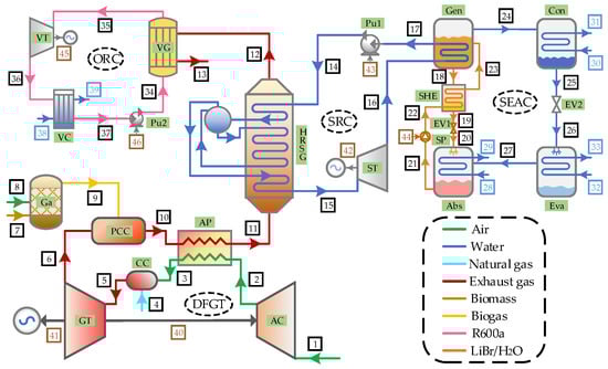
Figure 1.
Schematic diagram of the proposed cogeneration system.
In the DFGT cycle, ambient air (stream 1) undergoes compression in an air compressor (AC), leading to its entry into the air preheater (AP) where it is heated by the flue gas (stream 10). Subsequently, the heated air (stream 3) reacts with the injected natural gas (stream 4) within the combustion chamber (CC), resulting in the production of high-temperature combustion products (stream 5) that are then expanded in the gas turbine (GT) to generate power. Additionally, the syngas (stream 9) derived from the biomass gasifier (Ga) is conveyed into the post-combustion chamber (PCC), where it undergoes a reaction with the oxygen present in the exhaust gas (stream 6) from the GT. This process leads to an elevation in both the mass flow rate and temperature of the flue gas. Subsequent to the release of heat to the compressed air within the AP, the high-temperature exhaust gas (stream 11) serves as the heat source for the bottoming heat recovery cycles.
In the bottoming cycles, the exhaust gas firstly flows through a heat recovery steam generator (HRSG), where the pressurized water (stream 14) absorbs heat to be converted into superheated vapor (stream 15). Then, it is expanded in the steam turbine (ST) to generate electricity. After that, the low-pressure vapor (stream 16) at the exit of the ST is condensed into saturated liquid (stream 17) in the generator (Gen) to supply the heat required for the SEAC. In the SEAC, the lithium bromide-water (LiBr-H2O) is employed as working pairs. The weak solution (stream 23) absorbs heat in the generator where it is separated into a strong solution (stream 18) and water vapor (stream 24). The strong solution passes through the solution heat exchanger (SHE) to preheat the weak solution (stream 22), and then, the low-temperature strong solution (stream 19) flows into the absorber (Abs) through an expansion valve (EV1). Meanwhile, the refrigerant vapor is condensed in the condenser (Con). The saturated liquid (stream 25) is throttled by an expansion valve (EV2) and flows into the evaporator (Eva), where it is evaporated to produce the cooling capacity. After that, the refrigerant vapor (stream 27) is absorbed by the strong solution (stream 20) in the absorber. Finally, the weak solution (stream 21) is pumped back to the generator.
The residual thermal energy of the exhaust gas is utilized by an ORC. In consideration of environmental impact and safety concerns, it is advisable to use working fluids that exhibit low global warming potential (GWP) and minimal ozone depletion potential (ODP) and are non-corrosive and non-flammable. Moreover, there is a risk associated with organic working fluids undergoing decomposition at elevated temperatures during direct heat exchange with exhaust gases, which could lead to component damage and safety hazards. In the context of the ORC loop, a working fluid that enhances cycle efficiency is selected. Research has demonstrated that R600a (isobutane) serves as an effective working fluid for low- to medium-temperature waste heat recovery, offering high power generation capacity and efficiency [31]. The decomposition temperature of R600a is relatively elevated, at approximately 300–320 °C [32], thereby eliminating the risk of decomposition when employing exhaust gas (stream 12) as the heat source. In addition to its operational advantages, R600a is also environmentally favorable, characterized by an ODP of 0 and a GWP of roughly 20 [33], making it a sustainable choice in line with environmental and safety standards.
In the ORC, the liquid working fluid (stream 34) undergoes a heating process in the vapor generator (VG) to reach its saturated vapor state (stream 35). Subsequently, it is expanded in the vapor turbine (VT) to generate power. After that, the exhaust vapor (stream 36) is subjected to condensation, transforming it into saturated liquid (stream 37) through the transfer of heat to the cooling water in the vapor condenser (VC). Ultimately, this saturated liquid is pressurized using pump (Pu2) before being returned to the vapor generator (VG).
3. System Modeling
In this section, mathematical models for the system are formulated by leveraging the principles of thermodynamics and economics. To facilitate the modeling process, the following assumptions are considered [34,35,36]:
- The processes operate under steady-state conditions;
- Changes in kinetic and potential energies and exergies are not taken into account;
- Heat losses from the components into the environment are negligible;
- Pressure drops in pipelines are excluded from consideration;
- The composition of ambient air is 21% oxygen and 79% nitrogen by volume;
- Ideal gas behavior is assumed for all gas mixtures;
- In the SEAC, the refrigerant leaving the evaporator or condenser is taken to be saturated, and the solutions at the outlet of the generator and absorber are in an equilibrium state corresponding to their temperatures and pressures;
- In the ORC, the working fluids leaving the vapor generator and condenser are treated as saturated vapor and liquid, respectively;
- Constant isentropic efficiencies are applied to pumps, turbines, and the compressor.
3.1. Energy Analysis
3.1.1. Combustion Chamber
In the combustion chamber, the natural gas reacts with the air. The chemical equation for a complete combustion is presented as follows [18]:
The energy balance equation for an adiabatic combustion is expressed as follows:
where and are the enthalpy of formation and the difference in specific enthalpy for the jth component, respectively. The coefficients to refer to the kilomoles of the constituents.
3.1.2. Biomass Gasifier
To forecast the composition of the producer gas, the equilibrium model is utilized, predicated on the assumption that all chemical reactions attain thermodynamic equilibrium and that the pyrolysis products reach a state of balance in the reduction zone prior to their departure from the gasifier. The overarching reaction of gasification for biomass fuel is formulated as follows: [18,37]:
where CHaObNc stands for the chemical formula of the biomass, w is the moisture content of biomass, and is the kilomoles of oxygen in the air participating in the reaction.
The moisture level in the biomass is quantifiable based on the mass-based moisture content (MC), which is defined as follows: [18]:
where and are the molecular weights of the biomass and water, respectively. In this study, the type of biomass is wood (CH1.44O0.66, MC = 20%) [15,18,37].
In the gasification process, the main chemical reactions are shown as follows [18]:
Equations (5) and (6) can be combined to give the water-gas shift reaction [18]:
The equilibrium constants for Equations (7) and (8) are defined as follows [35]:
where PGa is the gasification pressure. K1 and K2 are related to the change in the Gibbs functions for the corresponding reactions, shown as follows [18]:
where is the universal gas constant, and is the gasifier temperature. and can be calculated based on the following [18]:
For an adiabatic process in the biomass gasifier, the energy balance equation at a given temperature can be expressed as follows [18]:
3.1.3. Post-Combustion Chamber
In the post-combustion chamber, the produced syngas reacts with the oxygen content of the exhaust gas at the outlet of the gas turbine. The following equation can be applied for a complete combustion reaction [18]:
where is the kilomoles of the biomass entering the gasifier.
Assuming an adiabatic combustion process, the energy balance for the reaction is given by the following:
where is the kilomoles of the jth component in the syngas, exhaust gas from the combustion chamber, or exhaust gas from post-combustion chamber.
3.1.4. Other System Components
The general form of the steady-state governing equations of the mass balance, energy balance, and concentration balance for each component of the system can be written as follows [35]:
where X denotes the mass concentration of LiBr in the solution.
The mass and energy balance equations for the components of the proposed system are presented in Table 1.

Table 1.
Mass and energy balance equations for the system components.
3.2. Exergy Analysis
The exergy balance equation for each component can be written as follows [38]:
where , , , and are the rates of supplied fuel, generated product, exergy destruction and exergy loss, respectively. The exergy balance equations for the system components are presented in Table 2.
Table 2.
Exergy balance equations for the system components.
The exergy content in a fluid stream is composed of four components: physical exergy, chemical exergy, kinetic exergy, and potential exergy. If the kinetic and potential aspects are disregarded, the stream’s specific exergy can be represented as follows [38]:
where and are the specific chemical exergy and specific physical exergy respectively, defined as follows [38]:
where and denote the mole fraction and standard chemical of ith component, respectively.
The specific chemical exergy of a solid biomass fuel is determined based on the following [18]:
where represents the proportion of chemical exergy to the lower heating value (LHV) of the biomass’s organic fraction, calculated as follows [18]:
where MO, MC, and MH are the mass fractions of oxygen, carbon, and hydrogen, respectively. The LHVs of dry biomass and natural gas are 18,732 kJ/kg and 50,020 kJ/kg, respectively [15].
The exergy efficiency of kth component is characterized based on the following [38]:
The exergy destruction ratio is characterized as the proportion of exergy destruction in the kth component relative to the system’s overall exergy destruction [38]:
3.3. Exergoeconomic Analysis
An exergoeconomic analysis combines an exergy analysis with economic principles to reveal the cost formation process and calculate the cost per exergy unit of the product. For each component, the cost balance equation can be expressed as follows [38]:
In which,
where represents the cost rate ($/h), and stands for the cost per unit of exergy ($/GJ). denotes the aggregate cost rate for the kth component, encompassing capital investment, operating, and maintenance expenses, and is computed as detailed below [39]:
where is the capital cost of the kth component, and and N are the maintenance factor (1.06) and annual operating hours (8000). CRF indicates the capital recovery factor, which is computed based on the following [39]:
where ir is the annual interest rate (5%), and nt is the lifetime of the system (20 years).
The average unit cost of the fuel (), unit cost of the product (), and cost rate of exergy destruction () for the kth component are respectively given as follows [38]:
The relative cost difference (rk) and exergoeconomic factor (fk) for the kth component are respectively defined as follows [38]:
The total cost rate (TCR) of the system is calculated as follows [23,39]:
In order to evaluate the component costs of the heat exchangers, the heat transfer areas (Ak) should be determined first, which is calculated based on the following [19]:
where represents the logarithmic mean temperature difference, and Uk denotes the heat transfer coefficient. The equations used to calculate the heat transfer coefficients of heat exchangers are listed in Appendix A.
The cost balance and auxiliary equations for the system components are presented in Table 3. The cost functions applied to estimate the capital costs of the system components are listed in Appendix B. All the cost values are calculated at their reference years (), and they should be updated to the values at the present year () using the chemical engineering plant cost index (CEPCI) based on the following relation [19]:
Table 3.
Cost balance and auxiliary equations for the system components.
3.4. Overall Performance Assessment
The thermal efficiency of the cogeneration system is defined as follows:
The exergy efficiency of the cogeneration system is computed based on the following:
The sum unit cost of the product (SUCP) of the cogeneration system is given by the following:
3.5. Multi-Objective Optimization
Optimization is widely recognized as a prevalent method in energy system design. Within the scope of an actual engineering project, it is essential to holistically consider all evaluation criteria, thereby capturing the system’s performance across various dimensions. The multi-objective optimization technique is particularly beneficial for addressing problems with two or more, potentially conflicting, objective functions simultaneously. The optimization procedure is initiated with the definition of objective functions, followed by the identification of decision variables and their respective boundaries, which can be formulated as follows [40]:
subject to
where X, F(X), and f(X) are the vectors of decision variables, the multi-objective function, and the single-objective function, respectively; and are the inequality and equality constraints, respectively; and and are the bottom and top bounds of the kth decision variables, respectively.
The multi-objective optimization problems can be solved using a genetic algorithm (GA). This method is inspired by evolutionary biology, which adopts a stochastic and global comprehensive search strategy to locate optimal solutions [41].
This procedure begins with the generation of a random initial population, which subsequently undergoes evolutionary operations, such as selection, mutation, crossover, and inheritance. Through successive generations, this population gravitates towards optimal solutions [42]. GA identifies a set of optimal solutions, constituting a Pareto frontier, where each solution is a balanced compromise among different objectives, with none being dominant as the simultaneous improvement of objectives is not feasible.
For the selection of the final optimal solution, the TOPSIS (Technique for Order Preference by Similarity to Ideal Situation) decision-making approach is employed [43]. This technique aims to identify alternatives that are closest to the positive ideal solution (optimal value for each objective function) and farthest from the negative ideal solution (worst value for each objective function). The decision matrix formation and the calculation methods for determining the distance from both ideal and non-ideal solutions are formulated as follows [44]:
Finally, the solution exhibiting the highest value of Cli is chosen as the preferred final solution.
4. Results and Discussion
In this section, four sub-sections are arranged to display the results of the thermodynamic and exergoeconomic evaluation of the proposed system, including model validation, base case results, a parametric study, and multi-objective optimization. For the simulation, MATLAB R2018b software is utilized, and the properties of the working fluids are sourced from the REFPROP 9.0 database.
4.1. Model Validation
To corroborate the accuracy of the models developed in this study, the results from key subsystems, like the GT cycle, biomass gasifier, ORC, and SEAC, are contrasted with findings from prior research. The data in Table 4, Table 5, Table 6 and Table 7 show considerable concordance between the outcomes of this study and those documented in existing literature. This consistency underscores the reliability of the developed model in accurately predicting the performance of the proposed system.
Table 4.
Comparison of the simulation results of the GT cycle in this work with those reported by Khaljani et al. [39].
Table 5.
Comparison of the component percentages of the syngas obtained from this work and those reported in the literature (wood-CH1.44O0.66, MC = 20%, TGa = 1073.15 K).
Table 6.
Comparison of the results obtained from this work with those reported by Saleh et al. [46] for the ORC cycle using R600a as the working fluid.
Table 7.
Comparison of the simulation results of the LiBr-H2O SEAC in this work with those reported by Nondy et al. [30] under the same operating conditions ( = 3.51 kW, Tgen = 363.15 K, Teva = 280.15 K, Tabs = 313.15 K, Tcon = 313.15 K, = 0.8).
4.2. Base Case Results
Table 8 details the input parameters for the four subsystems. Utilizing these values and resolving the associated mathematical equations yields the simulation outcomes. The thermodynamic and economic characteristics of each stream are catalogued in Table 9, while Table 10 displays the distribution of exergy and exergoeconomic parameters across the cogeneration system’s components. The findings highlight that the air compressor incurs the highest investment cost rate at 15.50 $/h, with the HRSG and gas turbine following at 11.15 $/h and 10.87 $/h, respectively. From an exergy perspective, the gas turbine and air compressor exhibit superior performance, both exceeding 90% in exergy efficiency, whereas the SEAC’s absorber demonstrates the lowest exergy efficiency at 14.41%.
Table 8.
Input parameters for the proposed system.
Table 9.
Thermodynamic properties and costs of the streams for the system.
Table 10.
Exergy and exergoeconomic factors for the system.
Figure 2 and Figure 3 illustrate the contributions to the exergy destruction rate and the cost associated with exergy destruction across the system components, respectively. As can be seen, the combustion chamber leads in the exergy destruction rate, contributing to 30.51% of the system’s total exergy destruction, followed closely by the post-combustion chamber. This high rate of exergy destruction, coupled with the significant fuel cost rate, also makes the combustion chamber the highest cost of exergy destruction.
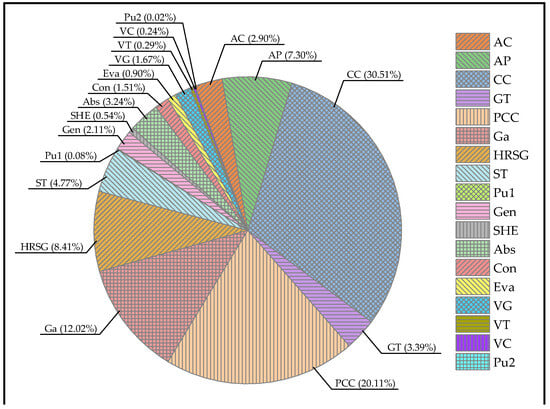
Figure 2.
Contribution of each component of the system to the exergy destruction rate.
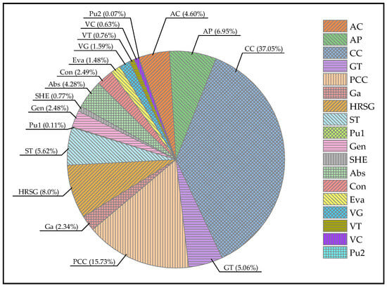
Figure 3.
Contribution of each component of the system to the cost of exergy destruction.
Table 11 presents the thermodynamic and exergoeconomic evaluation results of the cogeneration system in the base case. The results suggest that the system can produce a net power of 9206.7 kW and a cooling capacity of 6621 kW. Taking into account the operating hours per year, the annual power and cooling production are estimated to be 73,653.8 MW·h and 190,685.0 GJ, respectively. The overall energy efficiency, exergy efficiency, and SUCP stand at 75.69%, 41.76%, and 13.37 $/GJ, respectively. Moreover, the unit cost of power generated by the ORC turbine (32.39 $/GJ) significantly surpasses that of the gas turbine (14.06 $/GJ) and the SRC turbine (12.52 $/GJ), while the unit cost of the cooling product is comparatively lower, at 9.70 $/GJ.
Table 11.
Thermodynamic and exergoeconomic evaluation results of the base case.
4.3. Parametric Study
4.3.1. Effect of Air Compressor Pressure Ratio on the System Performance
Figure 4 presents the effect of the air compressor pressure ratio (PRAC) on the system performance. With the increase in the PRAC, the thermal and exergy efficiencies reach their peak values at a higher value of the PRAC of about 14 and decrease subsequently. On the contrary, the SUCP reaches its nadir when the value of PRAC is around 9 and then increases. The trends can be explained by the fact that the system performance depends on the performance of DFGT because the efficiencies of the bottoming cycles are kept unchanged due to fixed operating parameters. According to the DFGT, the thermal heat supplied by natural gas and biomass is minimal at a specific PRAC under the constant output power. At this point, the DFGT exhibits the highest thermal and exergy efficiencies, while the mass flow rate of exhaust gas is at its lowest. Consequently, the net power output and cooling capacity, as well as exergy destruction, have minimum values.
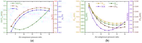
Figure 4.
Effect of air compressor pressure ratio on the (a) thermal efficiency, exergy efficiency, and SUCP; (b) net power output, cooling output, exergy destruction, and TCR of the proposed system.
4.3.2. Effect of Preheated Air Temperature on the System Performance
Figure 5 demonstrates the effect of the preheated air temperature (PAT) on the system performance. From Figure 5a, the negative correlations between PAT and thermal efficiency, exergy efficiency, and SUCP are observed. Meanwhile, as depicted in Figure 5b, the net power and cooling capacity, as well as exergy destruction of the system, present upward trends with an increase in the PAT. This is mainly due to the syngas consumption increasing as the PAT rises, leading to reduced system efficiency and an increased exhaust gas mass flow rate. Thus, the net power and cooling capacity increase because more thermal energy of exhaust gas could be utilized in the bottoming cycles.
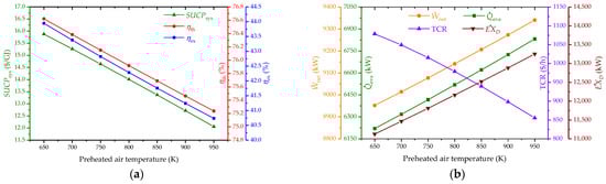
Figure 5.
Effect of preheated air temperature on the (a) thermal efficiency, exergy efficiency, and SUCP and (b) net power output, cooling output, exergy destruction, and TCR of the proposed system.
4.3.3. Effect of Gas Turbine Inlet Temperature on the System Performance
The impact of the gas turbine inlet temperature (GTIT) on the system performance is sketched in Figure 6. Observations from Figure 6a,b indicate that the thermal and exergy efficiencies are augmented with an increasing GTIT, while the net power and cooling capacity, as well as exergy destruction, decrease. This might be explained by the fact that, as the GTIT rises, the mass flow rate of the flue gas declines significantly due to the enthalpy difference through the gas turbine increasing when the power capacity of the DFGT is kept constant. As a consequence, the syngas consumption in the post-combustion chamber decreases dramatically as the GTIT is augmented, even though the natural gas consumption increases slightly, resulting in the reduction in total fuel consumption; thus, the energy and exergy efficiencies will increase. In addition, the net power and cooling capacity of the system decrease because less thermal heat is available for the bottoming cycles. The increase in the SUCP is mainly attributed to the increased investment cost of the gas turbine, which is very sensitive to the higher GTIT.
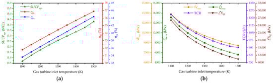
Figure 6.
Effect of the gas turbine inlet temperature on the (a) thermal efficiency, exergy efficiency, and SUCP and (b) net power output, cooling output, exergy destruction, and TCR of the proposed system.
4.3.4. Effect of Steam Turbine Inlet Pressure on the System Performance
The effect of the steam turbine inlet pressure (STIP) on the system performance is presented in Figure 7. As shown in Figure 7a, the exergy efficiency improves as the STIP rises, while the energy efficiency drops at first and then increases. According to Figure 7b, an elevation in the STIP results in an increase in net power owing to the improvement in the SRC efficiency. However, the reduction in SRC condensation heat leads to the decrease in cooling capacity. Consequently, the exergy efficiency improves, reflecting the higher quality of electricity production compared to cooling capacity.
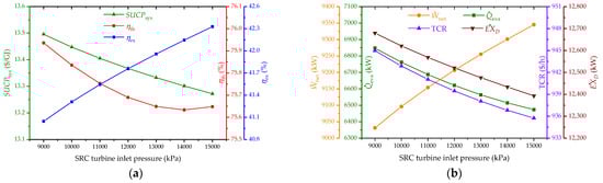
Figure 7.
Effect of steam turbine inlet pressure on the (a) thermal efficiency, exergy efficiency, and SUCP and (b) net power output, cooling output, exergy destruction, and TCR of the proposed system.
4.3.5. Effect of SRC Condensation Temperature on the System Performance
Figure 8 illustrates the influence of the SRC condensation temperature on the system performance. As shown in Figure 8a, an increase in the SRC condensation temperature results in an increase in the SUCP and a decrease in exergy efficiency, while the thermal efficiency will be maximized. According to Figure 8b, the net power declines as the SRC condenser temperature rises owing to the decrease in SRC efficiency, while the cooling capacity of the SEAC is augmented due to its COP and the input heat increase. System thermal efficiency is contingent on the combined output of the power and cooling capacity. Meanwhile, the output exergy declines as the net power drops because the quality of electricity is higher than that of the cooling capacity, which causes the exergy efficiency to decrease. Moreover, the SUCP and TCR increase slightly because the investment costs of SEAC components become higher.
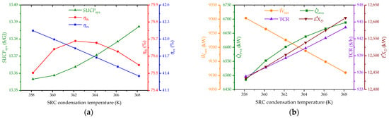
Figure 8.
Effect of SRC condensation temperature on the (a) thermal efficiency, exergy efficiency, and SUCP and (b) net power output, cooling output, exergy destruction, and TCR of the proposed system.
4.3.6. Effect of ORC Turbine Inlet Pressure on the System Performance
The effect of the ORC turbine inlet pressure on the system performance is presented in Figure 9. Obviously, changes in the ORC turbine inlet pressure do not affect the topping cycles, with variations only observed in the bottoming ORC cycle. According to Figure 9, slight increases in thermal and exergy efficiencies, as well as SUCP, are noted with the rise in the ORC turbine inlet pressure. In general, the ORC turbine inlet pressure has little influence on the system performance because the power produced by the ORC constitutes a small fraction of the total output power.
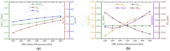
Figure 9.
Effect of the ORC turbine inlet pressure on the (a) thermal efficiency, exergy efficiency, and SUCP and (b) net power output, cooling output, exergy destruction, and TCR of the proposed system.
4.4. Optimization Results
This section outlines the findings from a multi-objective optimization process, aimed at identifying the best operating parameters for the system under consideration. The primary goals of this optimization are to enhance exergy efficiency and minimize the specific SUCP, addressing both thermodynamic and economic factors. Key operating parameters and their respective limits, ascertained through a parametric study, are detailed in Table 12. A Genetic Algorithm (GA) process, formulated in MATLAB, is employed for this dual-objective optimization task. Figure 10 presents the Pareto frontier derived from these optimization results, where each point signifies an optimal solution. Notably, an increase in exergy efficiency corresponds to an increase in the SUCP, revealing a distinct compromise between these two objectives. The peak exergy efficiency is achieved at point A, whereas the lowest SUCP is found at point B. To pinpoint the most suitable final optimal solution, the TOPSIS method is applied, resulting in the selection of point C as the ultimate choice. Table 13 displays the values for the objective functions and decision variables at points A, B, and C on the Pareto frontier.
Table 12.
Selected decision variables of the proposed system and their limits.

Figure 10.
Pareto frontier for two-objective optimization based on the exergy efficiency and SUCP.
Table 13.
The values of decision variables and objective functions at points A, B, and C.
5. Conclusions
In this study, the combination of the SRC, SEAC, and ORC as a cogeneration system is suggested for the waste heat recovery of a DFGT cycle fed by natural gas and biomass. A detailed thermodynamic and exergoeconomic evaluation, parametric analysis, and two-objective optimization of the system have been carried out. The main conclusions are summarized as follows:
- (1)
- In the baseline scenario, the system achieves the overall energy efficiency, exergy efficiency, and SUCP of the system of 75.69%, 41.76%, and 13.37 $/GJ respectively. Concurrently, it generates net power and cooling capacities of 9206.7 kW and 6621 kW.
- (2)
- Within the system, the combustion chamber is the primary contributor to the exergy destruction rate, followed closely by the post-combustion chamber. These two components also significantly contribute to the cost of exergy destruction.
- (3)
- Optimal thermal and exergy efficiencies are achieved at a higher air compressor pressure ratio of approximately 14, while the lowest SUCP is observed at a pressure ratio near 9.
- (4)
- Improvements in thermal and exergy efficiencies can be achieved by increasing the gas turbine inlet temperature or decreasing the preheated air temperature at the expense of economic performance deterioration.
- (5)
- The system performs better regarding exergy efficiency and SUCP at a higher SRC inlet pressure or lower SRC condensation temperature.
- (6)
- Under the optimal operating conditions, the system achieves an enhancement in exergy efficiency by 0.3% and a decrease in the SUCP by 2.8%, relative to the baseline scenario.
The primary challenge of DFGT-based cogeneration systems lies in their complexity, which poses significant issues for maintaining reliability and stability. Addressing this requires advanced control strategies and expert management, as complexity tends to increase maintenance demands and operational costs, thereby impacting the economic feasibility of the system. Future research could focus on developing dynamic simulation models to thoroughly analyze the system’s behavior under varying operational conditions. Such studies would be crucial in assessing the system’s stability and adaptability, thus providing deeper insight into its practical effectiveness and long-term sustainability. Additionally, incorporating real-time operational data in future research could significantly enhance the precision and validity of these dynamic models.
Author Contributions
Conceptualization, J.L. and J.R.; methodology, J.L.; software, J.L. and J.R.; validation, J.R. and L.L.; formal analysis, J.L., Y.Z. and C.X.; investigation, J.L., C.X. and L.L.; writing—original draft preparation, J.L., Y.Z. and W.H.; writing—review and editing, J.R.; project administration, J.L. and J.R.; funding acquisition, J.L. All authors have read and agreed to the published version of the manuscript.
Funding
This research was funded by the Natural Science Foundation of Hubei Province, grant number 2023AFB579. The APC was funded by Wuhan Business University.
Data Availability Statement
Data are contained within the article.
Conflicts of Interest
The authors declare no conflict of interest.
Nomenclature
| A | area (m2) | DFGT | dual fuel gas turbine |
| cost per exergy unit ($·GJ−1) | EV | expansion valve | |
| cost rate ($·h−1) | eva | evaporator | |
| ex | exergy per unit mass (kW·kg−1) | GA | genetic algorithm |
| exergy rate (kW) | Ga | gasifier | |
| f | exergoeconomic factor | gen | generator |
| h | specific enthalpy (kJ·kg−1) | GT | gas turbine |
| ir | annual interest rate (%) | GTIT | gas turbine inlet temperature |
| K | equilibrium constant | HRSG | heat recovery steam generator |
| mass flow rate (kg·s−1) | is | isentropic | |
| n | kilomoles of component (kmol) | LHV | lower heating value |
| N | annual operating hours (h) | MW | molecular weight |
| nt | lifetime of the system | ORC | organic Rankine cycle |
| P | pressure (kPa) | PAT | preheated air temperature |
| heat transfer rate (kW) | PCC | post combustion chamber | |
| r | relative cost difference | PR | pressure ratio |
| s | specific entropy (kJ·kg−1·K−1) | pu | pump |
| T | temperature (K) | SEAC | single-effect absorption chiller |
| U | heat transfer coefficient (W·m−2·K−1) | SHE | solution heat exchanger |
| power (kW) | SP | solution pump | |
| exergy destruction ratio (%) | SRC | steam Rankine cycle | |
| Z | investment cost ($) | ST | steam turbine |
| investment cost rate ($/h) | STIP | steam turbine inlet pressure | |
| SUCP | sum unit cost of the product | ||
| Subscript and abbreviations | VC | vapor condenser | |
| 0 | dead state | VG | vapor generator |
| 1,2,… | state points | VT | vapor turbine |
| abs | absorber | ||
| AC | air compressor | Greek Symbols | |
| AP | air preheater | η | efficiency |
| CC | combustion chamber | ε | heat exchanger effectiveness |
| con | condenser | maintenance factor | |
| COP | coefficient of performance | chevron angle | |
| CRF | capital recovery factor | chemical exergy coefficient | |
Appendix A
In this study, a fin-and-tube heat exchanger (FTHE) is chosen as the ORC vapor generator for its better performance under the condition that the heat transfer coefficients of the hot side (exhaust gas) and the cold side (working fluid) have a great difference [48]. The geometric dimensions of the FTHE are shown in and Table A1.
Table A1.
Geometric dimensions of the fin-and-tube heat exchanger.
Table A1.
Geometric dimensions of the fin-and-tube heat exchanger.
| Item | Value | Unit |
|---|---|---|
| Tube inner diameter, di | 20 | mm |
| Tube outer diameter, do | 25 | mm |
| Tube pitch, STu | 60 | mm |
| Fin height, HF | 12.5 | mm |
| Fin thickness,δF | 1 | mm |
| Fin pitch, YF | 4 | mm |
| Fouling factor [49,50] | ||
| Exhaust gas, rexh | m2·K−1·W | |
| Refrigerant (liquid), rliq | m2·K−1·W | |
| Refrigerant (vapor), rvap | m2·K−1·W | |
| Refrigerant (two-phase), rtp | m2·K−1·W | |
| Tube row alignment | Staggered type | |
| Tube and Fin material | Stainless steel 316 L | |
The vapor generator is mainly divided into a preheated zone and evaporation zone based on the working fluid state. The overall heat transfer coefficient for each zone can be calculated as follows [51]:
where αi and αo are heat transfer coefficient inside and outside tubes, respectively; λTu is the thermal conductivity of the tube material; γ is the rib effect coefficient; di and do are inner and outer diameters of the tube, respectively; ri and ro are fouling resistances inside and outside the tube, respectively; and ηo is the outside overall surface efficiency.
The plate heat exchanger (PHE) is suitable for the water-cooled condenser of the ORC, in which the heat transfer occurs between the low-pressure working fluid and the cooling water. The geometric dimensions of the PHE are illustrated in Table A2.
Table A2.
Geometric dimensions of the plate heat exchanger.
Table A2.
Geometric dimensions of the plate heat exchanger.
| Item | Value | Unit |
|---|---|---|
| Effective channel length, Le | 1250 | mm |
| Width of flow channel, Wch | 550 | mm |
| Plate thickness, δPl | 0.5 | mm |
| Mean flow channel gap, bch | 5 | mm |
| Corrugation pitch, Pco | 15 | mm |
| Chevron angle, β | π/3 | - |
| Plate material | Stainless steel 316 L | |
The condenser is divided into a precooled zone and condensation zone. The overall heat transfer coefficient for each zone of the plate heat exchanger is given as follows [52]:
where αhot and αcold are the convection heat transfer coefficients for the hot side and cold side, respectively; δPl is the thickness of plate; and λPl is the thermal conductivity of the plate material.
Based on the state of the working fluid, both the vapor generator and condenser can be divided into single-phase sections and two-phase sections. In the two-phase flow, the properties of the ORC working fluid vary with the vapor quality. In order to estimate the heat transfer coefficients, the two-phase sections of the evaporator and condenser are discretized and divided into some small parts so that constant thermodynamic properties can be assumed in each part. The correlations used for single-phase and two-phase heat transfer processes are presented in Table A3.
Table A3.
The correlations used to calculate the heat transfer coefficients of FTHE and PHE.
Table A3.
The correlations used to calculate the heat transfer coefficients of FTHE and PHE.
| Heat Exchanger Type | Heat Transfer Coefficient Correlation |
|---|---|
| Fin and tube heat exchanger | Young correlation for single-phase flow in shell side [53]: |
| Gnielinski correlation for single-phase flow in the tube side [54]: | |
| For liquid state: , | |
| For vapor state: , | |
| Liu-Winterton correlation for two-phase flow boiling in the tube [55]: | |
| Plate heat exchanger | Chisholm-Wanniarachchi correlation for single-phase flow [56]: |
| Han-Lee correlation for two-phase condensation [57]: | |
As for the SEAC, the constant heat transfer coefficients of the components are adopted according to the previous studies [58,59], listed in Table A4.
Table A4.
Heat transfer coefficients of the components in the SEAC.
Table A4.
Heat transfer coefficients of the components in the SEAC.
| Component | Heat Transfer Coefficient (W·m−2·K−1) |
|---|---|
| Generator | 1500 |
| Condenser | 2500 |
| Evaporator | 1500 |
| Absorber | 700 |
| SHE | 1000 |
Appendix B
In order to determine the capital costs of the system components in specific capacities and sizes, the following equations are used:
Air compressor [23,38]:
Air preheater [23,38]:
Combustion chamber [23,38]:
Gas turbine [23,38]:
Post combustion chamber [23,38]:
Biomass gasifier [23,35,36]:
Heat recovery steam generator [23,38]:
Generator [23,60]:
Condenser [23,60]:
Evaporator [23,60]:
Absorber [23,60]:
Solution heat exchanger Evaporator [23,60]:
Solution pump [23,60]:
The capital costs related to the pumps, turbines, FTHE, and PHE in the SRC or ORC are estimated using the following equations [61]:
where ZBM is the bare module cost (sum of direct and indirect costs for each component); FS is an additional factor for the overhead cost; FBM is a bare module factor; CP is the equipment purchase cost under base conditions; B1 and B2 are the constants for the different types of components; FM is the material factor; FP is the pressure factor; P is the operation pressure; and X is the capacity parameter, which refers to the heat transfer area of heat exchanger, the consumption power of the pump and the expansion power of the turbine, respectively. The coefficients of the above Equations (A16)–(A19) are listed in Table A5.
Table A5.
Coefficients of cost equations for the components.
Table A5.
Coefficients of cost equations for the components.
| Constant | Equipment | |||
|---|---|---|---|---|
| FTHE | PHE | Turbine | Pump | |
| 4.3247 | 4.6656 | 2.2659 | 3.3892 | |
| −0.3030 | −0.1557 | 1.4398 | 0.0536 | |
| 0.1634 | 0.1547 | −0.1776 | 0.1538 | |
| 0.0388 | 0 | 0 | −0.3935 | |
| −0.11272 | 0 | 0 | 0.3957 | |
| 0.08183 | 0 | 0 | −0.00226 | |
| 1.63 | 0.96 | 0 | 1.89 | |
| 1.66 | 1.21 | 1 | 1.35 | |
| 1.4 | 1 | 3.5 | 1.5 | |
| 1 | 1 | 1 | 1 | |
References
- Medeiros, D.L.; Sales, E.A.; Kiperstok, A. Energy production from microalgae biomass: Carbon footprint and energy balance. J. Clean. Prod. 2015, 96, 493–500. [Google Scholar] [CrossRef]
- Friedlingstein, P.; Andrew, R.M.; Rogelj, J.; Peters, G.P.; Canadell, J.G.; Knutti, R.; Luderer, G.; Raupach, M.R.; Schaeffer, M.; van Vuuren, D.P.; et al. Persistent growth of CO2 emissions and implications for reaching climate targets. Nat. Geosci. 2014, 7, 709–715. [Google Scholar] [CrossRef]
- Saidur, R.; Abdelaziz, E.A.; Demirbas, A.; Hossain, M.S.; Mekhilef, S. A review on biomass as a fuel for boilers. Renew. Sustain. Energy Rev. 2011, 15, 2262–2289. [Google Scholar] [CrossRef]
- International Energy Agency. Data and Statistics; International Energy Agency: Paris, France, 2020; Available online: https://www.iea.org/data-and-statistics/ (accessed on 27 July 2023).
- Soltani, S.; Mahmoudi, S.M.S.; Yari, M.; Rosen, M.A. Thermodynamic analyses of an externally fired gas turbine combined cycle integrated with a biomass gasification plant. Energy Convers. Manag. 2013, 70, 107–115. [Google Scholar] [CrossRef]
- Pantaleo, A.M.; Camporeale, S.M.; Shah, N. Thermo-economic assessment of externally fired micro-gas turbine fired by natural gas and biomass: Applications in Italy. Energy Convers. Manag. 2013, 75, 202–213. [Google Scholar] [CrossRef]
- Walter, A.; Llagostera, J. Feasibility analysis of co-fired combined-cycles using biomass-derived gas and natural gas. Energy Convers. Manag. 2007, 48, 2888–2896. [Google Scholar] [CrossRef]
- Amiri Rad, E.; Kazemiani-Najafabadi, P. Introducing a novel optimized Dual Fuel Gas Turbine (DFGT) based on a 4E objective function. J. Clean. Prod. 2019, 206, 944–954. [Google Scholar] [CrossRef]
- Franco, A.; Giannini, N. Perspectives for the use of biomass as fuel in combined cycle power plants. Int. J. Therm. Sci. 2005, 44, 163–177. [Google Scholar] [CrossRef]
- Fiaschi, D.; Carta, R. CO2 abatement by co-firing of natural gas and biomass-derived gas in a gas turbine. Energy 2007, 32, 549–567. [Google Scholar] [CrossRef]
- Riccio, G.; Chiaramonti, D. Design and simulation of a small polygeneration plant cofiring biomass and natural gas in a dual combustion micro gas turbine (BIO_MGT). Biomass Bioenergy 2009, 33, 1520–1531. [Google Scholar] [CrossRef]
- Gnanapragasam, N.V.; Reddy, B.V.; Rosen, M.A. Optimum conditions for a natural gas combined cycle power generation system based on available oxygen when using biomass as supplementary fuel. Energy 2009, 34, 816–826. [Google Scholar] [CrossRef]
- Pantaleo, A.M.; Camporeale, S.; Shah, N. Natural gas–biomass dual fuelled microturbines: Comparison of operating strategies in the Italian residential sector. Appl. Therm. Eng. 2014, 71, 686–696. [Google Scholar] [CrossRef]
- Barzegaravval, H.; Hosseini, S.E.; Wahid, M.A.; Saat, A. Effects of fuel composition on the economic performance of biogas-based power generation systems. Appl. Therm. Eng. 2018, 128, 1543–1554. [Google Scholar] [CrossRef]
- Soltani, S.; Mahmoudi, S.M.S.; Yari, M.; Morosuk, T.; Rosen, M.A.; Zare, V. A comparative exergoeconomic analysis of two biomass and co-firing combined power plants. Energy Convers. Manag. 2013, 76, 83–91. [Google Scholar] [CrossRef]
- Bhattacharya, A.; Manna, D.; Paul, B.; Datta, A. Biomass integrated gasification combined cycle power generation with supplementary biomass firing: Energy and exergy based performance analysis. Energy 2011, 36, 2599–2610. [Google Scholar] [CrossRef]
- Moharamian, A.; Soltani, S.; Rosen, M.A.; Mahmoudi, S.M.S. Advanced exergy and advanced exergoeconomic analyses of biomass and natural gas fired combined cycles with hydrogen production. Appl. Therm. Eng. 2018, 134, 1–11. [Google Scholar] [CrossRef]
- Soltani, S.; Mahmoudi, S.M.S.; Yari, M.; Rosen, M.A. Thermodynamic analyses of a biomass integrated fired combined cycle. Appl. Therm. Eng. 2013, 59, 60–68. [Google Scholar] [CrossRef]
- Gholizadeh, T.; Vajdi, M.; Rostamzadeh, H. A new biogas-fueled bi-evaporator electricity/cooling cogeneration system: Exergoeconomic optimization. Energy Convers. Manag. 2019, 196, 1193–1207. [Google Scholar] [CrossRef]
- Yilmaz, F.; Ozturk, M.; Selbas, R. Development and techno-economic assessment of a new biomass-assisted integrated plant for multigeneration. Energy Convers. Manag. 2019, 202, 112154. [Google Scholar] [CrossRef]
- Zhang, X.; Zeng, R.; Deng, Q.; Gu, X.; Liu, H.; He, Y.; Mu, K.; Liu, X.; Tian, H.; Li, H. Energy, exergy and economic analysis of biomass and geothermal energy based CCHP system integrated with compressed air energy storage (CAES). Energy Convers. Manag. 2019, 199, 111953. [Google Scholar] [CrossRef]
- Asgari, N.; Khoshbakhti Saray, R.; Mirmasoumi, S. Energy and exergy analyses of a novel seasonal CCHP system driven by a gas turbine integrated with a biomass gasification unit and a LiBr-water absorption chiller. Energy Convers. Manag. 2020, 220, 113096. [Google Scholar] [CrossRef]
- Zoghi, M.; Habibi, H.; Yousefi Choubari, A.; Ehyaei, M.A. Exergoeconomic and environmental analyses of a novel multi-generation system including five subsystems for efficient waste heat recovery of a regenerative gas turbine cycle with hybridization of solar power tower and biomass gasifier. Energy Convers. Manag. 2021, 228, 113702. [Google Scholar] [CrossRef]
- Liang, Y.; Shu, G.; Tian, H.; Wei, H.; Liang, X.; Liu, L.; Wang, X. Theoretical analysis of a novel electricity–cooling cogeneration system (ECCS) based on cascade use of waste heat of marine engine. Energy Convers. Manag. 2014, 85, 888–894. [Google Scholar] [CrossRef]
- Maryami, R.; Dehghan, A.A. An exergy based comparative study between LiBr/water absorption refrigeration systems from half effect to triple effect. Appl. Therm. Eng. 2017, 124, 103–123. [Google Scholar] [CrossRef]
- Liang, Y.; Shu, G.; Tian, H.; Sun, Z. Investigation of a cascade waste heat recovery system based on coupling of steam Rankine cycle and NH3-H2O absorption refrigeration cycle. Energy Convers. Manag. 2018, 166, 697–703. [Google Scholar] [CrossRef]
- Sahoo, U.; Kumar, R.; Singh, S.K.; Tripathi, A.K. Energy, exergy, economic analysis and optimization of polygeneration hybrid solar-biomass system. Appl. Therm. Eng. 2018, 145, 685–692. [Google Scholar] [CrossRef]
- Ahmadi, P.; Rosen, M.A.; Dincer, I. Greenhouse gas emission and exergo-environmental analyses of a trigeneration energy system. Int. J. Greenh. Gas Control 2011, 5, 1540–1549. [Google Scholar] [CrossRef]
- Anvari, S.; Khoshbakhti Saray, R.; Bahlouli, K. Conventional and advanced exergetic and exergoeconomic analyses applied to a tri-generation cycle for heat, cold and power production. Energy 2015, 91, 925–939. [Google Scholar] [CrossRef]
- Nondy, J.; Gogoi, T.K. Comparative performance analysis of four different combined power and cooling systems integrated with a topping gas turbine plant. Energy Convers. Manag. 2020, 223, 113242. [Google Scholar] [CrossRef]
- Paul Njock, J.; Ndame Ngangue, M.; Christian Biboum, A.; Thierry Sosso, O.; Nzengwa, R. Investigation of an organic Rankine cycle (ORC) incorporating a heat recovery water-loop: Water consumption assessment. Therm. Sci. Eng. Prog. 2022, 32, 101303. [Google Scholar] [CrossRef]
- Dai, X.; Shi, L.; An, Q.; Qian, W. Screening of hydrocarbons as supercritical ORCs working fluids by thermal stability. Energy Convers. Manag. 2016, 126, 632–637. [Google Scholar] [CrossRef]
- Wu, C.; Wang, S.-S.; Jiang, X.; Li, J. Thermodynamic analysis and performance optimization of transcritical power cycles using CO2-based binary zeotropic mixtures as working fluids for geothermal power plants. Appl. Therm. Eng. 2017, 115, 292–304. [Google Scholar] [CrossRef]
- Anvari, S.; Taghavifar, H.; Parvishi, A. Thermo- economical consideration of Regenerative organic Rankine cycle coupling with the absorption chiller systems incorporated in the trigeneration system. Energy Convers. Manag. 2017, 148, 317–329. [Google Scholar] [CrossRef]
- Balafkandeh, S.; Zare, V.; Gholamian, E. Multi-objective optimization of a tri-generation system based on biomass gasification/digestion combined with S-CO2 cycle and absorption chiller. Energy Convers. Manag. 2019, 200, 112057. [Google Scholar] [CrossRef]
- Cao, Y.; Mihardjo, L.W.W.; Dahari, M.; Tlili, I. Waste heat from a biomass fueled gas turbine for power generation via an ORC or compressor inlet cooling via an absorption refrigeration cycle: A thermoeconomic comparison. Appl. Therm. Eng. 2021, 182, 116117. [Google Scholar] [CrossRef]
- Zainal, Z.A.; Ali, R.; Lean, C.H.; Seetharamu, K.N. Prediction of performance of a downdraft gasifier using equilibrium modeling for different biomass materials. Energy Convers. Manag. 2001, 42, 1499–1515. [Google Scholar] [CrossRef]
- Bejan, A.; Tsatsaronis, G.; Moran, M. Thermal Design and Optimization; John Wiley & Sons: Hoboken, NJ, USA, 1996. [Google Scholar]
- Khaljani, M.; Khoshbakhti Saray, R.; Bahlouli, K. Comprehensive analysis of energy, exergy and exergo-economic of cogeneration of heat and power in a combined gas turbine and organic Rankine cycle. Energy Convers. Manag. 2015, 97, 154–165. [Google Scholar] [CrossRef]
- Feng, Y.; Zhang, Y.; Li, B.; Yang, J.; Shi, Y. Comparison between regenerative organic Rankine cycle (RORC) and basic organic Rankine cycle (BORC) based on thermoeconomic multi-objective optimization considering exergy efficiency and levelized energy cost (LEC). Energy Convers. Manag. 2015, 96, 58–71. [Google Scholar] [CrossRef]
- Ahmadi, P.; Dincer, I.; Rosen, M.A. Thermodynamic modeling and multi-objective evolutionary-based optimization of a new multigeneration energy system. Energy Convers. Manag. 2013, 76, 282–300. [Google Scholar] [CrossRef]
- Nazari, N.; Heidarnejad, P.; Porkhial, S. Multi-objective optimization of a combined steam-organic Rankine cycle based on exergy and exergo-economic analysis for waste heat recovery application. Energy Convers. Manag. 2016, 127, 366–379. [Google Scholar] [CrossRef]
- Hou, S.; Zhang, F.; Yu, L.; Cao, S.; Zhou, Y.; Wu, Y.; Hou, L. Optimization of a combined cooling, heating and power system using CO2 as main working fluid driven by gas turbine waste heat. Energy Convers. Manag. 2018, 178, 235–249. [Google Scholar] [CrossRef]
- Nazari, N.; Porkhial, S. Multi-objective optimization and exergo-economic assessment of a solar-biomass multi-generation system based on externally-fired gas turbine, steam and organic Rankine cycle, absorption chiller and multi-effect desalination. Appl. Therm. Eng. 2020, 179, 115521. [Google Scholar] [CrossRef]
- Roy, D.; Samanta, S.; Ghosh, S. Techno-economic and environmental analyses of a biomass based system employing solid oxide fuel cell, externally fired gas turbine and organic Rankine cycle. J. Clean. Prod. 2019, 225, 36–57. [Google Scholar] [CrossRef]
- Saleh, B.; Koglbauer, G.; Wendland, M.; Fischer, J. Working fluids for low-temperature organic Rankine cycles. Energy 2007, 32, 1210–1221. [Google Scholar] [CrossRef]
- Kaynakli, O.; Saka, K.; Kaynakli, F. Energy and exergy analysis of a double effect absorption refrigeration system based on different heat sources. Energy Convers. Manag. 2015, 106, 21–30. [Google Scholar] [CrossRef]
- Yang, F.; Zhang, H.; Bei, C.; Song, S.; Wang, E. Parametric optimization and performance analysis of ORC (organic Rankine cycle) for diesel engine waste heat recovery with a fin-and-tube evaporator. Energy 2015, 91, 128–141. [Google Scholar] [CrossRef]
- Kazemi, N.; Samadi, F. Thermodynamic, economic and thermo-economic optimization of a new proposed organic Rankine cycle for energy production from geothermal resources. Energy Convers. Manag. 2016, 121, 391–401. [Google Scholar] [CrossRef]
- Tian, H.; Chang, L.; Gao, Y.; Shu, G.; Zhao, M.; Yan, N. Thermo-economic analysis of zeotropic mixtures based on siloxanes for engine waste heat recovery using a dual-loop organic Rankine cycle (DORC). Energy Convers. Manag. 2017, 136, 11–26. [Google Scholar] [CrossRef]
- Yang, F.; Zhang, H.; Song, S.; Bei, C.; Wang, H.; Wang, E. Thermoeconomic multi-objective optimization of an organic Rankine cycle for exhaust waste heat recovery of a diesel engine. Energy 2015, 93, 2208–2228. [Google Scholar] [CrossRef]
- Imran, M.; Park, B.S.; Kim, H.J.; Lee, D.H.; Usman, M.; Heo, M. Thermo-economic optimization of Regenerative Organic Rankine Cycle for waste heat recovery applications. Energy Convers. Manag. 2014, 87, 107–118. [Google Scholar] [CrossRef]
- Zhang, H.G.; Wang, E.H.; Fan, B.Y. Heat transfer analysis of a finned-tube evaporator for engine exhaust heat recovery. Energy Convers. Manag. 2013, 65, 438–447. [Google Scholar] [CrossRef]
- Gnielinski, V. New equations for heat mass transfer in turbulent pipe and channel flows. Int. Chem. Eng. 1976, 16, 359–368. [Google Scholar]
- Liu, Z.; Winterton, R.H.S. A general correlation for saturated and subcooled flow boiling in tubes and annuli, based on a nucleate pool boiling equation. Int. J. Heat Mass Transf. 1991, 34, 2759–2766. [Google Scholar] [CrossRef]
- Ayub, Z.H. Plate heat exchanger literature survey and new heat transfer and pressure drop correlations for refrigerant evaporators. Heat Transf. Eng. 2003, 24, 3–16. [Google Scholar] [CrossRef]
- Han, D.H.; Lee, K.J.; Kim, Y.H. The characteristics of condensation in brazed plate heat exchangers with different chevron angles. J. Korean Phys. Soc. 2003, 43, 66–73. [Google Scholar]
- Mazzei, M.S.; Mussati, M.C.; Mussati, S.F. NLP model-based optimal design of LiBr–H2O absorption refrigeration systems. Int. J. Refrig. 2014, 38, 58–70. [Google Scholar] [CrossRef]
- Mussati, S.F.; Gernaey, K.V.; Morosuk, T.; Mussati, M.C. NLP modeling for the optimization of LiBr-H2O absorption refrigeration systems with exergy loss rate, heat transfer area, and cost as single objective functions. Energy Convers. Manag. 2016, 127, 526–544. [Google Scholar] [CrossRef]
- Misra, R.D.; Sahoo, P.K.; Sahoo, S.; Gupta, A. Thermoeconomic optimization of a single effect water/LiBr vapour absorption refrigeration system. Int. J. Refrig. 2003, 26, 158–169. [Google Scholar] [CrossRef]
- Turton, R.; Bailie, R.C.; Whiting, W.B.; Shaeiwitz, J.A.; Bhattacharyya, D. Analysis, Synthesis and Design of Chemical Processes, 4th ed.; Pearson Education: Upper Saddle River, NJ, USA, 2012. [Google Scholar]
Disclaimer/Publisher’s Note: The statements, opinions and data contained in all publications are solely those of the individual author(s) and contributor(s) and not of MDPI and/or the editor(s). MDPI and/or the editor(s) disclaim responsibility for any injury to people or property resulting from any ideas, methods, instructions or products referred to in the content. |
© 2023 by the authors. Licensee MDPI, Basel, Switzerland. This article is an open access article distributed under the terms and conditions of the Creative Commons Attribution (CC BY) license (https://creativecommons.org/licenses/by/4.0/).