


Reinforcement Learning-Based Multi-Objective of Two-Stage Blocking Hybrid Flow Shop Scheduling Problem

Abstract
:1. Introduction
- (1)
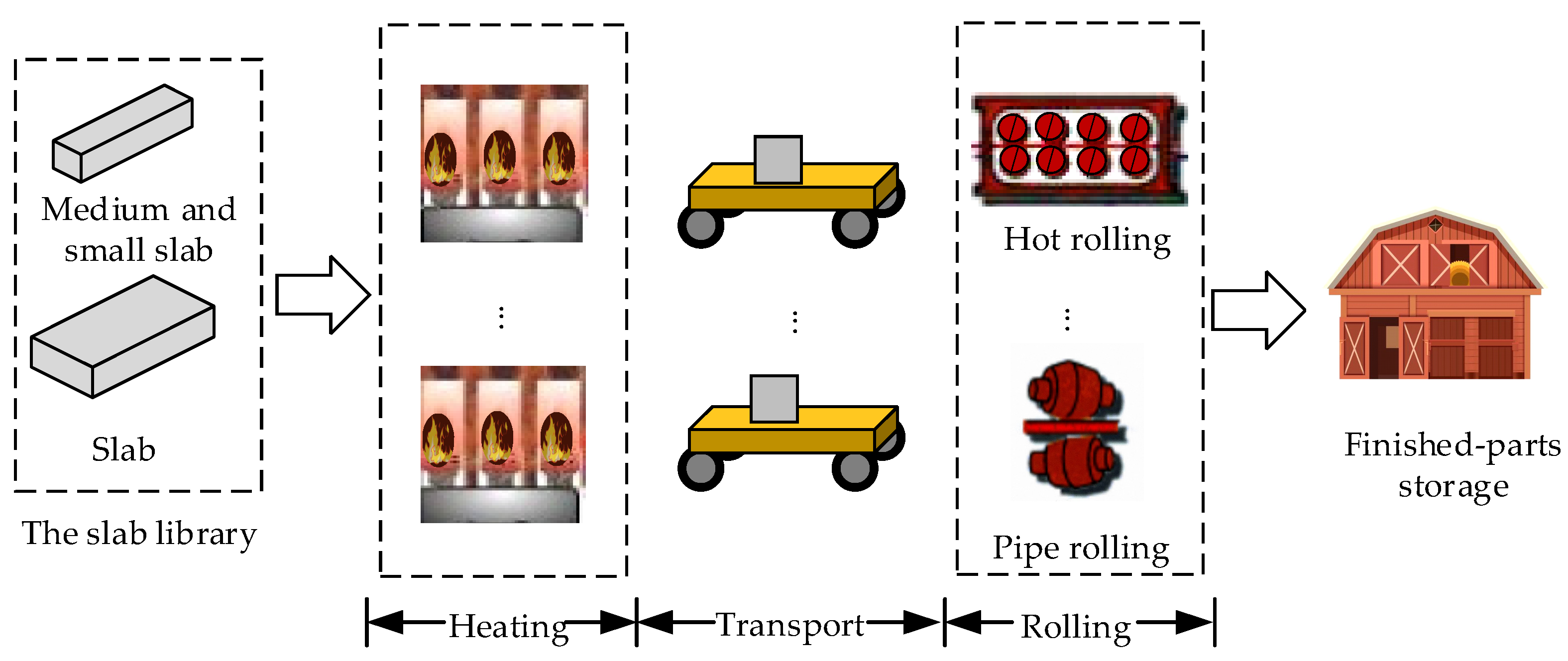
- For the problem of modern industrial process manufacturing, due to production process requirements, downstream machine congestion can result in upstream blocking, and the transportation time between upstream and downstream cannot be ignored. This paper formulates the HFSP with both transportation and blocking constraints. With the optimization objectives of minimizing the makespan and the total energy consumption, a two-stage BHFSP model incorporating transportation is established.
- (2)
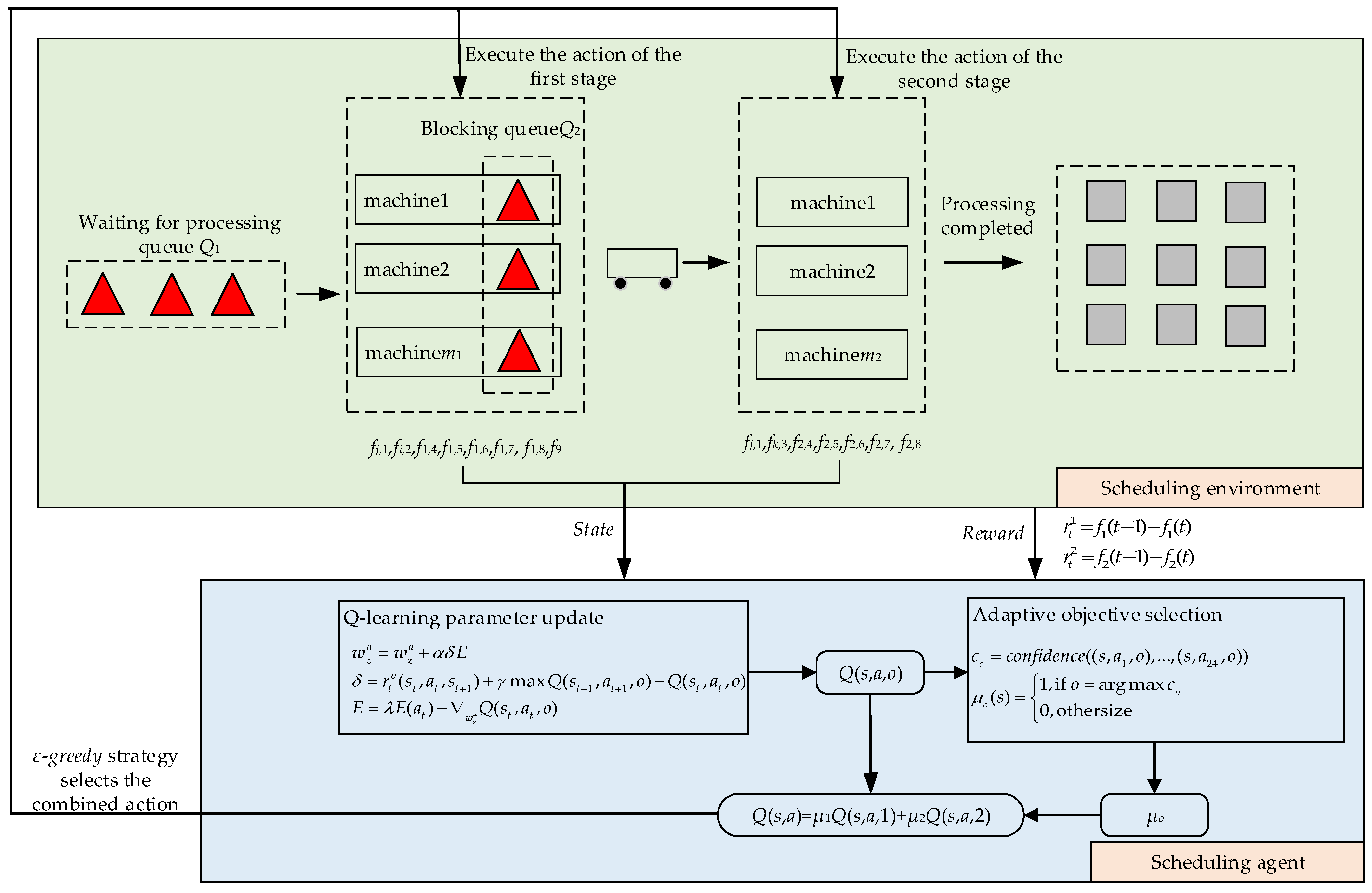
- We have designed an improved multi-objective Q-learning algorithm to address this model. Additionally, an adaptive object selection strategy based on t-tests has been developed for handling multi-objective optimization problems. This strategy coordinates the selection of different objectives by evaluating the confidence of the objective functions under the current job and machine state, thus optimizing both completion time and energy consumption indicators effectively.
2. Problem Formulation
- (1)
- All jobs have arrived at time zero and can begin processing.
- (2)
- There is no limit to the number of transport vehicles that can be used after the job leaves the first-stage machine.
- (3)
- Once the job begins processing or transporting, it cannot be interrupted.
- Makespan: The factors affecting the completion time of the job include processing time, transportation time, waiting processing time, and blocking time. The formula is defined as follows:
- 2.
- Total energy consumption: TEC includes blocking energy consumption (EC1), transportation energy consumption (EC2), and processing energy consumption (EC3). Notably, EC3 for each job is solely dependent on its processing time. Since each stage is equipped with identical parallel machines, EC3 is not affected by different processing sequences and remains constant. Therefore, Equation (6) shows that minimizing TEC requires minimizing EC1 and EC2. The second objective function is as follows:
3. Adaptive Objective Selection Q-Learning Algorithm
3.1. Problem Transformation
3.1.1. State
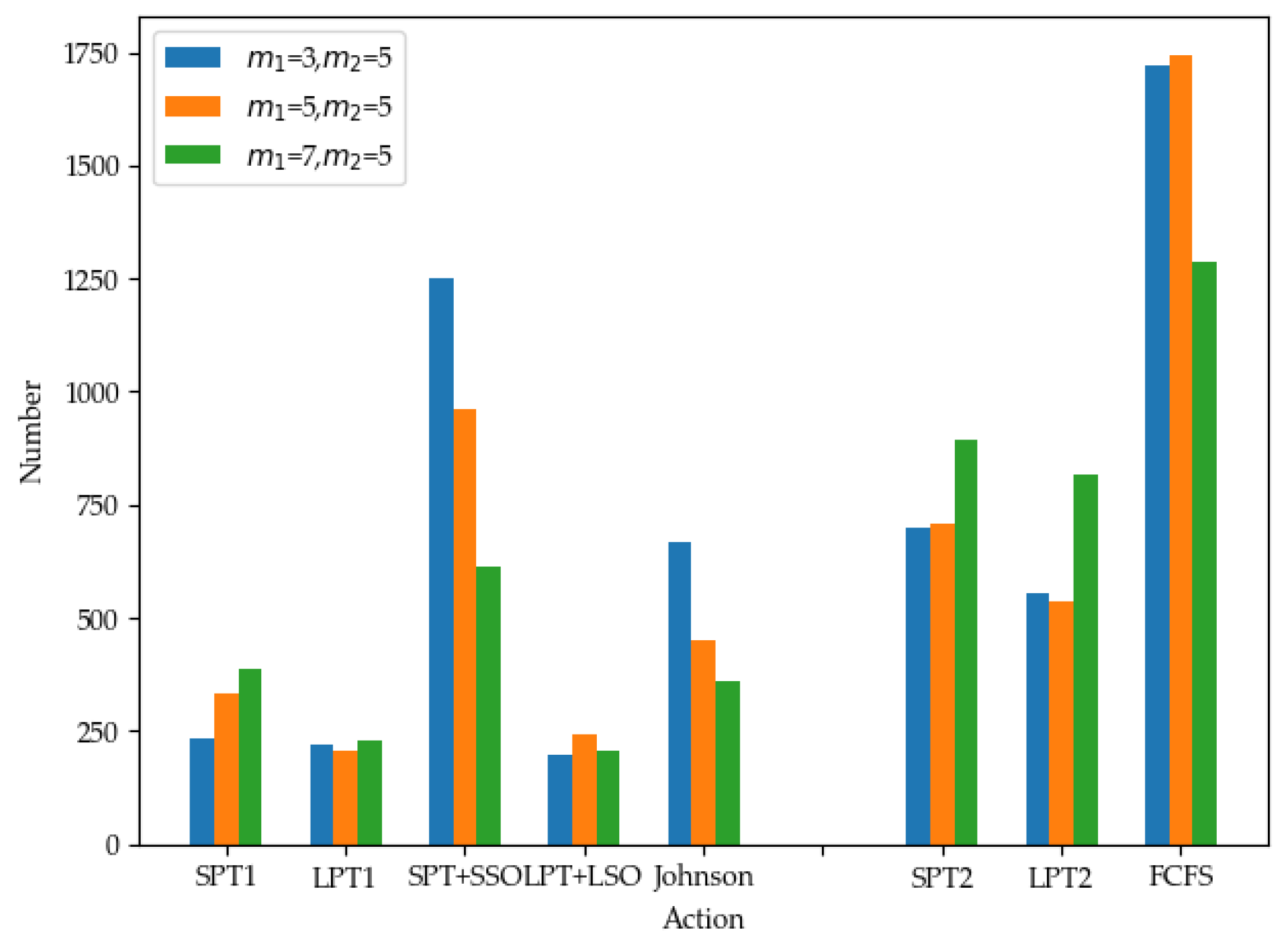
3.1.2. Action
- The First Production Stage
- The Second Production Stage
3.1.3. Reward
3.2. Value Function Approximation
3.3. T-Test-Based Adaptive Objective Selection
3.4. Algorithm Framework
4. Numerical Experiments
4.1. Experimental Environment and Parameter Setting
4.2. Experimental Results and Analysis
4.3. Experimental Comparison
5. Conclusions
Author Contributions
Funding
Data Availability Statement
Conflicts of Interest
References
- Cheng, Q.; Liu, C.; Chu, H.; Liu, Z.; Zhang, W.; Pan, J. A New Multi-Objective Hybrid Flow Shop Scheduling Method to Fully Utilize the Residual Forging Heat. IEEE Access 2020, 8, 151180–151194. [Google Scholar] [CrossRef]
- Wardono, B.; Fathi, Y. A tabu search algorithm for the multi-stage parallel machine problem with limited buffer capacities. Eur. J. Oper. Res. 2004, 155, 380–401. [Google Scholar] [CrossRef]
- Du, S.; Zhou, W.; Wu, D.; Fei, M. An effective discrete monarch butterfly optimization algorithm for distributed blocking flow shop scheduling with an assembly machine. Expert Syst. Appl. 2023, 225, 120113. [Google Scholar] [CrossRef]
- Miyata, H.H.; Nagano, M.S.; Gupta, J.N.D. Solutions methods for m-machine blocking flow shop with setup times and preventive maintenance costs to minimise hierarchical objective-function. Int. J. Prod. Res. 2023, 61, 6308–6335. [Google Scholar] [CrossRef]
- Cheng, C.-Y.; Pourhejazy, P.; Ying, K.-C.; Huang, S.-Y. New benchmark algorithm for minimizing total completion time in blocking flowshops with sequence-dependent setup times. Appl. Soft Comput. 2021, 104, 107229. [Google Scholar] [CrossRef]
- Zhao, F.; Shao, D.; Wang, L.; Xu, T.; Zhu, N.; Jonrinaldi. An effective water wave optimization algorithm with problem-specific knowledge for the distributed assembly blocking flow-shop scheduling problem. Knowl.-Based Syst. 2022, 243, 108471. [Google Scholar] [CrossRef]
- Niu, W.; Li, J. A two-stage cooperative evolutionary algorithm for energy-efficient distributed group blocking flow shop with setup carryover in precast systems. Knowl.-Based Syst. 2022, 257, 109890. [Google Scholar] [CrossRef]
- Zhao, F.; Xu, Z.; Bao, H.; Xu, T.; Zhu, N.; Jonrinaldi. A cooperative whale optimization algorithm for energy-efficient scheduling of the distributed blocking flow-shop with sequence-dependent setup time. Comput. Ind. Eng. 2023, 178, 109082. [Google Scholar] [CrossRef]
- Bao, H.; Pan, Q.; Ruiz, R.; Gao, L. A collaborative iterated greedy algorithm with reinforcement learning for energy-aware distributed blocking flow-shop scheduling. Swarm Evol. Comput. 2023, 83, 101399. [Google Scholar] [CrossRef]
- Nagano, M.; Takano, M.; Robazzi, J. A branch and bound method in a permutation flow shop with blocking and setup times. Int. J. Ind. Eng. Comput. 2022, 13, 255–266. [Google Scholar] [CrossRef]
- Wang, Y.; Wang, Y.; Han, Y. A Variant Iterated Greedy Algorithm Integrating Multiple Decoding Rules for Hybrid Blocking Flow Shop Scheduling Problem. Mathematics 2023, 11, 2453. [Google Scholar] [CrossRef]
- Qin, H.-X.; Han, Y.-Y.; Zhang, B.; Meng, L.-L.; Liu, Y.-P.; Pan, Q.-K.; Gong, D.-W. An improved iterated greedy algorithm for the energy-efficient blocking hybrid flow shop scheduling problem. Swarm Evol. Comput. 2022, 69, 100992. [Google Scholar] [CrossRef]
- Shao, Z.; Shao, W.; Pi, D. LS-HH: A learning-based selection hyper-heuristic for distributed heterogeneous hybrid blocking flow-shop scheduling. IEEE Trans. Emerg. Top. Comput. Intell. 2023, 7, 111–127. [Google Scholar] [CrossRef]
- Missaoui, A.; Boujelbene, Y. An effective iterated greedy algorithm for blocking hybrid flow shop problem with due date window. RAIRO-Oper. Res. 2021, 55, 1603–1616. [Google Scholar] [CrossRef]
- Aqil, S.; Allali, K. Two efficient nature inspired meta-heuristics solving blocking hybrid flow shop manufacturing problem. Eng. Appl. Artif. Intell. 2021, 100, 104196. [Google Scholar] [CrossRef]
- Qin, H.-X.; Han, Y.-Y.; Chen, Q.-D.; Li, J.-Q.; Sang, H.-Y. A double level mutation iterated greedy algorithm for blocking hybrid flow shop scheduling. Control Decis. 2022, 37, 2323–2332. [Google Scholar]
- Zhao, F.-Q.; Du, S.-L.; Cao, J.; Tang, J.-X. Study on distributed assembly blocking flow shop scheduling algorithm. J. Huazhong Univ. Sci. Technol. (Nat. Sci. Ed.) 2022, 50, 138–142+148. [Google Scholar]
- Wang, Y.; Jia, Z.; Zhang, X. A hybrid meta-heuristic for the flexible flow shop scheduling with blocking. Swarm Evol. Comput. 2022, 75, 101195. [Google Scholar] [CrossRef]
- Feng, Y.; Kong, J. Multi-Objective Hybrid Flow-Shop Scheduling in Parallel Sequential Mode While Considering Handling Time and Setup Time. Appl. Sci. 2023, 13, 3563. [Google Scholar] [CrossRef]
- Lei, D.; Su, B. A multi-class teaching–learning-based optimization for multi-objective distributed hybrid flow shop scheduling. Knowl.-Based Syst. 2023, 263, 110252. [Google Scholar] [CrossRef]
- Geng, K.; Wu, S.; Liu, L. Multi-objective re-entrant hybrid flow shop scheduling problem considering fuzzy processing time and delivery time. J. Intell. Fuzzy Syst. 2022, 43, 7877–7890. [Google Scholar] [CrossRef]
- Wu, X.; Cao, Z. An improved multi-objective evolutionary algorithm based on decomposition for solving re-entrant hybrid flow shop scheduling problem with batch processing machines. Comput. Ind. Eng. 2022, 169, 108236. [Google Scholar] [CrossRef]
- Wang, J.; Wang, L.; Cai, J.; Li, J.; Su, X. Solution Algorithm of Multi-objective Hybrid Flow Shop Scheduling Problem. J. Nanjing Univ. Aeronaut. Astronaut. 2023, 55, 544–552. [Google Scholar]
- Song, C. Improved NSGA-II algorithm for hybrid flow shop scheduling problem with multi-objective. Comput. Integr. Manuf. Syst. 2022, 28, 1777–17889. [Google Scholar]
- Lei, D.-M.; Wang, T. An improved shuffled frog leaping algorithm for the distributed two-stage hybrid flow shop scheduling. Control Decis. 2021, 36, 241–248. [Google Scholar]
- Song, C. A hybrid multi-objective teaching-learning based optimization for scheduling problem of hybrid flow shop with unrelated parallel machine. IEEE Access 2021, 9, 56822–56835. [Google Scholar] [CrossRef]
- Li, P.; Xue, Q.; Zhang, Z.; Chen, Z.; Zhou, D. Multi-objective energy-efficient hybrid flow shop scheduling using Q-learning and GVNS driven NSGA-II. Comput. Oper. Res. 2023, 159, 106360. [Google Scholar] [CrossRef]
- Wang, Y.; Wang, S.; Li, D.; Shen, C.; Yang, B. An improved multi-objective whale optimization algorithm for the hybrid flow shop scheduling problem considering device dynamic reconfiguration processes. Expert Syst. Appl. 2021, 174, 114793. [Google Scholar]
- Cui, H.; Li, X.; Gao, L.; Zhang, C. Multi-population genetic algorithm with greedy job insertion inter-factory neighbourhoods for multi-objective distributed hybrid flow-shop scheduling with unrelated-parallel machines considering tardiness. Int. J. Prod. Res. 2023, 1–19. [Google Scholar] [CrossRef]
- Wang, J.; Li, X.; Zhu, X. Intelligent dynamic control of stochastic economic lot scheduling by agent-based reinforcement learning. Int. J. Prod. Res. 2012, 50, 4381–4395. [Google Scholar] [CrossRef]
- Zhang, Z.; Zheng, L.; Li, N.; Wang, W.; Zhong, S.; Hu, K. Minimizing mean weighted tardiness in unrelated parallel machine scheduling with reinforcement learning. Comput. Oper. Res. 2012, 39, 1315–1324. [Google Scholar] [CrossRef]
- Lee, J.-H.; Kim, H.-J. Reinforcement learning for robotic flow shop scheduling with processing time variations. Int. J. Prod. Res. 2022, 60, 2346–2368. [Google Scholar] [CrossRef]
- Zhao, F.; Zhang, L.; Cao, J.; Tang, J. A cooperative water wave optimization algorithm with reinforcement learning for the distributed assembly no-idle flowshop scheduling problem. Comput. Ind. Eng. 2021, 153, 107082. [Google Scholar] [CrossRef]
- Zhang, C.; Song, W.; Cao, Z.; Zhang, J.; Tan, P.S.; Chi, X. Learning to dispatch for job shop scheduling via deep reinforcement learning. Adv. Neural Inf. Process. Syst. 2020, 33, 1621–1632. [Google Scholar]
- Li, Z.; Wei, X.; Jiang, X.; Pang, Y. A kind of reinforcement learning to improve genetic algorithm for multiagent task scheduling. Math. Probl. Eng. 2021, 2021, 1796296. [Google Scholar] [CrossRef]
- Luo, S. Dynamic scheduling for flexible job shop with new job insertions by deep reinforcement learning. Appl. Soft Comput. 2020, 91, 106208. [Google Scholar] [CrossRef]
- Zhang, J.; Cai, J. A Dual-Population Genetic Algorithm with Q-Learning for Multi-Objective Distributed Hybrid Flow Shop Scheduling Problem. Symmetry 2023, 15, 836. [Google Scholar] [CrossRef]
- Cheng, L.; Tang, Q.; Zhang, L.; Zhang, Z. Multi-objective Q-learning-based hyper-heuristic with Bi-criteria selection for energy-aware mixed shop scheduling. Swarm Evol. Comput. 2022, 69, 100985. [Google Scholar] [CrossRef]
- Chang, J.; Yu, D.; Zhou, Z.; He, W.; Zhang, L. Hierarchical Reinforcement Learning for Multi-Objective Real-Time Flexible Scheduling in a Smart Shop Floor. Machines 2022, 10, 1195. [Google Scholar] [CrossRef]
- Li, R.; Gong, W.; Lu, C. A reinforcement learning based RMOEA/D for bi-objective fuzzy flexible job shop scheduling. Expert Syst. Appl. 2022, 203, 117380. [Google Scholar] [CrossRef]
- Yuan, J.-L.; Chen, M.-C.; Jiang, T.; Li, C. Multi-objective reinforcement learning job scheduling method using AHP fixed weight in heterogeneous cloud environment. Control Decis. 2022, 37, 379–386. [Google Scholar]
- Wu, X.; Yan, X. An Improved Q Learning Algorithm to Optimize Green Dynamic Scheduling Problem in a Reentrant Hybrid Flow Shop. J. Mech. Eng. 2022, 58, 246–259. [Google Scholar]
- Wang, M.Y.; Sethi, S.P.; van de Velde, S.L. Minimizing makespan in a class of reentrant shops. Oper. Res. 1997, 45, 702–712. [Google Scholar] [CrossRef]


| α | γ | ε | λ | |
|---|---|---|---|---|
| K1 | 0.001 | 0.1 | 0.01 | 0.1 |
| K2 | 0.1 | 0.9 | 0.1 | 0.5 |
| K3 | 0.9 | 0.99 | 0.2 | 0.9 |
| No. | α | γ | ε | λ | Cmax | TEC | NP |
|---|---|---|---|---|---|---|---|
| 1 | 0.001 | 0.1 | 0.01 | 0.1 | 276 | 1548 | 1.84 |
| 2 | 0.001 | 0.9 | 0.1 | 0.5 | 268 | 1396 | 0.56 |
| 3 | 0.001 | 0.99 | 0.2 | 0.9 | 268 | 1396 | 0.56 |
| 4 | 0.1 | 0.1 | 0.1 | 0.9 | 266 | 1502 | 0.87 |
| 5 | 0.1 | 0.9 | 0.2 | 0.1 | 264 | 1380 | 0.18 |
| 6 | 0.1 | 0.99 | 0.01 | 0.5 | 271 | 1566 | 1.54 |
| 7 | 0.9 | 0.1 | 0.2 | 0.5 | 263 | 1538 | 0.80 |
| 8 | 0.9 | 0.9 | 0.01 | 0.9 | 276 | 1584 | 2.00 |
| 9 | 0.9 | 0.99 | 0.1 | 0.1 | 269 | 1356 | 0.46 |
| α | γ | ε | λ | |
|---|---|---|---|---|
| K1 | 2.96 | 3.51 | 5.38 | 2.49 |
| K2 | 2.59 | 2.74 | 1.89 | 2.89 |
| K3 | 3.26 | 2.56 | 1.54 | 3.43 |
| optimal | 0.1 | 0.99 | 0.2 | 0.1 |
| Job | Gurobi | AQL | ||||
|---|---|---|---|---|---|---|
| Cmax | TEC | T/s | Cmax | TEC | T/s | |
| n = 4 | 97 | 354 | 0.78 | 118 | 354 | 0.57 |
| n = 5 | 110 | 540 | 5.22 | 122 | 440 | 1.74 |
| n = 6 | 122 | 560 | 60 | 129 | 474 | 1.78 |
| n = 7 | 145 | 644 | 1195 | 149 | 542 | 2.60 |
| n = 8 | — | — | 1800 | 170 | 696 | 3.62 |
| Machine | Scheduling Solution | Cmax | TEC |
|---|---|---|---|
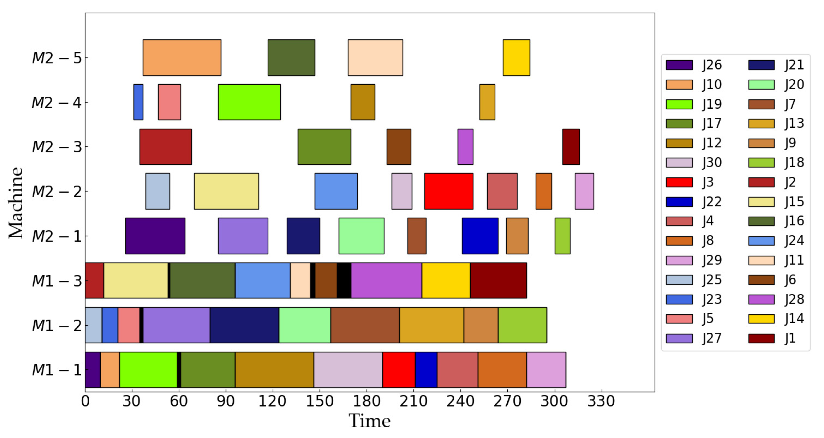
| m1 = 3, m2 = 5 | [26, 10, 19, 17, 12, 30, 3, 22, 4, 8, 29], [25, 23, 5, 27, 21, 20, 7, 13, 9, 18], [2, 15, 16, 24, 11, 6, 28, 14, 1] [26, 27, 21, 20, 7, 22, 9, 18], [25, 15, 24, 30, 3, 4, 8, 29], [2, 17, 6, 28, 1], [23, 5, 19, 12, 13], [10, 16, 11, 14] | 325 | 2218 |
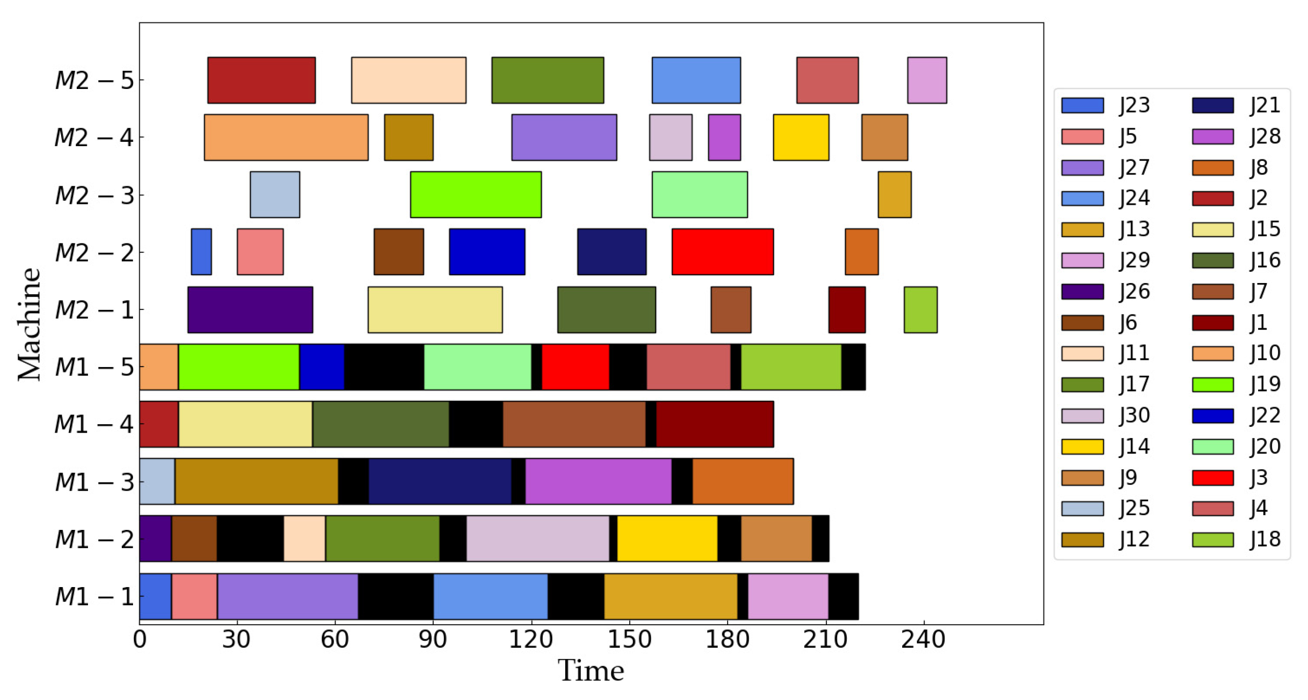
| m1 = 5, m2 = 5 | [23, 5, 27, 24, 13, 29], [26, 6, 11, 17, 30, 14, 9], [25, 12, 21, 28, 8], [2, 15, 16, 7, 1], [10, 19, 22, 20, 3, 4, 18] [26, 15, 16, 7, 1, 18], [23, 5, 6, 22, 21, 3, 8], [25, 19, 20, 13], [10, 12, 27, 30, 28, 14, 9], [2, 11, 17, 24, 4, 29] | 247 | 2838 |
| m1 = 7, m2 = 5 | [26, 23, 16, 7, 4], [25, 5, 29, 20, 8], [2, 3, 17, 28], [10, 19, 21, 13], [11, 9, 12, 18], [6, 27, 30, 1], [22, 15, 24, 14] [26, 23, 19, 12, 30], [25, 6, 3, 17, 7, 18, 1], [10, 27, 24, 14], [2, 22, 9, 15, 20, 28, 13], [11, 5, 29, 16, 21, 8, 4] | 237 | 3515 |
| No. | Rule | n = 15 | n = 30 | n = 50 | n = 100 | ||||
|---|---|---|---|---|---|---|---|---|---|
| Cmax | TEC | Cmax | TEC | Cmax | TEC | Cmax | TEC | ||
| R1 | SPT-SPT | 231 * | 1843 | 388 | 3461 | 615 | 5551 | 1236 | 11,585 |
| R2 | SPT-LPT | 231 * | 1843 | 374 | 3584 | 629 | 5379 | 1196 | 11,402 |
| R3 | SPT-FCFS | 231 * | 1843 | 388 | 3461 | 629 | 5379 | 1207 | 11,789 * |
| R4 | LPT-SPT | 213 | 1791 | 390 * | 3380 | 656 * | 6205 | 1185 | 10,028 |
| R5 | LPT-LPT | 214 | 1923 | 376 | 3289 | 650 | 5520 | 1235 | 11,638 |
| R6 | LPT-FCFS | 213 | 1791 | 384 | 3617 | 651 | 6212 | 1250 * | 11,557 |
| R7 | SPT + SSO-SPT | 214 | 1696 | 363 | 2398 | 586 | 5962 | 1181 | 11,277 |
| R8 | SPT + SSO-LPT | 214 | 1696 | 363 | 2398 | 577 | 5647 | 1178 | 10,478 |
| R9 | SPT + SSO-FCFS | 214 | 1696 | 363 | 2398 | 586 | 5962 | 1178 | 10,466 |
| R10 | LPT + LSO-SPT | 196 | 2097 * | 356 | 2979 | 553 | 5611 | 1165 | 11,329 |
| R11 | LPT + LSO-LPT | 196 | 2097 * | 344 | 3402 | 574 | 5780 | 1141 | 10,670 |
| R12 | LPT + LSO-FCFS | 196 | 2097 * | 356 | 2979 | 557 | 5701 | 1132 | 11,029 |
| R13 | Johnson-SPT | 194 | 1780 | 364 | 3653 * | 575 | 5730 | 1186 | 10,041 |
| R14 | Johnson-LPT | 194 | 1780 | 364 | 3653 * | 591 | 6418 | 1183 | 11,526 |
| R15 | Johnson-FCFS | 194 | 1780 | 364 | 3653 * | 577 | 6492 * | 1204 | 11,083 |
| R16 | AQL | 159 | 954 | 325 | 2218 | 511 | 4059 | 1098 | 8483 |
| No. | Rule | n = 15 | n = 30 | n = 50 | n = 100 | ||||
|---|---|---|---|---|---|---|---|---|---|
| Cmax | TEC | Cmax | TEC | Cmax | TEC | Cmax | TEC | ||
| R1 | SPT-SPT | 222 | 2248 | 317 | 4367 | 506 | 8006 | 1014 | 16,707 |
| R2 | SPT-LPT | 222 | 2248 | 286 | 4215 | 542 | 8552 | 1026 | 17,178 |
| R3 | SPT-FCFS | 222 | 2248 | 317 | 4367 | 541 | 8332 | 996 | 15,915 |
| R4 | LPT-SPT | 220 | 2837 | 323 | 4124 | 553 | 8987 | 1020 | 17,465 |
| R5 | LPT-LPT | 216 | 2884 | 327 * | 4767 * | 547 | 8913 | 1031 | 17,606 |
| R6 | LPT-FCFS | 224 * | 3364 * | 322 | 4648 | 567 * | 9078 | 1042 * | 17,655 |
| R7 | SPT + SSO-SPT | 180 | 1930 | 309 | 3952 | 514 | 7996 | 1025 | 16,060 |
| R8 | SPT + SSO-LPT | 180 | 1930 | 283 | 3291 | 525 | 8634 | 970 | 15,731 |
| R9 | SPT + SSO-FCFS | 180 | 1930 | 309 | 3952 | 526 | 8392 | 1018 | 15,741 |
| R10 | LPT + LSO-SPT | 186 | 2665 | 311 | 4208 | 513 | 8758 | 1018 | 17,777 |
| R11 | LPT + LSO-LPT | 186 | 2665 | 303 | 4276 | 523 | 8900 | 1000 | 16,819 |
| R12 | LPT + LSO-FCFS | 186 | 2665 | 287 | 3894 | 520 | 9389 * | 994 | 17,155 |
| R13 | Johnson-SPT | 168 | 2457 | 283 | 4043 | 470 | 8022 | 1026 | 18,701 * |
| R14 | Johnson-LPT | 168 | 2457 | 291 | 4496 | 491 | 9242 | 1026 | 18,555 |
| R15 | Johnson-FCFS | 168 | 2457 | 291 | 3957 | 491 | 9242 | 1000 | 17,756 |
| R16 | AQL | 151 | 1653 | 247 | 2838 | 440 | 7327 | 936 | 14,899 |
| No. | Rule | n = 15 | n = 30 | n = 50 | n = 100 | ||||
|---|---|---|---|---|---|---|---|---|---|
| Cmax | TEC | Cmax | TEC | Cmax | TEC | Cmax | TEC | ||
| R1 | SPT-SPT | 218 * | 3119 | 280 | 5624 | 496 | 10,688 | 1032 | 23,859 |
| R2 | SPT-LPT | 218 * | 3119 | 261 | 5464 | 486 | 10,571 | 1014 | 24,350 |
| R3 | SPT-FCFS | 218 * | 3119 | 280 | 5624 | 510 | 11,360 | 1005 | 22,438 |
| R4 | LPT-SPT | 212 | 3501 | 307 | 5256 | 559 * | 12,694 * | 1077 * | 25,128 |
| R5 | LPT-LPT | 212 | 3458 | 307 | 5914 | 551 | 11,466 | 1048 | 23,694 |
| R6 | LPT-FCFS | 212 | 3501 | 313 | 5737 | 551 | 11,466 | 1067 | 23,831 |
| R7 | SPT + SSO-SPT | 179 | 2382 | 258 | 3945 | 475 | 9553 | 1061 | 24,597 |
| R8 | SPT + SSO-LPT | 202 | 2689 | 296 | 5217 | 499 | 10,796 | 1048 | 25,348 |
| R9 | SPT + SSO-FCFS | 202 | 2689 | 260 | 4155 | 457 | 8329 | 1025 | 23,356 |
| R10 | LPT + LSO-SPT | 190 | 3729 | 312 | 6512 | 521 | 12,498 | 1049 | 26,380 * |
| R11 | LPT + LSO-LPT | 190 | 3729 | 327 * | 7087 | 510 | 11,741 | 1075 | 25,628 |
| R12 | LPT + LSO-FCFS | 190 | 3729 | 327 * | 7601 * | 510 | 11,741 | 1050 | 25,382 |
| R13 | Johnson-SPT | 190 | 3803 | 271 | 5192 | 481 | 10,031 | 1008 | 25,046 |
| R14 | Johnson-LPT | 201 | 3905 * | 286 | 5707 | 492 | 11,569 | 994 | 22,842 |
| R15 | Johnson-FCFS | 201 | 3905 * | 271 | 5192 | 482 | 11,593 | 991 | 22,391 |
| R16 | AQL | 177 | 1937 | 237 | 3515 | 455 | 9238 | 872 | 19,876 |
| No. | Job | Machine | NSGA-II | Q-Learning | AQL | |||
|---|---|---|---|---|---|---|---|---|
| Cmax | TEC | Cmax | TEC | Cmax | TEC | |||
| R1 | n = 15 | m1 = 3, m2 = 5 | 221 | 1330 | 161 | 1221 | 159 | 954 |
| R2 | n = 15 | m1 = 5, m2 = 5 | 165 | 2070 | 151 | 1661 | 151 | 1653 |
| R3 | n = 15 | m1 = 7, m2 = 5 | 149 | 2000 | 168 | 2115 | 177 | 1937 |
| R4 | n = 30 | m1 = 3, m2 = 5 | 410 | 2846 | 321 | 2359 | 325 | 2218 |
| R5 | n = 30 | m1 = 5, m2 = 5 | 254 | 3117 | 271 | 3215 | 247 | 2838 |
| R6 | n = 30 | m1 = 7, m2 = 5 | 239 | 3547 | 243 | 3895 | 237 | 3515 |
| R7 | n = 50 | m1 = 3, m2 = 5 | 704 | 4503 | 547 | 4527 | 511 | 4059 |
| R8 | n = 50 | m1 = 5, m2 = 5 | 445 | 7413 | 466 | 7403 | 440 | 7327 |
| R9 | n = 50 | m1 = 7, m2 = 5 | 456 | 10,187 | 475 | 9806 | 455 | 9238 |
| R10 | n = 100 | m1 = 3, m2 = 5 | 1356 | 9586 | 1132 | 9457 | 1098 | 8483 |
| R11 | n = 100 | m1 = 5, m2 = 5 | 983 | 15,037 | 973 | 14,945 | 936 | 14,899 |
| R12 | n = 100 | m1 = 7, m2 = 5 | 913 | 20,223 | 945 | 20,472 | 872 | 19,876 |
Disclaimer/Publisher’s Note: The statements, opinions and data contained in all publications are solely those of the individual author(s) and contributor(s) and not of MDPI and/or the editor(s). MDPI and/or the editor(s) disclaim responsibility for any injury to people or property resulting from any ideas, methods, instructions or products referred to in the content. |
© 2023 by the authors. Licensee MDPI, Basel, Switzerland. This article is an open access article distributed under the terms and conditions of the Creative Commons Attribution (CC BY) license (https://creativecommons.org/licenses/by/4.0/).
Share and Cite
Xu, K.; Ye, C.; Gong, H.; Sun, W. Reinforcement Learning-Based Multi-Objective of Two-Stage Blocking Hybrid Flow Shop Scheduling Problem. Processes 2024, 12, 51. https://doi.org/10.3390/pr12010051
Xu K, Ye C, Gong H, Sun W. Reinforcement Learning-Based Multi-Objective of Two-Stage Blocking Hybrid Flow Shop Scheduling Problem. Processes. 2024; 12(1):51. https://doi.org/10.3390/pr12010051
Chicago/Turabian StyleXu, Ke, Caixia Ye, Hua Gong, and Wenjuan Sun. 2024. "Reinforcement Learning-Based Multi-Objective of Two-Stage Blocking Hybrid Flow Shop Scheduling Problem" Processes 12, no. 1: 51. https://doi.org/10.3390/pr12010051
APA StyleXu, K., Ye, C., Gong, H., & Sun, W. (2024). Reinforcement Learning-Based Multi-Objective of Two-Stage Blocking Hybrid Flow Shop Scheduling Problem. Processes, 12(1), 51. https://doi.org/10.3390/pr12010051