Transfer Learning and Interpretable Analysis-Based Quality Assessment of Synthetic Optical Coherence Tomography Images by CGAN Model for Retinal Diseases

Abstract

This study investigates the effectiveness of using conditional generative adversarial networks (CGAN) to synthesize Optical Coherence Tomography (OCT) images for medical diagnosis. Specifically, the CGAN model is trained to generate images representing various eye conditions, including normal retina, vitreous warts (DRUSEN), choroidal neovascularization (CNV), and diabetic macular edema (DME), creating a dataset of 102,400 synthetic images per condition. The quality of these images is evaluated using two methods. First, 18 transfer-learning neural networks (including AlexNet, VGGNet16, GoogleNet) assess image quality through model-scoring metrics, resulting in an accuracy rate of 97.4% to 99.9% and an F1 Score of 95.3% to 100% across conditions. Second, interpretative analysis techniques (GRAD-CAM, occlusion sensitivity, LIME) compare the decision score distribution of real and synthetic images, further validating the CGAN network’s performance. The results indicate that CGAN-generated OCT images closely resemble real images and could significantly contribute to medical datasets.

1. Introduction

Optical coherence tomography (OCT) is based on the weak optical interferometer principle [1] and has been widely used in ophthalmology over the past ten years. OCT is capable of capturing various components of biological tissue, including the structural organization, molecular composition, elasticity modulus, and some other parameters of the organism, by the reflection and absorption of light [2]. These changes in biome parameters can be employed to identify various disorders, including oral epithelial dysplasia, as well as for blood oxygen measurement, blood glucose monitoring, plaque detection, and cancer [3,4]. OCT can be used to detect and diagnose eye problems on account of its high resolution and non-invasive nature. For instance, OCT is necessary for clinical decision making, monitoring macular and optic nerve illnesses, and precise determination of choroidal thickness. The World Vision Report (WVR) published by the World Health Organization (WHO) stated that more than 418 million people worldwide are afflicted with eye lesions that can lead to blindness [5], and this number will increase exponentially. The most prevalent disorders that cause vision loss in modern individuals are age-related macular degeneration (AMD) [6], choroidal neovascularization (CNV) [7], vitreous warts, and diabetic macular edema (DME) [8]. With the advancement of machine learning [9] and deep learning [10,11], increasingly high-precision models are employed to treat eye illnesses, merging this technology with current medicine to improve the decision-making capabilities of medical systems. These models include AlexNet [12], VGGNet [13], DarkNet [14], Inception [15], ResNet [16], DenseNet [17], MobileNet [18], NasNet [19], GoogleNet [20] and SqueezeNet [21]. However, these deep learning models always require large, clear, diversified, unique, and well-balanced images for model training, but the training data acquisition is a hurdle problem. Kermany et al. [22] used data from 108,312 photos of 4686 patients. The accuracy cannot be further improved due to the difficulty of obtaining huge quantities of medical data. According to the General Data Protection Regulation (GDPR) [23] of European member states, a variety of data, including eye pictures, are classified as biometric data and are considered private. The data are protected by law regardless of whether the participants give consent to the institution’s use of the data or not; it is difficult for the researcher to acquire large-scale OCT pictures for training purposes. To remedy the data deficiency, traditional data can be used to enrich the diversity of the training data (including rotating, panning, flipping, adding white noise, and adding masking [24]).

GAN [25], an advanced adversarial learning network, is also applied in the field of OCT image creation. Liu et al. [26] generated OCT images of AMD by combining GANs (DCGANs and WGANs architectures) with style transformation. Using the generated OCT images, Yanagihara et al. [27] trained a GAN to predict retinal abnormalities in untreated AMD patients. Burlina et al. [28] trained high-resolution OCT images of AMD using 133,821 color fundus photos to demonstrate that DCNNs can produce realistic fundus images. Zheng et al. [29] trained the OCT dataset on a publicly accessible GAN architecture and demonstrated that the genuine and synthetic OCT images owned comparable image quality. Using Fourier domain similarity, Tajmirriahi et al. [30] proposed a dual discriminator Fourier GAN (DDFAGAN) framework to generate more realistic OCT pictures. Seo et al. [31] developed a new GAN model for few-shot image generation, focusing on lifelong learning capabilities. You et al. [32] conducted a survey analyzing the use of GANs in ophthalmology, covering a range of tasks and identifying key challenges. Shaopeng Liu et al. [33] assessed six GAN models for predicting diabetic macular edema response to anti-VEGF therapy with OCT images, identifying RegGAN as the most precise in replicating post-treatment results. Furthermore, Xiaojun Yu et al. [34] developed MDR-GAN, a generative adversarial network incorporating multi-scale and dilated convolution res-network for OCT retinal image despeckling, demonstrating superior denoising performance compared to existing methods.

In this paper, four types of current fundus OCT data are trained using data augmentation [35] and conditional generative adversarial networks (CGAN) [36]. The fundus OCT dataset is augmented using conventional data augmentation techniques with CGAN; the expanded dataset is combined with the original dataset to form a new dataset (hybrid set), which is used as a training set for image fidelity verification in multiple transfer learning networks. Researchers have demonstrated that transfer learning [37] is an effective classification strategy that can achieve a more rapid training effect by fixing optimized low-level weight parameters. The output dataset quality of the CGAN network can be evaluated through different transfer learning models. CGAN, which is also an opaque model, can provide realistic data. Therefore, we attempted to employ GardCAM [38], LIME [39], and occlusion [40] techniques to analyze the interpretability of the CGAN-generated images [41]. The regions that CGAN concentrates on training when synthesizing images of particular retinal disorders are inferred in reverse by analyzing the regions that affect image evaluation in the synthesized images. Meanwhile, the quality of the synthesized image of the CGAN network can be further evaluated by comparing it with the interpretability of the real images.

The main contributions of this paper are summarized as follows:

(1)

A modified CGAN network is adopted to synthesize retinal OCT images for data augmentation.

(2)

Transfer learning is innovatively used as a quality evaluation mechanism for the generated image of CGAN.

(3)

Interpretable analysis approaches (GardCAM, LIME, and occlusion) are introduced for assessing the quality of retinal OCT pictures created by CGAN.

(4)

Theoretical results demonstrate that high-quality retinal OCT pictures generated by CGAN may function as a medical dataset.

The remainder of the paper is organized in further five sections: Section 2 examines the theoretical foundations of the modified CGAN network. Section 3 explains preprocessing methods and structural components of the CGAN network. The Section 4 summarizes the data sources and theoretical outcomes. Section 5 discusses strategies for evaluating the quality of CGAN synthetic images based on transfer learning and interpretability analysis methodologies. Section 6 displays the results and future research directions.

2. Theoretical Background

Conditional Generative Adversarial Networks

A GAN consists of two major components, such as a generator and a discriminator, D. The input generator, mapped by a random vector to a false image, is the likelihood of identifying whether the input image is fake. Assume that the used dataset is x. P_data(x) is the distribution of our dataset, p_z(z) is the distribution of random vectors, and P_g is the data distribution of the generator. The random vector output is indicated by G(z; θ_g), whereas the distribution of the dataset as x over the discriminator D is denoted by D(X; θ_d). The following is the loss function for the GAN [25].

$$\underset{G}{min}\underset{D}{max}V(D,G)=E_{x~p_{data\left(x\right)}}[\mathit{log}D(x)]+E_{z~p_{data\left(z\right)}}[\mathit{log}(1-D(G(z)))]$$

(1)

The original GAN can only generate images based on random vectors. Hence the discriminator can only be used to determine if the original GAN generated the input image. CGAN adds label input to the structure of the original GAN so that the connection between images and labels can be used during the training phase, and images with the relevant labels may be created during the testing phase. In the CGAN generator, the extra information y is added for restriction and is coupled to the random vector p_z(z) via a fully connected layer as the hidden layer input of the generator. As a discriminator for the hidden layer input, the input picture x is connected to the additional information y. The following is the CGAN loss function [36].

$$\underset{G}{min}\underset{D}{max}V(D,G)=E_{x~p_{data\left(x\right)}}[\mathit{log}D(x|y)]+E_{z~p_{data\left(z\right)}}[\mathit{log}(1-D(G(z|y)))]$$

(2)

It boils down to solving the difference between the distributions of P_data and P_g by sample. The objective is to identify an optimal generator G*, such that the difference between the distributions of P_data and P_g is minimized, and to derive the following equation for G*:

$$G^{*}=argmi{n}_{g}Div\left(P_g,P_{data}\right)$$

(3)

Instead of a generator, a novel discriminant D* is employed to solve the difference between the distributions of P_data and P_g, yielding the following equation:

$$D^{*}=argma{x}_{D}V(D,G)$$

(4)

At present, the optimization equation for G* is displayed below:

$$G^{*}=argmi{n}_{g}ma{x}_{D}V(G,D)$$

(5)

The main goal of the entire training procedure is to find the minimal JS divergence between the distributions Pdata and Pg. CGAN consists of a generator and a discriminator based on an optimized modification of GAN. Figure 1 illustrates the principle of CGAN. Figure 1 describes the structure of a Conditional Generative Adversarial Network (CGAN), which is an advanced type of Generative Adversarial Network (GAN) that includes additional label information for generating targeted synthetic data, like images, conditioned on these labels. This structure enhances the network’s ability to produce more specific and relevant outputs during the training process by adding additional label information to the generator and discriminator. The train phase creates images for the given labels and associates the labels with the images. Supervised learning is achieved by setting the labels as conditions.

3. Proposed Framework

In this section, the pre-processing of image data and the application of CGAN for generating synthetic images to enhance the original dataset are detailed as follows.

3.1. Data Pre-Processing

All OCT images will be preprocessed before being fed into the CGAN training network. The real dataset contains five image types with different pixel sizes. The shortest edge in each image type is used to determine the image length and width, and the image center is intercepted and interpolated to scale the image pixels to 256 × 256 to standardize the image size of the dataset. In addition, the image input to the CGAN must consist of three RGB channels. The images in the real dataset are grayscale maps with a single channel. All single-channel OCT greyscale images are converted to RGB images by copying the grayscale map channel pixels into the remaining two channels.

3.2. Modified CGAN

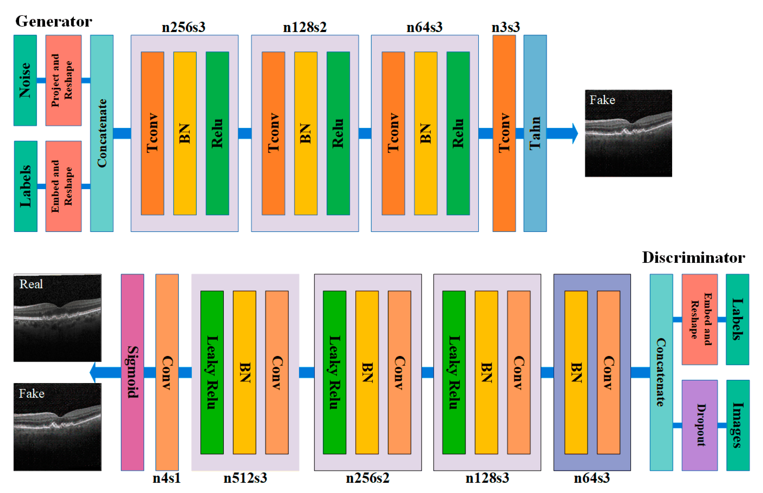
This paper reconstructs a 100-element random vector projection in the generator network as a 4 × 4 × 1024 array. Four convolution layers, three ReLU activation layers, and three batch normalization layers are added to the generated array to increase its dimensions to 256 × 256 × 3. For transposed convolutional layers, the filter size is 5 × 5, and the number of layer groups decreases in increments of 3, 2, 3, and 3. The last layer is the tanh layer. In the discriminator network, the input is a 256 × 256 × 3 picture. The final output prediction score is determined by four convolutional layers, three leaky ReLU activation layers, and three batch normalization layers. The discard probability of the discard layer in the network is set to 0.5, and noise is added randomly to the image via the dropout layer. The convolution layer has a 5 × 5 filter size. The number of layers is gradually reduced in steps 3, 3, 2, and 3. The leakage ReLU scale has been set to 0.2, and the output layer contains a sigmoid layer with a filter size of 44 and an output range of [0, 1]. Layer-to-layer structural interactions are illustrated in Figure 2 for the CGAN network component layers. Figure 2 shows a schematic of a Generative Adversarial Network (GAN), specifically a Conditional GAN (CGAN), which is a type of deep learning model that is used to generate data that are similar to some input data. It consists of two parts, a generator and a discriminator, that are trained simultaneously through adversarial processes. The figure demonstrates how the structure of each layer in the CGAN network contributes to the transformation of the input noise into a fake image that is indistinguishable from real images, and how the discriminator assesses these images. The notation ‘n’ refers to the number of feature maps in a layer, and ‘s’ refers to the stride of the convolutional layers. This process is part of training the GAN, where the generator learns to produce more realistic images while the discriminator becomes better at distinguishing between real and generated images. The end goal is for the generator to create images that are good enough to fool the discriminator into thinking they are real.

4. Model Experiment

4.1. Retinal Dataset

The OCT images of retinal illness used in the study are developed by Kermany [42]. The datasets generated and analyzed during the current study are available in the (Large Dataset of Labeled Optical Coherence Tomography (OCT) and Chest X-Ray Images) repository (https://data.mendeley.com/datasets/rscbjbr9sj/3, accessed on 2 June 2018).

The dataset contains 108,309 OCT image datasets with subfolders for CNV, DME, DRUSEN and NORMAL labels and is organized into two folders (training and testing). We selected 37,205 OCT photos of choroidal neovascularization (CNV), 8616 OCT images of age-related macular degeneration vitreous warts (DRUSEN), 11,348 OCT images of diabetic macular edema (DME), and 51,140 OCT images of normal eyes for training. This dataset is referred to as the real dataset.

The research has provided additional details about the real dataset used in this study. The selection of this dataset was based on its extensive coverage of various pathologies and sufficient sample size, ensuring the accuracy and generalizability of the model training. Additionally, detailed statistical information about the dataset, such as the number of images per disease type, image resolution, and quality, has been thoroughly assessed to ensure the validity and reliability of the study. Further enhancing the transparency of our research, our research also provides detailed information on data preprocessing and enhancement techniques used, which significantly impact the final performance of the model.

4.2. Experiment Results

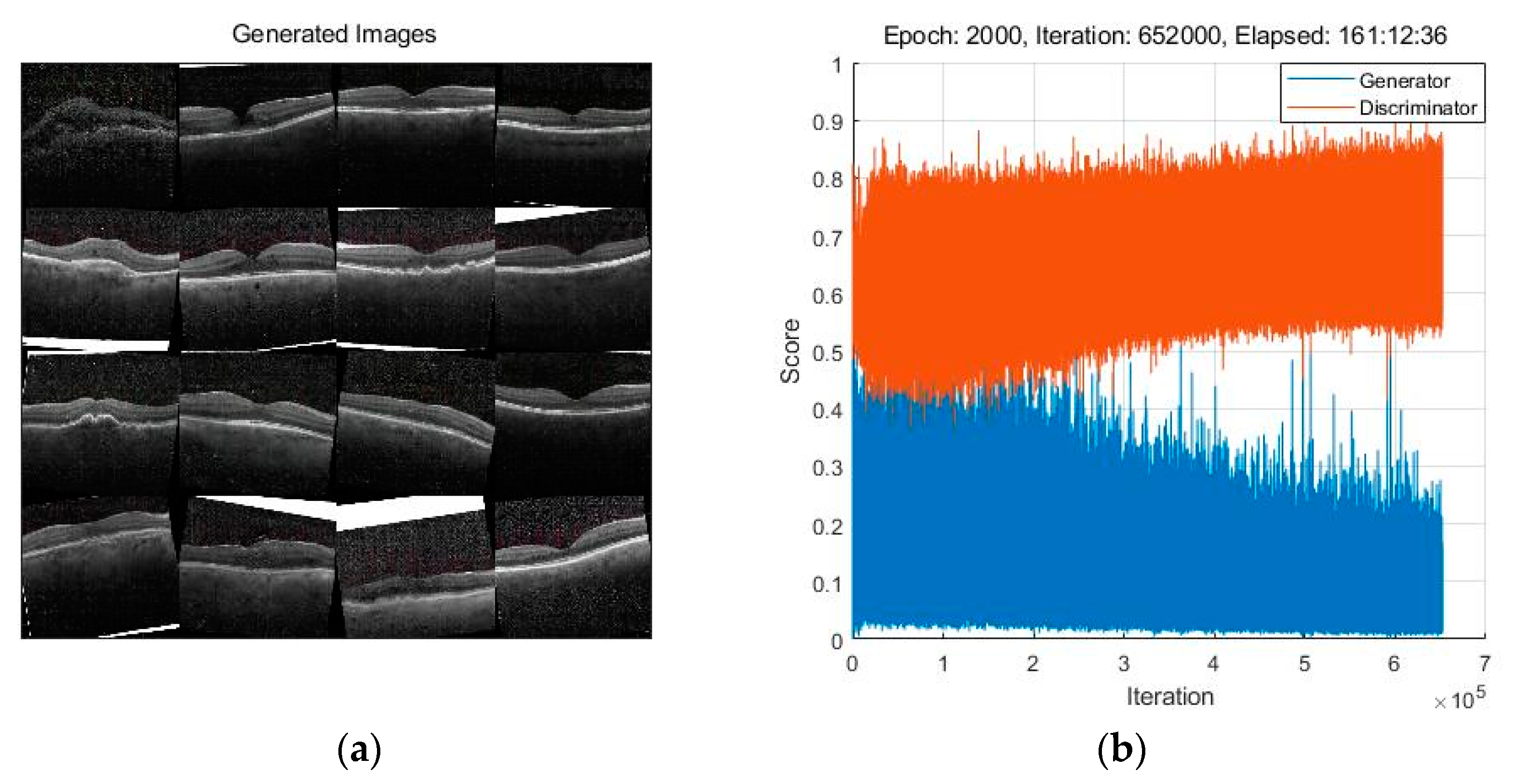
MATLAB 2022a is used for all software development for the experiments. Computer configurations, 12th Generation Intel Core i9-12900KS 5.5 GHz CPU and NVIDIA GeForce RTX 3090 Ti GPU with 10,752 CUDA units. Two thousand iterations are set for this experiment, and it took around 161 h to complete the training. Figure 3 depicts the modified CGAN [36] for training and sampling of images output.

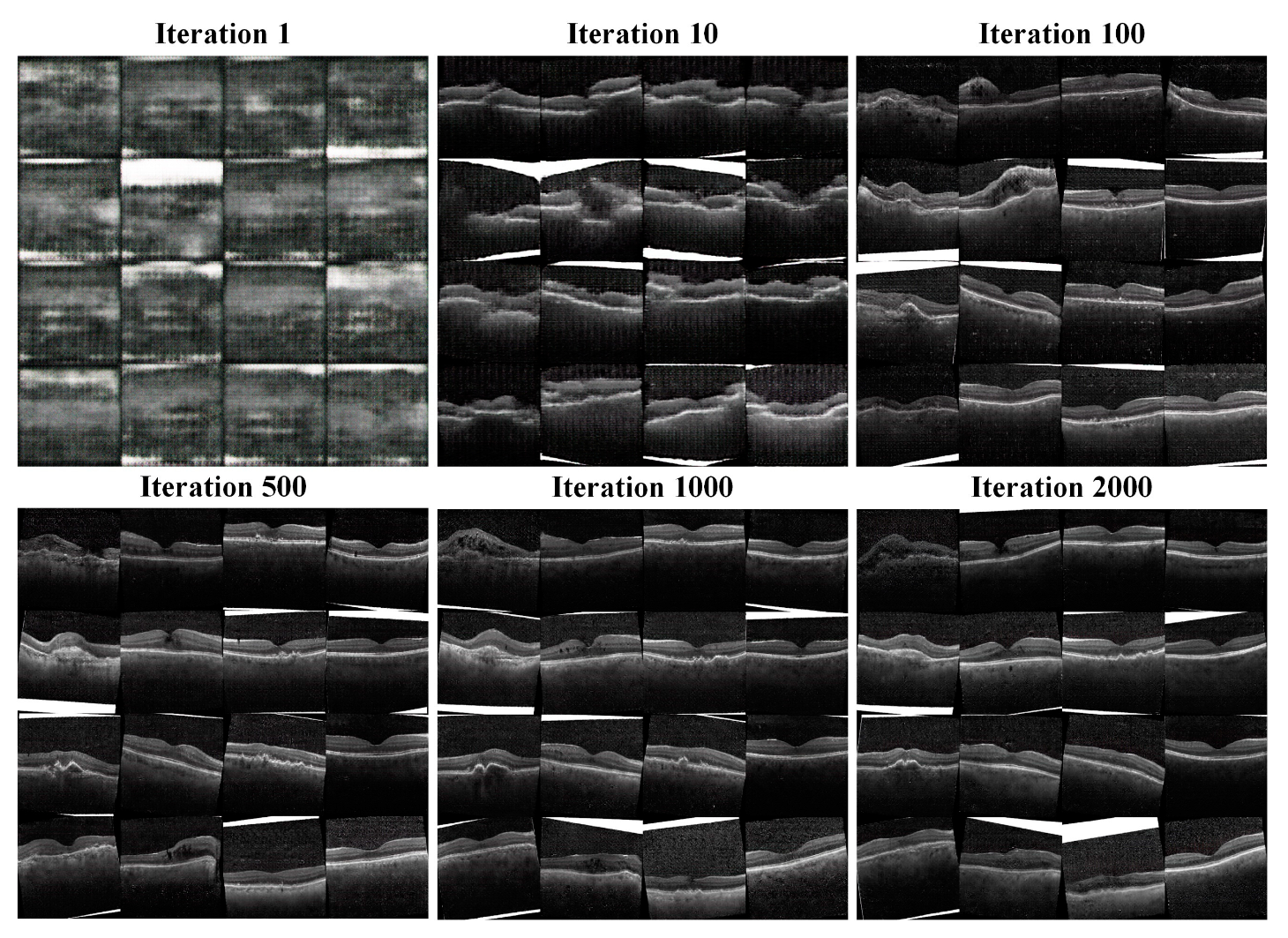
During training, randomized data enhancements such as random flips along the axis, different rotation angles, and randomly shifted pixels are introduced to increase the diversity of the data. Adam [43] is selected as the optimizer for training. In this study, the CGAN is suited for the gradient-based stochastic objective function optimization algorithm with a quicker processing performance than SGDM [44]. The training parameters are adjusted to obtain the optimal settings: mini batch size = 256, learn rate = 0.0002, gradient decay factor = 0.5. Of the samples, 70 percent are selected as the training set and 30 percent as the experiment set. Figure 4 depicts the modifications made to the synthetic OCT at the 1st, 10th, 100th, 1000th, 1500th, and 2000th iterations. It can be seen that as the number of iterations increases, the features of the image gradually become clearer. The feature image is progressively more complete and clear in 500 to 2000 iterations.

An array of specified labels and random vectors are fed into the trained CGAN network and then are converted to dimensional labels and fed through a generator to produce synthetic graphics on the GPU. A total of 102,400 OCTs are generated by four labels to create a synthetic dataset, and the real dataset is randomly combined with the synthetic dataset to produce a hybrid dataset, as shown in

Table 1. Dataset composition.

Dataset	Normal	Drusen	DME	CNV
Real Dataset [42]	51,140	8616	11,348	37,105
Generate Dataset	102,400	102,400	102,400	102,400
Hybrid Dataset	153,540	111,016	113,748	139,605

. Figure 5 compares the OCT images generated by CGAN for each class to real photos. It can be seen that the original dataset has been expanded and that the synthetic images used in the expansion have highly similar features to the real images.

5. CGAN Synthetic Image Quality Assessment

5.1. Transfer Learning-Based OCT Image Quality Assessment of Synthetic Retinal Diseases

5.1.1. Quality Assessment Models Based on Transfer Learning

Transfer learning is a crucial component of classification networks. As a technique for machine learning, it enables the utilization of previously trained weights for various tasks. Thus, we employ transfer learning principles to develop assessment tools.

The evaluation process is given below. AlexNet, VGGNet, DarkNet, Inception Net, ResNet, MobileNet, NasNet, ShuffleNet, GoogleNet, Squeezenet, Xception are adopted as pre-trained models, respectively. A dataset consisting of 70% training data and 30% experiment data was utilized. A test set from the real dataset containing 250 sheets for each category of retinal OCT illness was used.

The evaluation begins with pre-processing, where the input data are resize based on the size of the inputs to the pre-trained network. The input of the dataset into the 18 pre-trained models is the most crucial step in the system evaluation and diagnosis.

Eighteen deep-learning models are trained in this system using the retinal OCT hybrid dataset. With these models, we can validate the set to obtain a score for each model and prevent overfitting by utilizing a test set derived from the real dataset. The scoring measures enable us to determine the performance of the model and whether the model has received a high score. This indicates that the dataset employed by the model is of good quality, ultimately meaning that the images created by CGAN are sufficiently “realistic” to generate high-quality, highly usable synthetic retinal OCT images. The setups of models utilized for transfer learning are displayed in

Table 2. Model configuration.

Network	Input	Layer	Batch Size	Epoch	Learning Rate	Momentum	Optimizer	Time(Min)
AlexNet [45]	227 × 227 × 3	8	64	6	0.001	0.9	sgdm	32
Googlenet [46]	224 × 224 × 3	22	64	6	0.001	0.9	sgdm	46
ShuffleNet [47]	224 × 224 × 3	50	64	6	0.001	0.9	sgdm	89
SqueezeNet [48]	227 × 227 × 3	18	64	6	0.001	0.9	sgdm	25
Xception [49]	299 × 299 × 3	71	64	6	0.001	0.9	sgdm	264
MobileNet V2 [50]	224 × 224 × 3	53	64	6	0.001	0.9	sgdm	90
InceptionNet V3 [51]	299 × 299 × 3	48	64	6	0.001	0.9	sgdm	168
EfficientNet b0 [52]	224 × 224 × 3	82	64	6	0.001	0.9	sgdm	255
DenseNet201 [53]	224 × 224 × 3	201	64	6	0.001	0.9	sgdm	486
VGGNet16 [54]	224 × 224 × 3	16	64	6	0.001	0.9	sgdm	106
VGGNet19 [54]	224 × 224 × 3	19	64	6	0.001	0.9	sgdm	112
DarkNet19 [55]	256 × 256 × 3	19	64	6	0.001	0.9	sgdm	89
DarkNet53 [56]	256 × 256 × 3	23	64	6	0.001	0.9	sgdm	194
ResNet18 [57]	224 × 224 × 3	18	64	6	0.001	0.9	sgdm	50
ResNet50 [57]	224 × 224 × 3	50	64	6	0.001	0.9	sgdm	95
ResNet101 [57]	224 × 224 × 3	101	64	6	0.001	0.9	sgdm	150
Nasnet mobile [58]	224 × 224 × 3	-	64	6	0.001	0.9	sgdm	317
Nasnet large [58]	331 × 331 × 3	-	64	6	0.001	0.9	sgdm	3460

. In the study, we found that the deeper the layers, the longer the training time. Figure 6 illustrates the evaluation mechanism for generative graphs, which is essentially based on multiple transfer learning.

5.1.2. Experimental Result

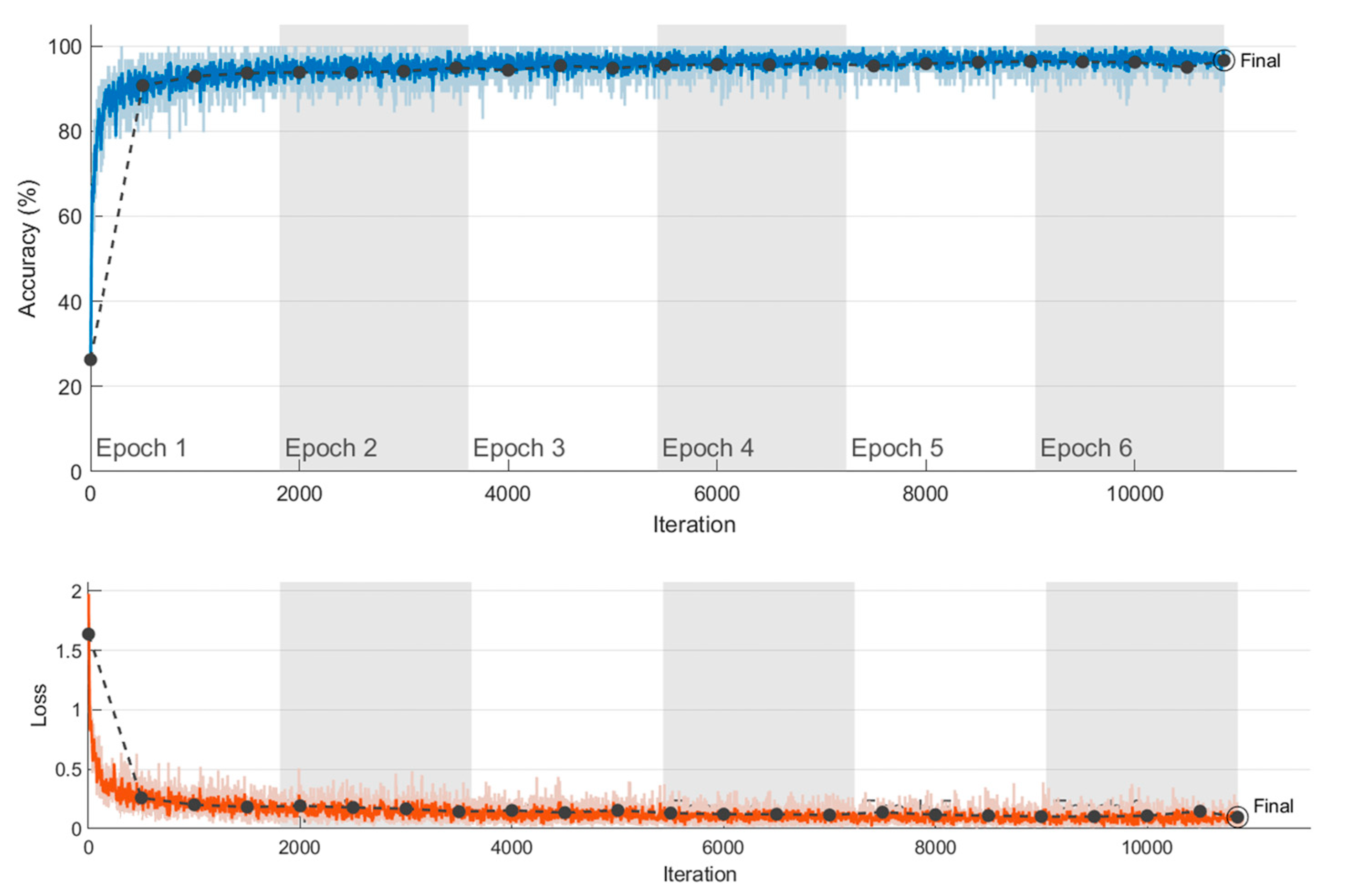
Figure 7 depicts the training plots of GoogleNet. The accuracy of the training set is shown with a blue label, the cross-entropy loss training set with an orange label, and all experiment sets with a black label (black dotted dashed line). Image normalization and 0.6 smoothings were performed to reveal the trend curve.

5.1.3. Accuracy and Assessment

Precision has a direct bearing on the evaluation of image quality. A confusion matrix was used to evaluate the performance of 18 models. The 18 models were evaluated based on the experiment set accuracy, the test set accuracy, and the recall balance [59]. The experiment set is used to determine the accuracy of the final result. Accuracy, Precision, Recall, F1 score are calculated by the following formula:

$$\mathrm{A}\mathrm{c}\mathrm{c}\mathrm{u}\mathrm{r}\mathrm{a}\mathrm{c}\mathrm{y}=\frac{\mathrm{T}\mathrm{P}+\mathrm{T}\mathrm{N}}{\left(\mathrm{T}\mathrm{P}+\mathrm{F}\mathrm{P}\right)+\left(\mathrm{T}\mathrm{N}+\mathrm{F}\mathrm{N}\right)}$$

(6)

$$\mathrm{P}\mathrm{r}\mathrm{e}\mathrm{c}\mathrm{i}\mathrm{s}\mathrm{i}\mathrm{o}\mathrm{n}=\frac{\mathrm{T}\mathrm{P}}{\mathrm{T}\mathrm{P}+\mathrm{F}\mathrm{P}}$$

(7)

$$\mathrm{R}\mathrm{e}\mathrm{c}\mathrm{a}\mathrm{l}\mathrm{l}=\frac{\mathrm{T}\mathrm{P}}{\mathrm{T}\mathrm{P}+\mathrm{F}\mathrm{N}}$$

(8)

$$\mathrm{F}1 \mathrm{S}\mathrm{c}\mathrm{o}\mathrm{r}\mathrm{e}=\frac{2\mathrm{T}\mathrm{P}}{\left(2\mathrm{T}\mathrm{P}+\mathrm{F}\mathrm{P}+\mathrm{F}\mathrm{N}\right)}$$

(9)

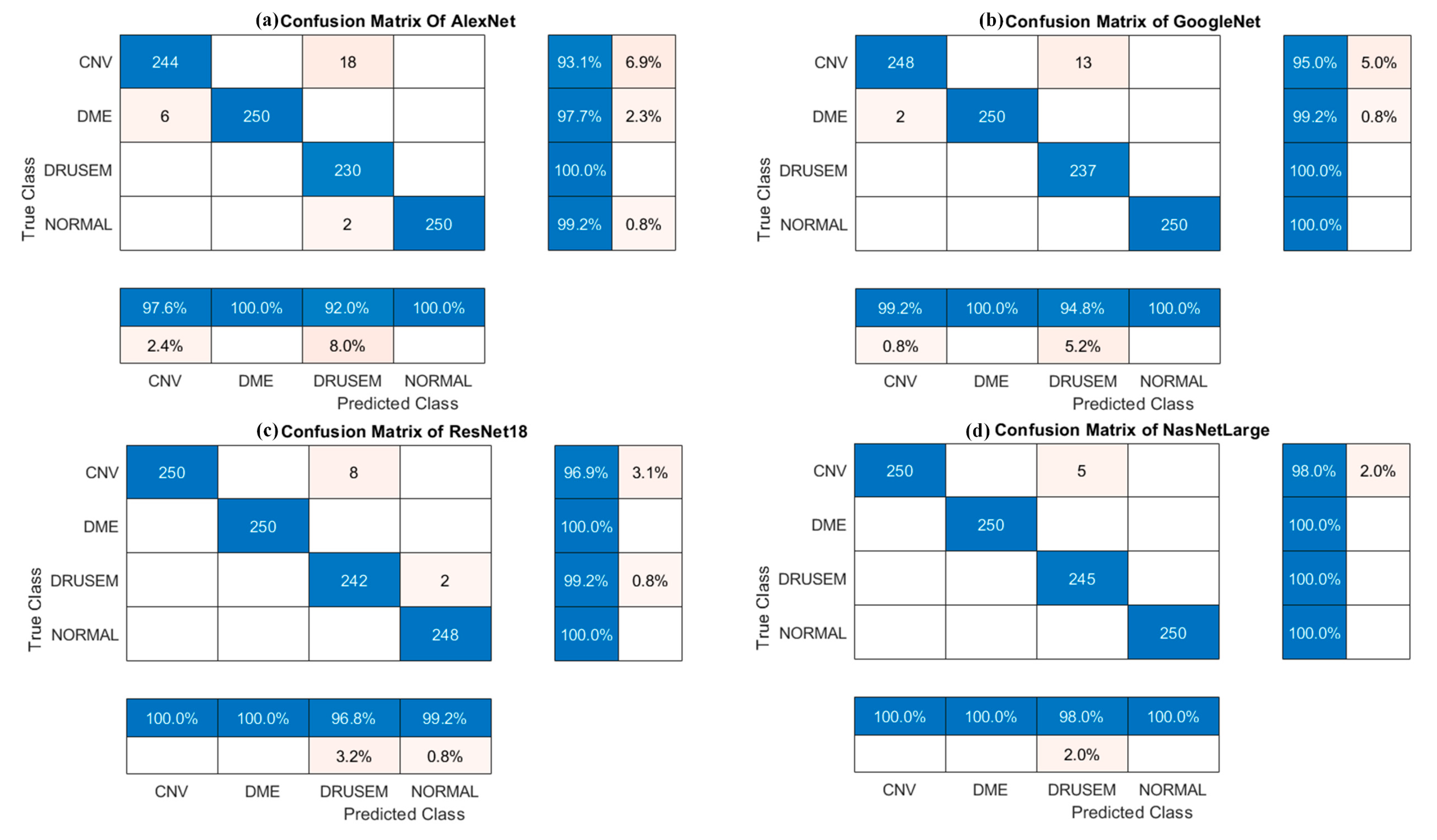
TP (True Positive) refers to a positive anticipated result and an actual positive outcome, whereas FP (False Positive) refers to a positive expected result and an actual negative result. TN (True Negative) is a pessimistic prediction and an actual negative result. FN (False Negative) is a predicted outcome that is negative, but the actual result is positive. FN (False Negative) refers to an anticipated negative consequence and an actual positive effect. Four confusion matrices of the different model are displayed in Figure 8. Images a–d are the confusion matrices for AlexNet, GoogleNet, ResNet18, and NasNetLarge, respectively. As the performance of the models improves, the confusion matrix reveals that the proportions of TP and TN steadily grow, converging towards the diagonal, while the ratios of FP and FN gradually decrease.

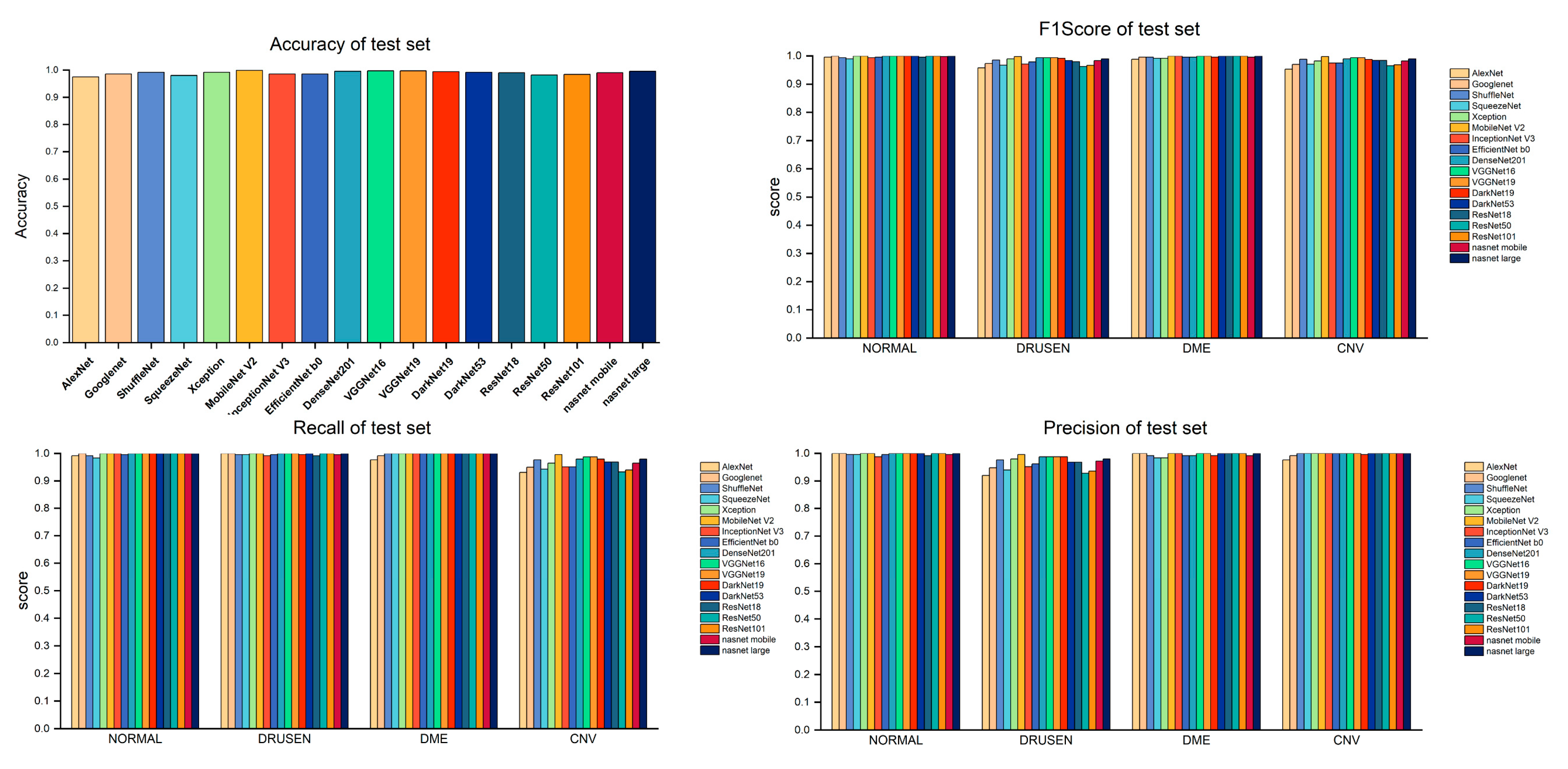
Figure 9 displays the four clock metrics measured using the experiment set for all 18 models. Alexnet still achieved an accuracy rate of 97.40%, even though it was the worst. The accuracy of the remaining models ranged from 98% to 100%. Eleven models reached at least 99% accuracy, representing 61% of all trained models. The accuracies of the experiment and test sets are displayed in

Table 3. Accuracy of the experiment and test sets of different models.

Model	Experiment Set	Test Set
AlexNet [46]	94.40%	97.40%
Googlenet [47]	96.59%	98.50%
ShuffleNet [48]	95.46%	99.10%
SqueezeNet [49]	92.93%	98.00%
Xception [50]	96.68%	99.10%
MobileNet V2 [50]	95.97%	99.90%
InceptionNet V3 [51]	97.53%	98.50%
EfficientNet b0 [52]	95.51%	98.50%
DenseNet201 [53]	97.70%	99.50%
VGGNet16 [54]	97.23%	99.70%
VGGNet19 [54]	97.48%	99.70%
DarkNet19 [55]	97.48%	99.40%
DarkNet53 [56]	97.72%	99.20%
ResNet18 [57]	97.23%	99.00%
ResNet50 [57]	97.25%	98.20%
ResNet101 [57]	97.52%	98.40%
NasNet mobile [58]	96.53%	99.00%
NasNet large [58]	98.24%	99.50%

. All 18 models with varying performances obtained extremely high levels of accuracy in the test set, with a variance of 3.84%. Due to the low quantity and high quality of photos in the experiment set, the difference in accuracy is only 2.50%. It is illustrated, therefore, from an accuracy perspective that the main determinant of the high accuracy of the 18 models is the training set used, showing that the CGAN-generated OCT images have distinct characteristics and properties similar to those of real OCT images.

Accuracy is dependent on the anticipated outcome and the proportion of positive samples that are accurate. The recall is based on the actual sample, which includes the correct proportion of positive samples. Figure 9 depicts the precision and recall rates for the four categories across the 18 models examined. The results are more even in NORMAL and DME. The recall rate in DRUSEN is significantly higher than the precision rate.

In contrast, the CNV demonstrated a lower recall rate and a higher precision rate, demonstrating a negative relationship between the two rates. NORMAL and DME achieve a highly desirable situation, and DRUSEN and CNV have a significant correlation. Nonetheless, the differences are minor. By calculating the F-value, a detailed and comprehensive evaluation can be obtained. The Fscore formula assigns distinct weights to the precision and recall rates. The formulas are displayed below:

$${\mathrm{F}}_{\mathrm{S}\mathrm{c}\mathrm{o}\mathrm{r}\mathrm{e}}=(1+{\mathsf{\beta }}^2)\frac{\mathrm{P}\mathrm{r}\mathrm{e}\mathrm{c}\mathrm{i}\mathrm{s}\mathrm{i}\mathrm{o}\mathrm{n}\times \mathrm{R}\mathrm{e}\mathrm{c}\mathrm{a}\mathrm{l}\mathrm{l}}{{\mathsf{\beta }}^2\cdot \mathrm{P}\mathrm{r}\mathrm{e}\mathrm{c}\mathrm{i}\mathrm{s}\mathrm{i}\mathrm{o}\mathrm{n}+\mathrm{R}\mathrm{e}\mathrm{c}\mathrm{a}\mathrm{l}\mathrm{l}}$$

(10)

where β = 1.

The F1 Score is a weighted average of the precision and recall that reflects the quality of the model. After reconciliation and averaging, the F1 Score is in optimal condition, as shown in Figure 9. The F1 Score ranges between 99.4% and 100% for NORMAL, 95.8% and 100% for DRUSEN, 99.2% and 100% for DME, and 95.3% and 100% for CNV. The accuracy, recall, and F1 Score statistics demonstrate that the model trained with the hybrid dataset is of the highest quality possible. Furthermore, it is demonstrated that the CGAN-generated images exhibit specific characteristics and properties similar to those of real OCT images.

5.2. OCT Image Quality Assessment of Synthetic Retinal Diseases Based on Interpretable Analysis Methods

5.2.1. Interpretable Analysis Method

Interpretable analysis techniques emphasize the display of pictures or convolutional layers, employing an intuitive visual perception to explain the behavior of the network [60]. Although deep learning is challenging for human understanding as a black box, interpretable analysis can be used to describe the logic of decision-making.

This study employs procedures that lend themselves to refined analysis (Grad-CAM [38], occlusion sensitivity [39], and LIME [40]). The degree of “realism” of the composite image is assessed by comparing the mapping features of the real image and the composite image in the classification network. Figure 10 illustrates the evaluation mechanism based on the interpretable analysis methodology.

5.2.2. Image Quality Assessment

Each visualization technique relates to a distinct function for image output production. In this section, Grad-CAM, occlusion sensitivity, and LIME methodologies are used for evaluation, respectively.

For example, the GoogleNet training model was evaluated by selecting eight OCTs, two of each category, including one real image and one synthetic image. Three visualization and analysis techniques are used for deep learning GoogleNet network decision-making behavior, using real and synthetic images for theoretical comparison.

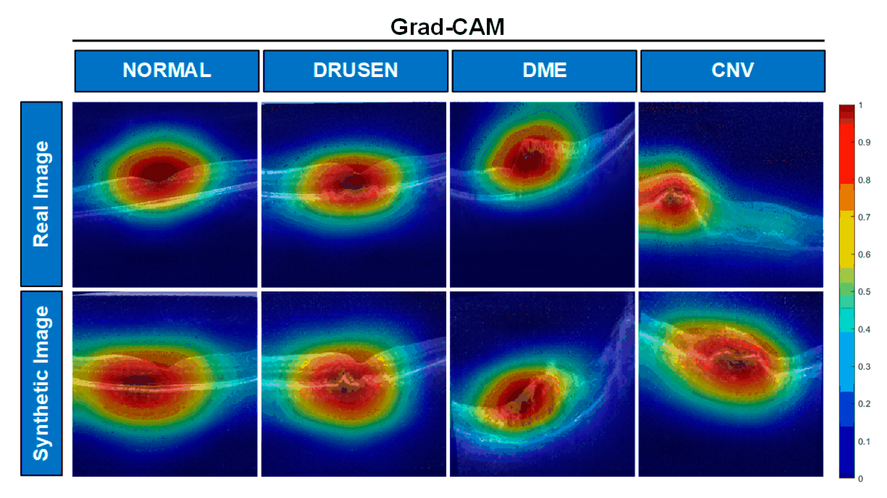
The Grad-CAM technique [38] is a gradient-based class activation heat map and extends the class activation mapping technique (CAM) [46]. CAM calculates scores for the gradient impact of convolutional features by determining those that play an essential role in classification. The stronger the reliance, the steeper the gradient. Figure 11 depicts a Grad-CAM plot of eight OCT images, with the genuine images [42] in the first row and the synthetic images in the second. The greater the score and gradient height, the darker the hue. The graphic depicts a color mapping with dark blue as the lowest value and red as the highest. Comparing real and synthetic images, the distribution of colors within the same category is comparable.

Occlusion sensitivity [40] is a heat map based on perturbations. The region is perturbed with masked blocks applied to the input data in this method. The occlusion sensitivity is attained by changing the masking blocks to isolate the components that play a significant role in categorization. To achieve the highest degree of occlusion sensitivity, the masks and Stride parameters must be set to precise levels for optimal masking sensitivity. Set MaskSize = 15 and Stride = 5. Figure 12 illustrates the occlusion sensitivity maps for each of the eight OCT images. The picture depicts how each component contributes to the classification. The larger the contribution, the darker the color. When comparing the genuine image to the composite image, the contribution of each component is comparable in images with similar compositions. The NORMAL and DRUSEN outside retinas exert the most influence on the DME and CNV, whereas the inner and outer retinas affect the CNV. Again, the largest contribution is typically centered in the inner and outer retinal deformations.

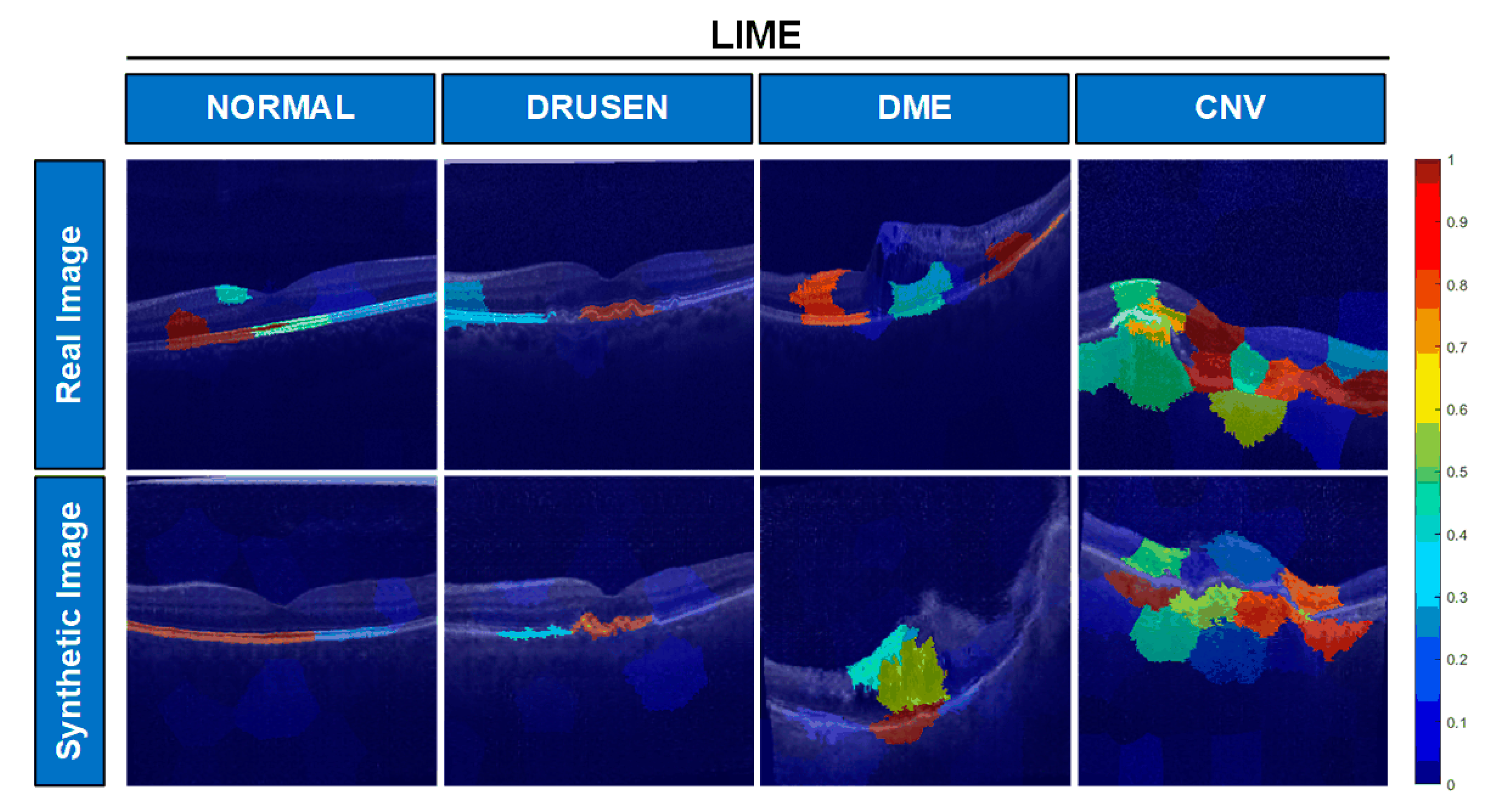
The LIME method [39] is a proxy model feature map that is perturbation-based. By approximating the classification behavior of the deep learning model to a smaller proxy model (regression model), the element scores of the picture are generated using the proxy model to determine the significance of each image component. Figure 13 displays the LIME maps for each of the eight OCT images. A regression tree is a simple model employed. The individual map area blocks show the relevance of the categorization of the photos. The darker red blocks are more significant. Comparing real and synthetic images, the categorization networks concentrate on similar areas, with NORMAL and DRUSEN focusing on the outside retinal area, DME and CNV being impacted by both the inner and outer retinal areas, CNV being affected by the inner retinal area over a greater area.

The results show that the synthetic images make similar contributions to the real images in the classification network, with an overall approximate distribution of score regions. It is illustrated that CGAN-synthesized OCT images have the main characteristics of real images.

6. Conclusions

This paper presents a modified CGAN to produce high-quality retinal OCT images, and two assessment methods are proposed to evaluate the quality of the synthetic images. The first evaluation method is based on 18 models with transfer learning, and calculations of accuracy, precision, recall, and F1 Sore parameters were carried out. In addition, an interpretable analytical method is based on three visualization techniques was used to comparing the contributions of the real and generated images to the classification model. Separate analyses were conducted on the classification network’s conclusions regarding the real and artificial images. Both evaluation techniques demonstrate that the quality of CGAN-generated OCT images of retinal disease is comparable to that of real OCT images of retinal disease. The generative OCT images from CGAN can be substituted for actual images. The primary drawback is the limited resolution of the generative images. Future study will focus on pre-processing and super-resolution of the images in order to enhance the resolution of CGAN generative images.

References

1. Laíns, I.; Wang, J.C.; Cui, Y.; Katz, R.; Vingopoulos, F.; Staurenghi, G.; Vavvas, D.G.; Miller, J.W.; Miller, J.B. Retinal applications of swept source optical coherence tomography (OCT) and optical coherence tomography angiography (OCTA). Prog. Retin. Eye Res. 2021, 84, 100951. [Google Scholar] [CrossRef] [PubMed]
2. Huang, D.; Swanson, E.A.; Lin, C.P.; Schuman, J.S.; Stinson, W.G.; Chang, W.; Hee, M.R.; Flotte, T.; Gregory, K.; Puliafito, C.A.; et al. Optical coherence tomography. Science 1991, 254, 1178–1181. [Google Scholar] [CrossRef] [PubMed]
3. Yang, Z.; Shang, J.; Liu, C.; Zhang, J.; Liang, Y. Identification of oral precancerous and cancerous tissue by swept source optical coherence tomography. Lasers Surg. Med. 2022, 54, 320–328. [Google Scholar] [CrossRef] [PubMed]
4. Kuranov, R.V.; Qiu, J.; McElroy, A.B.; Estrada, A.; Salvaggio, A.; Kiel, J.; Dunn, A.K.; Duong, T.Q.; Milner, T.E. Depth-resolved blood oxygen saturation measurement by dual-wavelength photothermal (DWP) optical coherence tomography. Biomed. Opt. Express 2011, 2, 491–504. [Google Scholar] [CrossRef]
5. Li, T.; Bo, W.; Hu, C.; Kang, H.; Liu, H.; Wang, K.; Fu, H. Applications of deep learning in fundus images: A review. Med. Image Anal. 2021, 69, 101971. [Google Scholar] [CrossRef] [PubMed]
6. Mitchell, P.; Liew, G.; Gopinath, B.; Wong, T.Y. Age-related macular degeneration. Lancet 2018, 392, 1147–1159. [Google Scholar] [CrossRef] [PubMed]
7. Grossniklaus, H.E.; Green, W.R. Choroidal neovascularization. Am. J. Ophthalmol. 2004, 137, 496–503. [Google Scholar] [CrossRef]
8. Bhagat, N.; Grigorian, R.A.; Tutela, A.; Zarbin, M.A. Diabetic macular edema: Pathogenesis and treatment. Surv. Ophthalmol. 2009, 54, 1–32. [Google Scholar] [CrossRef]
9. Uddin, S.; Khan, A.; Hossain, E.; Moni, M.A. Comparing different supervised machine learning algorithms for disease prediction. BMC Med. Inform. Decis. Mak. 2019, 19, 281. [Google Scholar] [CrossRef]
10. LeCun, Y.; Bengio, Y.; Hinton, G. Deep learning. Nature 2015, 521, 436–444. [Google Scholar] [CrossRef]
11. Guo, Y.; Liu, Y.; Oerlemans, A.; Lao, S.; Wu, S.; Lew, M.S. Deep learning for visual understanding: A review. Neurocomputing 2016, 187, 27–48. [Google Scholar] [CrossRef]
12. Shanthi, T.; Sabeenian, R.S. Modified Alexnet architecture for classification of diabetic retinopathy images. Comput. Electr. Eng. 2019, 76, 56–64. [Google Scholar] [CrossRef]
13. Subrahmanyeswara, R.B. Accurate leukocoria predictor based on deep VGG-net CNN technique. IET Image Process. 2020, 14, 2241–2248. [Google Scholar] [CrossRef]
14. Choudhry, Z.A.; Shahid, H.; Aziz, S.; Naqvi, S.Z.H.; Khan, M.U. DarkNet-19 Based Intelligent Diagnostic System for Ocular Diseases. Iran. J. Sci. Technol. Trans. Electr. Eng. 2022, 46, 959–970. [Google Scholar] [CrossRef]
15. Kamble, R.M.; Chan, G.C.Y.; Perdomo, O.; Kokare, M.; Gonzalez, F.A.; Muller, H.; Meriaudeau, F. Automated diabetic macular edema (DME) analysis using fine tuning with inception-resnet-v2 on OCT images. In Proceedings of the 2018 IEEE-EMBS Conference on Biomedical Engineering and Sciences (IECBES), Sarawak, Malaysia, 3–6 December 2018; IEEE: Piscataway, NJ, USA, 2018; pp. 442–446. [Google Scholar] [CrossRef]
16. Santos-Bustos, D.F.; Nguyen, B.M.; Espitia, H.E. Towards automated eye cancer classification via VGG and ResNet networks using transfer learning. Eng. Sci. Technol. Int. J. 2022, 2022, 101214. [Google Scholar] [CrossRef]
17. Abbas, Q.; Qureshi, I.; Ibrahim, M.E. An automatic detection and classification system of five stages for hypertensive retinopathy using semantic and instance segmentation in DenseNet architecture. Sensors 2021, 21, 6936. [Google Scholar] [CrossRef]
18. Ubaidah, I.D.W.S.; Fu’Adah, Y.; Sa’Idah, S.; Magdalena, R.; Wiratama, A.B.; Simanjuntak, R.B.J. Classification of Glaucoma in Fundus Images Using Convolutional Neural Network with MobileNet Architecture. In Proceedings of the 2022 1st International Conference on Information System & Information Technology (ICISIT), Yogyakarta, Indonesia, 27–28 July 2022; IEEE: Piscataway, NJ, USA, 2022; pp. 198–203. [Google Scholar] [CrossRef]
19. Lee, J.; Kim, Y.K.; Park, K.H.; Jeoung, J.W. Diagnosing glaucoma with spectral-domain optical coherence tomography using deep learning classifier. J. Glaucoma 2020, 29, 287–294. [Google Scholar] [CrossRef]
20. Salma, A.; Bustamam, A.; Sarwinda, D. Diabetic Retinopathy Detection Using GoogleNet Architecture of Convolutional Neural Network through Fundus Images. Nusant. Sci. Technol. Proc. 2021, 2021, 1–6. [Google Scholar] [CrossRef]
21. Saleh, N.; Abdel Wahed, M.; Salaheldin, A.M. Transfer learning-based platform for detecting multi-classification retinal disorders using optical coherence tomography images. Int. J. Imaging Syst. Technol. 2022, 32, 740–752. [Google Scholar] [CrossRef]
22. Kermany, D.S.; Goldbaum, M.; Cai, W.; Valentim, C.C.S.; Liang, H.; Baxter, S.L.; McKeown, A.; Yang, G.; Wu, X.; Yan, F.; et al. Identifying medical diagnoses and treatable diseases by image-based deep learning. Cell 2018, 172, 1122–1131. [Google Scholar] [CrossRef]
23. Goddard, M. The EU General Data Protection Regulation (GDPR): European regulation that has a global impact. Int. J. Mark. Res. 2017, 59, 703–705. [Google Scholar] [CrossRef]
24. Kuwayama, S.; Ayatsuka, Y.; Yanagisono, D.; Uta, T.; Usui, H.; Kato, A.; Takase, N.; Ogura, Y.; Yasukawa, T. Automated detection of macular diseases by optical coherence tomography and artificial intelligence machine learning of optical coherence tomography images. J. Ophthalmol. 2019, 2019, 6319581. [Google Scholar] [CrossRef]
25. Goodfellow, I.; Pouget-Abadie, J.; Mirza, M.; Xu, B.; Warde-Farley, D.; Ozair, S.; Courville, A.; Bengio, Y. Generative adversarial networks. Commun. ACM 2020, 63, 139–144. [Google Scholar] [CrossRef]
26. Liu, Y.C.; Yang, H.H.; Huck Yang, C.H.; Huang, J.H.; Tian, M.; Morikawa, H.; Tsai, Y.C.J.; Tegner, J. Synthesizing new retinal symptom images by multiple generative models. In Proceedings of the 14th Asian Conference on Computer Vision, Perth, Australia, 2–6 December 2018; Springer: Berlin/Heidelberg, Germany, 2018; pp. 235–250. [Google Scholar] [CrossRef]
27. Yanagihara, R.T.; Lee, C.S.; Ting, D.S.W.; Lee, A.Y. Methodological challenges of deep learning in optical coherence tomography for retinal diseases: A review. Transl. Vis. Sci. Technol. 2020, 9, 11. [Google Scholar] [CrossRef] [PubMed]
28. Burlina, P.M.; Joshi, N.; Pacheco, K.D.; Liu, T.Y.A.; Bressler, N.M. Assessment of deep generative models for high-resolution synthetic retinal image generation of age-related macular degeneration. JAMA Ophthalmol. 2019, 137, 258–264. [Google Scholar] [CrossRef] [PubMed]
29. Zheng, R.; Liu, L.; Zhang, S.; Zheng, C.; Bunyak, F.; Xu, R.; Li, B.; Sun, M. Detection of exudates in fundus photographs with imbalanced learning using conditional generative adversarial network. Biomed. Opt. Express 2018, 9, 4863–4878. [Google Scholar] [CrossRef]
30. Tajmirriahi, M.; Kafieh, R.; Amini, Z.; Lakshminarayanan, V. A Dual-Discriminator Fourier Acquisitive GAN for Generating Retinal Optical Coherence Tomography Images. IEEE Trans. Instrum. Meas. 2022, 71, 5015708. [Google Scholar] [CrossRef]
31. Seo, J.; Kang, J.-S.; Park, G.-M. LFS-GAN: Lifelong Few-Shot Image Generation. In Proceedings of the IEEE/CVF International Conference on Computer Vision (ICCV), Paris, France, 2–3 October 2023. [Google Scholar] [CrossRef]
32. You, A.; Kim, J.K.; Ryu, I.H.; Yoo, T.K. Application of generative adversarial networks (GAN) for ophthalmology image domains: A survey. Eye Vis. 2022, 9, 6. [Google Scholar] [CrossRef]
33. Liu, S.; Hu, W.; Xu, F.; Chen, W.; Liu, J.; Yu, X.; Wang, Z.; Li, Z.; Li, Z.; Yang, X.; et al. Prediction of OCT images of short-term response to anti-VEGF treatment for diabetic macular edema using different generative adversarial networks. Photodiagn. Photodyn. Ther. 2023, 41, 103272. [Google Scholar] [CrossRef]
34. Yu, X.; Li, M.; Ge, C.; Shum, P.P.; Chen, J.; Liu, L. A generative adversarial network with multi-scale convolution and dilated convolution res-network for OCT retinal image despeckling. Biomed. Signal Process. Control 2023, 80, 104231. [Google Scholar] [CrossRef]
35. Khalifa, N.E.; Loey, M.; Mirjalili, S. A comprehensive survey of recent trends in deep learning for digital images augmentation. Artif. Intell. Rev. 2021, 2021, 2351–2377. [Google Scholar] [CrossRef] [PubMed]
36. Mirza, M.; Osindero, S. Conditional generative adversarial nets. arXiv 2014, arXiv:1411.1784. [Google Scholar] [CrossRef]
37. Weiss, K.; Khoshgoftaar, T.M.; Wang, D. A survey of transfer learning. J. Big Data 2016, 3, 9. [Google Scholar] [CrossRef]
38. Selvaraju, R.R.; Cogswell, M.; Das, A. Grad-cam: Visual explanations from deep networks via gradient-based localization. In Proceedings of the IEEE International Conference on Computer Vision, Venice, Italy, 22–29 October 2017; pp. 618–626. [Google Scholar] [CrossRef]
39. Zeiler, M.D.; Fergus, R. Visualizing and understanding convolutional networks. In Proceedings of the European Conference on Computer Vision, Zurich, Switzerland, 6–12 September 2014; Springer: Berlin/Heidelberg, Germany, 2014; pp. 818–833. [Google Scholar] [CrossRef]
40. Ribeiro, M.T.; Singh, S.; Guestrin, C. “Why should I trust you?” Explaining the predictions of any classifier. In Proceedings of the 22nd ACM SIGKDD International Conference on Knowledge Discovery and Data Mining, San Francisco, CA, USA, 13–17 August 2016; pp. 1135–1144. [Google Scholar] [CrossRef]
41. Singh, A.; Sengupta, S.; Lakshminarayanan, V. Explainable deep learning models in medical image analysis. J. Imaging 2020, 6, 52. [Google Scholar] [CrossRef] [PubMed]
42. Kermany, D.; Zhang, K.; Goldbaum, M. Large dataset of labeled optical coherence tomography (OCT) and chest x-ray images. Mendeley Data 2018, 3, 10.17632. [Google Scholar] [CrossRef]
43. Kingma, D.P.; Ba, J. Adam: A method for stochastic optimization. arXiv 2014, arXiv:1412.6980. [Google Scholar] [CrossRef]
44. Qian, N. On the momentum term in gradient descent learning algorithms. Neural Netw. 1999, 12, 145–151. [Google Scholar] [CrossRef]
45. Krizhevsky, A.; Sutskever, I.; Hinton, G.E. Imagenet classification with deep convolutional neural networks. Commun. ACM 2017, 60, 84–90. [Google Scholar] [CrossRef]
46. Szegedy, C.; Liu, W.; Jia, Y.; Sermanet, P.; Reed, S.; Anguelov, D.; Erhan, D.; Vanhoucke, V.; Rabinovich, A.; Liu, W.; et al. Going deeper with convolutions. In Proceedings of the IEEE Conference on Computer Vision and Pattern Recognition, Boston, MA, USA, 7–12 June 2015; pp. 1–9. [Google Scholar] [CrossRef]
47. Zhang, X.; Zhou, X.; Lin, M.; Sun, J. Shufflenet: An extremely efficient convolutional neural network for mobile devices. In Proceedings of the IEEE Conference on Computer Vision and Pattern Recognition, Salt Lake City, UT, USA, 18–23 June 2018; pp. 6848–6856. [Google Scholar] [CrossRef]
48. Iandola, F.N.; Han, S.; Moskewicz, M.W.; Ashraf, K.; Dally, W.J.; Keutzer, K. SqueezeNet: AlexNet-level accuracy with 50x fewer parameters and <0.5 MB model size. arXiv 2016, arXiv:1602.07360. [Google Scholar] [CrossRef]
49. Chollet, F. Xception: Deep learning with depthwise separable convolutions. In Proceedings of the IEEE Conference on Computer Vision and Pattern Recognition, Honolulu, HI, USA, 21–26 July 2017; pp. 1251–1258. [Google Scholar] [CrossRef]
50. Sandler, M.; Howard, A.; Zhu, M.; Zhmoginov, A.; Chen, L. Mobilenetv2, Inverted residuals and linear bottlenecks. In Proceedings of the IEEE Conference on Computer Vision and Pattern Recognition, Salt Lake City, UT, USA, 18–23 June 2018; pp. 4510–4520. [Google Scholar] [CrossRef]
51. Szegedy, C.; Vanhoucke, V.; Ioffe, S.; Shlens, J.; Wojna, Z. Rethinking the inception architecture for computer vision. In Proceedings of the IEEE Conference on Computer Vision and Pattern Recognition, Las Vegas, NV, USA, 27–30 June 2016; pp. 2818–2826. [Google Scholar] [CrossRef]
52. Tan, M.; Le, Q. Efficientnet: Rethinking model scaling for convolutional neural networks. In Proceedings of the International Conference on Machine Learning (PMLR), Long Beach, CA, USA, 9–15 June 2019; pp. 6105–6114. [Google Scholar]
53. Huang, G.; Liu, Z.; Van Der Maaten, L.; Weinberger, K.Q. Densely connected convolutional networks. In Proceedings of the IEEE Conference on Computer Vision and Pattern Recognition, Honolulu, HI, USA, 21–26 July 2017; pp. 4700–4708. [Google Scholar]
54. Simonyan, K.; Zisserman, A. Very deep convolutional networks for large-scale image recognition. arXiv 2014, arXiv:1409.1556. [Google Scholar] [CrossRef]
55. Redmon, J.; Farhadi, A. YOLO9000, better, faster, stronger. In Proceedings of the IEEE Conference on Computer Vision and Pattern Recognition, Honolulu, HI, USA, 21–26 July 2017; pp. 7263–7271. [Google Scholar] [CrossRef]
56. Redmon, J.; Farhadi, A. Yolov3, An incremental improvement. arXiv 2018, arXiv:1804.02767. [Google Scholar] [CrossRef]
57. He, K.; Zhang, X.; Ren, S.; Sun, J. Deep residual learning for image recognition. In Proceedings of the IEEE Conference on Computer Vision and Pattern Recognition, Las Vegas, NV, USA, 27–30 June 2016; pp. 770–778. [Google Scholar]
58. Zoph, B.; Vasudevan, V.; Shlens, J.; Le, Q.V. Learning transferable architectures for scalable image recognition. In Proceedings of the IEEE Conference on Computer Vision and Pattern Recognition, Salt Lake City, UT, USA, 18–23 June 2018; pp. 8697–8710. [Google Scholar] [CrossRef]
59. Goutte, C.; Gaussier, E. A probabilistic interpretation of precision, recall and F-score, with implication for evaluation. In Proceedings of the 27th European Conference on Information Retrieval, Santiago de Compostela, Spain, 21–23 March 2005; Springer: Berlin/Heidelberg, Germany, 2005; pp. 345–359. [Google Scholar] [CrossRef]
60. Zhou, B.; Khosla, A.; Lapedriza, A.; Oliva, A.; Torralba, A. Learning deep features for discriminative localization. In Proceedings of the IEEE Conference on Computer Vision and Pattern Recognition, Las Vegas, NV, USA, 27–30 June 2016; pp. 2921–2929. [Google Scholar] [CrossRef]
Figure 1. Conditional generative adversarial network.
Processes 12 00182 g001
Figure 2. The modified CGAN layers structure.
Processes 12 00182 g002
Figure 3. The modified CGAN for training and sampling of images output. (a) Iterative sampling map; (b) Training process.
Processes 12 00182 g003
Figure 4. Sample plots for different iterations of the modified CGAN model.
Processes 12 00182 g004
Figure 5. Comparison of synthetic OCT images with real images.
Processes 12 00182 g005
Figure 6. Transfer learning-based assessment mechanism.
Processes 12 00182 g006
Figure 7. Model training process.
Processes 12 00182 g007
Figure 8. Confusion matrices of different models.
Processes 12 00182 g008
Figure 9. Performance measurements of eight models.
Processes 12 00182 g009
Figure 10. Assessment mechanism based on interpretable analysis methods.
Processes 12 00182 g010
Figure 11. Comparison of real and synthetic images Grad-CAM.
Processes 12 00182 g011
Figure 12. Comparison of occlusion sensitivity between real and synthetic images.
Processes 12 00182 g012
Figure 13. Real and synthetic image LIME comparison.
Processes 12 00182 g013