A Novel Nonlinear Filter-Based Robust Adaptive Control Method for a Class of Nonlinear Discrete-Time Systems

Abstract

This paper introduces an innovative adaptive control approach utilizing a nonlinear filter for a specific subset of nonlinear discrete-time systems, considering the presence of both input and output noise. The system can be transformed into a nonlinear autoregressive moving average with exogenous inputs (NARMAX) model. The concept of discrete Nussbaum gain is introduced to address the theoretical constraint associated with unknown directions of feed-forward or control gains, and the extended adaptive tuning sequence is introduced to facilitate the acceleration of parameter updating. In the case of no noise, asymptotical output tracking and global stability are achieved with the adaptive control. Further, in the presence of input noise and output noise, a novel nonlinear filter is designed to generate a more accurate filtered output, which improves the control system’s ability to adapt and track accurately. Finally, examples are provided to showcase the effectiveness and precision of the method.

1. Introduction

In past years, a substantial amount of research has been devoted to advancing the field of adaptive control for continuous-time nonlinear systems. Numerous industrial processes exhibit nonlinear behavior, and various methods have been developed for identifying nonlinear systems, which can be applied to input nonlinear systems, output nonlinear systems, and systems with both input and output nonlinearities [1,2,3,4].

This effort has entailed a thorough investigation into the backstepping design method, broadening its scope to cater to the needs of nonlinear continuous-time systems. Such systems can be efficiently converted into output feedback forms or parametric strict-feedback forms [5,6,7,8]. The results of these inquiries have also been expanded to encompass the domain of continuous Multiple-Input Multiple-Output (MIMO) systems [9,10,11]. Despite the considerable strides made toward comprehending adaptive control in continuous systems, it is noteworthy that the discrete counterparts of these findings have not received commensurate exploration.

In groundbreaking studies [12,13], progressive developments in adaptive control schemes for linear discrete-time models have been achieved. These outcomes have been expanded to address the challenges posed by discrete Multiple-Input Multiple-Output (MIMO) systems featuring nonparametric uncertainty [14]. It is worth noting, however, that within a substantial body of literature on adaptive control, a prerequisite for a priori knowledge is the awareness of control gains’ signs, referred to as control directions.

There are numerous methods commonly used for nonlinear system identification, including the joint two-stage least squares method proposed by Hu et al. [15]; based on recursive identification methods, advancements have been made with the introduction of the recursive least squares sub-algorithm and the gradient stochastic sub-algorithm. These techniques are specifically designed for parameter estimation and fractional-order estimation, respectively. Paper [16] proposes a projection identification algorithm and stochastic gradient identification algorithm for Hammerstein nonlinear systems. Additionally, the Newton recursive and Newton iterative identification algorithms derived in the study enhance the convergence speed of the stochastic gradient algorithm. In order to address the computational complexity associated with signal modeling involving a large number of feature parameters, a parameter separation approach based on the distinct characteristics of the signals being modeled is proposed. To achieve high precision performance while reducing complexity, a gradient search method is employed [17], and two iterative sub-algorithms based on multi-innovation gradient (MIGI) are introduced. Then, a novel approach, known as the layered forgetting factor stochastic gradient algorithm, based on extended Kalman filtering, is introduced for the estimation of unknown states, parameters, and fractional orders [18].

In recent years, to address the prevalent issue of data loss in industrial processes, a novel approach has been introduced [19]. This approach combines auxiliary models and particle filters to accurately estimate missing outputs. Specifically, for a specific class of nonlinear systems, such as bilinear systems, which are prone to irregular missing data, two unbiased parameter estimation methods are proposed. The parameter estimation problem of controllable autoregressive moving average (ARMA) systems has been investigated using the maximum likelihood multi-innovation stochastic gradient algorithm [20], resulting in a substantial enhancement in computational efficiency. Wang et al. [21] focus on the parameter estimation problem in fractional-order nonlinear systems with autoregressive noise. By minimizing two criterion functions, a two-stage gradient-based iterative (2S-GI) algorithm was developed to address this challenge. The 2S-GI algorithm effectively reduces computational complexity while enhancing the accuracy of system identification. By introducing the U-model based control approach [22], the efficiency and generality of the control system design have been significantly improved. The approach presented in [23,24] utilizes a combination of the least squares algorithm and an observer-based parameter estimation algorithm to estimate the parameter matrices and states of state space systems with limited output availability. The reconstructed states are employed in accurate parameter estimation. In the research in [25,26], the focus lies on exploring recursive estimation algorithms that utilize the modified extended Kalman filter for Wiener nonlinear systems experiencing both process noise and measurement noise. The primary objective is to accurately estimate the parameters associated with the linear subsystem. In the context of parameter estimation for an input nonlinear controlled autoregressive moving average system with variable-gain nonlinearity, this study introduces an appropriate switching function to establish an analytical representation of variable-gain nonlinearity. Furthermore, it develops two estimation algorithms based on auxiliary models [27]: a modified extended stochastic gradient algorithm with a forgetting factor and a recursive extended least-squares algorithm.

In order to achieve a more seamless integration of the universal output feedback method with the Nussbaum gain method [28,29,30], a specially designed controller adjustment rule is implemented to update the Nussbaum gain. This innovative approach [31] successfully resolves the challenge of controlling the direction position. The presented control scheme, utilizing the multi-innovation stochastic gradient algorithm, offers a self-correcting capability, enabling the attainment of virtual optimal control. Notably, this approach both ensures closed-loop stability in the system and delivers remarkable improvements in performance. Ding Feng et al. [32,33,34,35] have made significant contributions to the field of nonlinear system adaptive control. Their research focuses on vital theoretical concepts in system identification, including auxiliary model identification principles, multi-innovation identification theory, and hierarchical identification principles. They have successfully validated the effectiveness of least squares and multi-innovation least squares parameter estimation algorithms, extending their application to diverse systems with colored noise. Furthermore, they have proposed an adaptive solution specifically tailored for dual-rate nonlinear systems, addressing the limitations imposed by hardware constraints on output sampling rates. Xu Ling et al. [36,37] focus on the problem of parameter estimation in nonlinear models. They apply the gradient recursion algorithm and utilize dynamic data windows to enhance estimation accuracy, providing valuable insights for subsequent research in this area. This method is designed to achieve highly accurate parameter estimation, making a substantial contribution to enhancing the precision of parameter estimation techniques.

In an effort to overcome this theoretical constraint, a significant contribution was made in [38], where the discrete Nussbaum gain was initially introduced to establish a globally stable adaptive control framework even when control directions are unknown. Subsequently, the discrete Nussbaum gain has been systematically applied in the adaptive control of nonlinear discrete-time systems, taking forms such as NARMAX, output-feedback, and strict-feedback [39,40,41,42,43].

Conversely, the discrete-time backstepping approach was initially presented in [44] and subsequently extended in later studies [45,46,47] to achieve robust adaptive control. However, when the control gains are not known, the effectiveness of discrete backstepping is compromised. To solve this problem, approaches with an n-step ahead predictor were created for n-th order output-feedback or strict-feedback nonlinear systems [48]. But the presence of prediction errors can lead to instability in systems of this nature. An augmented error, combining the prediction errors and the tracking error, is thus introduced.

In an attempt to extend the nonlinear adaptive control results, this paper focuses on investigating adaptive tracking in a specific category of nonlinear discrete-time systems, incorporating input feed-forward and output feedback mechanisms. In the adaptive control framework applied to these nonlinear systems, the input feed-forward links can not only avoid the predictions of future outputs, but can also speed up the response time to enhance the stability of nonlinear systems. However, we find that the difficulty lies in unknown feed-forward gain, associated with the first subsystem state. Lacking knowledge of the gain’s sign makes it unattainable to deduce the updating direction for parameter estimation. Taking the same idea of discrete Nussbaum gain into the updating law and introducing an extended adaptive tuning factor into the update law, a recently introduced adaptive control approach is used for systems of this nature in the absence of noise. The assurance of boundedness for all closed-loop signals is accompanied by the accomplishment of asymptotical output tracking.

In addition, the existence of input and output noise within systems may lead to a considerable degradation in the tracking performance of adaptive control. According to the Kalman filter [49,50,51,52], a novel nonlinear filter is proposed, by designing the corresponding time update and measurement update equations. Thus, a novel nonlinear filter-based adaptive control method is developed to obtain good robustness.

The rest of the paper is organized as follows. The system representation and transformation are shown in Section 2. In Section 3, without disturbance, an adaptive control scheme is proposed, and the corresponding stability analysis is conducted. A novel nonlinear filter-based adaptive control method, in the presence of external disturbances, is proposed in Section 4. Illustrative examples are shown in Section 5. Finally, conclusions are drawn in Section 6.

2. System Representation and Transformation

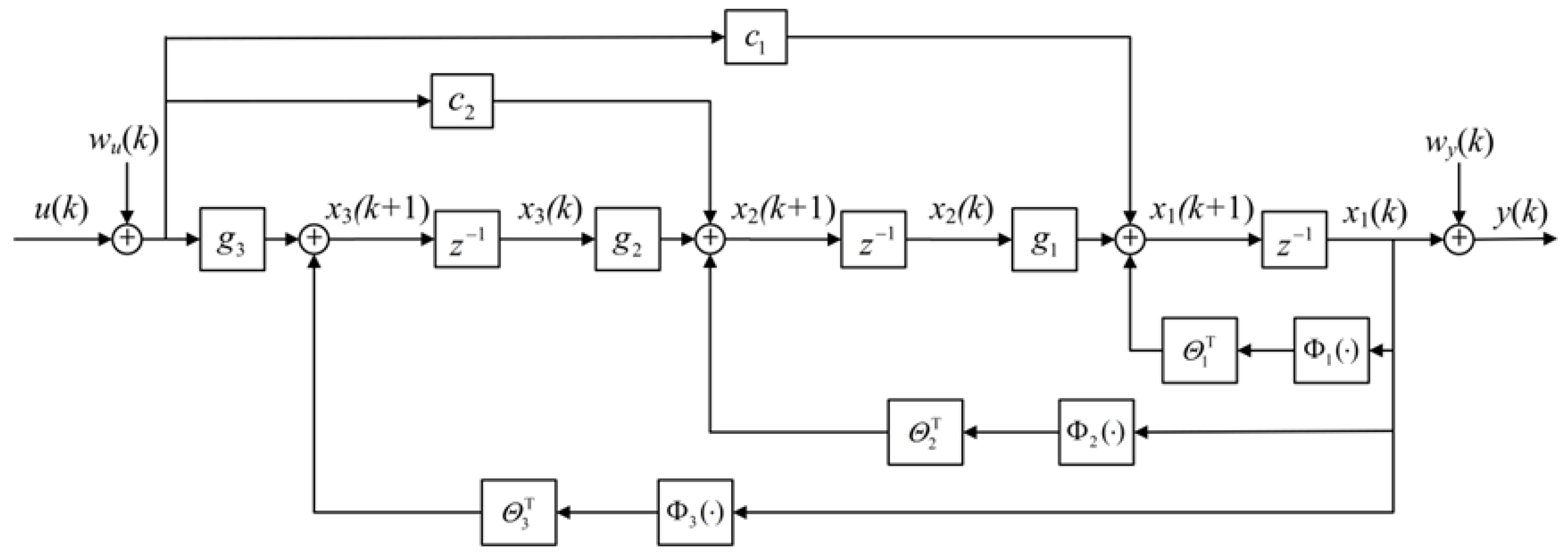
2.1. System Representation

Consider nonlinear SISO discrete-time systems in the following input feed-forward and output feedback form:

$$\left\{\begin{array}{l}{x}_1(k+1)={\Theta }_1^{\mathrm{T}}{\mathrm{\Phi }}_1(x_1(k))+g_1{x}_2(k)+c_1\left(u(k)+w_u(k)\right),\\ x_2(k+1)={\Theta }_2^{\mathrm{T}}{\mathrm{\Phi }}_2(x_1(k))+g_2{x}_3(k)+c_2\left(u(k)+w_u(k)\right),\\ \hspace{0.33em}\hspace{0.33em}\hspace{0.33em}\hspace{0.33em}\hspace{0.33em}⋮\\ x_{n-1}(k+1)={\Theta }_{n-1}^{\mathrm{T}}{\mathrm{\Phi }}_{n-1}(x_1(k))+g_{n-1}{x}_n(k)+c_{n-1}\left(u(k)+w_u(k)\right),\\ x_n(k+1)={\Theta }_n^{\mathrm{T}}{\mathrm{\Phi }}_n(x_1(k))+g_n\left(u(k)+w_u(k)\right),\\ y(k)=x_1(k)+w_y(k)\end{array}\right.$$

(1)

where ${\Theta }_i\in R^{q_i}$ are unknown parameter vectors, and ${\mathrm{\Phi }}_i(·)\hspace{0.33em}\hspace{0.33em}:\hspace{0.33em}\hspace{0.33em}R\to R^{q_i}$ are known nonlinear vector functions, $g_i\in R$ are unknown control gains, $c_i\in R$ are unknown feed-forward gains, $x_i(k)\in R$ are system states, and $n\ge 1$ is system order. Output $y(k)\in R$ consists of two parts: the first subsystem state $x_1(k)$ and the output noise $w_y(k)$. This proves that the name of the output feedback form is correct. The terms $w_u(k)$ represents the input noise. We assume that the input noise and output noise are affected by some known constants, i.e., $\left|w_y(k)\right|\le {\overline{w}}_y$, $\left|w_u(k)\right|\le {\overline{w}}_u$.

If the feed-forward gains equal zero, i.e., $c_1=\cdots =c_{n-1}=0$, this kind of system becomes the output feedback form suitable for the no noise case, as studied in [41]. The name “input feed-forward and output feedback” is deduced using block diagram in Figure 1, which, except for the unit delay operators, contains both feed-forward and feedback paths. In the theory of adaptive control, the input feed-forward links in nonlinear models avoid the predictions of future outputs or future states. In practice, the input feed-forward links improve the response speed and thus enhance the stability of nonlinear systems.

Assumption 1.

The nonlinear vectors  ${\mathrm{\Phi }}_i(·)$ are Lipschitz functions, i.e.,  $‖{\mathrm{\Phi }}_i({\xi }_1)-{\mathrm{\Phi }}_i({\xi }_2)‖\le L_i\left|{\xi }_1-{\xi }_2\right|$, $\forall {\xi }_1,\hspace{0.33em}{\xi }_2\in R,\hspace{0.33em}\hspace{0.33em}1\le i\le n$, where  $L_i$ is the Lipschitz coefficient. The control gains  $g_i\ne 0$ and the feed-forward gains  $c_i\ne 0.$

In presence of input noise and output noise, the objective of this paper is to design an adaptive control input $u(k)$ so that the output $y(k)$ tracks a bounded reference trajectory $y_a(k)$, and all the signals in the closed-loop system are bounded.

2.2. System Transformation

By introducing a state transformation ${\epsilon }_i(k)=x_i(k)·{\displaystyle {\prod }_{j=0}^{i-1}{g}_j}$ with $g_0=1$, the nonlinear system model of Equation (1) can be rewritten:

$$\left\{\begin{array}{l}{\epsilon }_1(k+1)={\Theta }_f^{\mathrm{T}}{\mathrm{\Phi }}_{f1}({\epsilon }_1(k))+{\epsilon }_2(k)+d_1\left(u(k)+w_u(k)\right),\\ {\epsilon }_2(k+1)={\Theta }_f^{\mathrm{T}}{\mathrm{\Phi }}_{f2}({\epsilon }_1(k))+{\epsilon }_3(k)+d_2\left(u(k)+w_u(k)\right),\\ \hspace{0.33em}⋮\\ {\epsilon }_{n-1}(k+1)={\Theta }_f^{\mathrm{T}}{\mathrm{\Phi }}_{f(n-1)}({\epsilon }_1(k))+{\epsilon }_n(k)+d_{n-1}\left(u(k)+w_u(k)\right),\\ {\epsilon }_n(k+1)={\Theta }_f^{\mathrm{T}}{\mathrm{\Phi }}_{fn}({\epsilon }_1(k))+d_n\left(u(k)+w_u(k)\right),\\ y(k)={\epsilon }_1(k)+w_y(k),\end{array}\right.$$

(2)

where

$$\begin{array}{l}{\Theta }_f={\left[{\Theta }_{f1}^{\mathrm{T}},\hspace{0.33em}\dots ,\hspace{0.33em}{\Theta }_{fn}^{\mathrm{T}}\right]}^{\mathrm{T}},\hspace{0.33em}\hspace{0.33em}\hspace{0.33em}\hspace{0.33em}\hspace{0.33em}{\Theta }_{fi}={\Theta }_i·{\displaystyle {\prod }_{j=0}^{i-1}{g}_j},\hspace{0.33em}\hspace{0.33em}\hspace{0.33em}{\mathrm{\Phi }}_{fi}={\left[0^{\mathrm{T}},\hspace{0.33em}{\mathrm{\Phi }}_i^{\mathrm{T}}(·),\hspace{0.33em}{0}^{\mathrm{T}}\right]}^{\mathrm{T}},\hspace{0.33em}\hspace{0.33em}\hspace{0.33em}\\ d_n={\displaystyle {\prod }_{j=0}^n{g}_j},\hspace{0.33em}\hspace{0.33em}\hspace{0.33em}{d}_i=c_i·{\displaystyle {\prod }_{j=0}^{i-1}{g}_j},\hspace{0.33em}\hspace{0.33em}\hspace{0.33em}i=1\hspace{0.33em},\hspace{0.33em}2,\hspace{0.33em}\dots ,\hspace{0.33em}n-1.\end{array}$$

(3)

3. Adaptive Control Design without Disturbance

3.1. Adaptive Control and Parameter Estimation

The adaptive control scheme is considered in the no noise case, i.e., $w_y(k)=0$, $w_u(k)=0$. If there is no input noise and no output noise, by iteratively substituting and combining all the equations in (2) together, the following system equations can be obtained:

$$y(k+n)={\Theta }_f^{\mathrm{T}}{\displaystyle \sum _{i=1}^n{\mathrm{\Phi }}_{fi}(y(k+n-i))}+{\displaystyle \sum _{i=1}^n{d}_{i}u(k+n-i)}.$$

(4)

At epoch $k+1$, the no noise output is obtained:

$$y(k+1)={\Theta }_f^{\mathrm{T}}{\displaystyle \sum _{i=1}^n{\mathrm{\Phi }}_{fi}(y(k-i+1))}+d_{1}u(k)+{\displaystyle \sum _{i=2}^n{d}_{i}u(k-i+1)}$$

(5)

Since $d_1=c_1{g}_0\ne 0$, we can get

$$\begin{array}{l}\psi (k)={\displaystyle \sum _{i=1}^n{\mathrm{\Phi }}_{fi}(y(k-i+1))},\hspace{0.33em}\hspace{0.33em}\hspace{0.33em}{\Theta }_{fd}=d_1^{-1}{\Theta }_f,\hspace{0.33em}\hspace{0.33em}\hspace{0.33em}{d}_f=d_1^{-1}·{\left[d_2,\hspace{0.33em}\dots ,\hspace{0.33em}{d}_n\right]}^{\mathrm{T}},\\ u_f(k)={\left[u(k-1),\hspace{0.33em}u(k-2),\hspace{0.33em}\dots ,\hspace{0.33em}u(k-n+1)\right]}^{\mathrm{T}}.\end{array}$$

Thus, yielding

$$\begin{array}{l}e(k+1)=y(k+1)-y_a(k+1)\\ \hspace{0.33em}\hspace{0.33em}\hspace{0.33em}\hspace{0.33em}\hspace{0.33em}\hspace{0.33em}\hspace{0.33em}\hspace{0.33em}\hspace{0.33em}=d_1·({\Theta }_{fd}^{\mathrm{T}}·\psi (k)+u(k)+d_f^{\mathrm{T}}·u_f(k)-d_1^{-1}{y}_a(k+1)).\end{array}$$

(6)

It is evident that the tracking error $e(k+1)$ can be reduced to zero by appropriately selecting $u(k)$

$$u(k)=-{\Theta }_{fd}^{\mathrm{T}}·\psi (k)-d_f^{\mathrm{T}}·u_f(k)+d_1^{-1}{y}_a(k+1).$$

(7)

However, due to the unknown parameters in nonlinear systems, replacing the unknown terms with their recursive estimates produces the following formula:

$$u(k)=-{\widehat{\Theta }}_{fd}^{\mathrm{T}}(k)·\psi (k)-{\widehat{d}}_f^{\mathrm{T}}(k)·u_f(k)+{\widehat{d}}_I(k)·y_a(k+1).$$

(8)

where ${\widehat{\Theta }}_{fd}^{\mathrm{T}}(k)$, ${\widehat{d}}_f^{\mathrm{T}}(k)$ and ${\widehat{d}}_I(k)$ are the estimates of ${\Theta }_{fd}^{\mathrm{T}}$, $d_f^{\mathrm{T}}$ and $d_1^{-1}$. Then, Equations (5)–(8), $e(k+1)$ can be obtained:

$$\begin{array}{l}e(k+1)=y(k+1)-y_a(k+1)\\ \hspace{0.33em}\hspace{0.33em}\hspace{0.33em}\hspace{0.33em}\hspace{0.33em}\hspace{0.33em}\hspace{0.33em}\hspace{0.33em}\hspace{0.33em}=d_1·\left(-{\tilde{\Theta }}_{fd}^{\mathrm{T}}(k)·\psi (k)-{\tilde{d}}_f^{\mathrm{T}}(k)·u_f(k)+{\tilde{d}}_I(k)·y_a(k+1)\right).\end{array}$$

(9)

where ${\tilde{\Theta }}_{fd}(k)$, ${\tilde{d}}_f(k)$ and ${\tilde{d}}_I(k)$ can be defined as

$${\tilde{\Theta }}_{fd}(k)={\widehat{\Theta }}_{fd}(k)-{\Theta }_{fd},\hspace{0.33em}\hspace{0.33em}\hspace{0.33em}{\tilde{d}}_f(k)={\widehat{d}}_f(k)-d_f,\hspace{0.33em}\hspace{0.33em}\hspace{0.33em}{\tilde{d}}_I(k)={\widehat{d}}_I(k)-d_1^{-1}.$$

(10)

In Equation (9), there is an unknown feedforward gain $d_1$, making recursive parameter estimation challenging without prior knowledge of $d_1$, and determining the update direction of parameter estimation is a challenge.

Therefore, to address this limitation, the discrete Nussbaum gain [38] is introduced. According to [38], the discrete Nussbaum gain $N(p(k))$ can be described as

$$N(p(k))=p_s(k)·s_N(p(k)),\hspace{0.33em}\hspace{0.33em}\hspace{0.33em}{p}_s(k)=\underset{k^{\prime }\le k}{\sup }\{p(k^{\prime })\},$$

(11)

where the term $s_N(p(k))$ is the sign function of the discrete nonlinear gain. Letting $Z(p(k))\triangleq {\displaystyle \sum _{k^{\prime }=0}^k\left(N(p(k^{\prime }))·\Delta p(k^{\prime })\right)}$ these lemmas are proved.

Lemma 1

([38]). Assuming $p_s(k)$ increases without bound, 

$$\underset{p_s(k)\ge {\tau }_0}{\sup }\frac{1}{p_s(k)}Z(p(k))=+\infty ,\hspace{0.33em}\hspace{0.33em}\hspace{0.33em}\underset{p_s(k)\ge {\tau }_0}{\inf }\frac{1}{p_s(k)}Z(p(k))=-\infty$$

(12)

Lemma 2

([38]). If $p_s(k)\le {\tau }_1$ , then $\left|Z(p(k))\right|\le {\tau }_2$, where ${\tau }_1$ and ${\tau }_2$ are some positive constants.

Therefore, by introducing the discrete Nussbaum gain to parameter estimation, we obtain the following update law:

$$\begin{array}{l}e(k)=y(k)-y_a(k),\hspace{0.33em}\hspace{0.33em}\upsilon (k)=\frac{e(k)}{G(k)},\\ {\widehat{\Theta }}_{fd}(k)={\widehat{\Theta }}_{fd}(k-1)+\frac{N(p(k))}{D(k)}\psi (k-1)\upsilon (k),\hspace{0.33em}\hspace{0.33em}\hspace{0.33em}{\widehat{\Theta }}_{fd}(0)=\mathbf{0},\\ {\widehat{d}}_f(k)={\widehat{d}}_f(k-1)+\frac{N(p(k))}{D(k)}{u}_f(k-1)\upsilon (k),\hspace{0.33em}\hspace{0.33em}\hspace{0.33em}{\widehat{d}}_f(0)=\mathbf{0},\\ {\widehat{d}}_I(k)={\widehat{d}}_I(k-1)-\frac{N(p(k))}{D(k)}{y}_a(k)\upsilon (k),\hspace{0.33em}\hspace{0.33em}\hspace{0.33em}{\widehat{d}}_I(0)=0,\\ G(k)=1+\left|N(p(k))\right|,\\ D(k)=G(k)·\left(1+{‖\psi (k-1)‖}^2+{‖u_f(k-1)‖}^2+y_a^2(k)+{\upsilon }^2(k)\right),\\ \Delta p(k)=p(k+1)-p(k)=\frac{G(k){\upsilon }^2(k)}{D(k)},\hspace{0.33em}\hspace{0.33em}\hspace{0.33em}p(0)=0,\end{array}$$

(13)

where $\upsilon (k)$ is augmented error, and $D(k)$ is normalization sequence. According to $p(k)$, we determine $0\le \Delta p(k)\le 1$ and $p(k)\ge 0$. Thus, sequence $p(k)$ is well satisfied.

In order to expedite the parameter updating process, a modified adaptive tuning factor $\gamma (k)$ is used to update the law. Based on the non-decreasing non-negative sequence $p(k)$, the tuning factor can be described by

$$\gamma (k)=4-3·{\mathrm{e}}^{-p(k)}$$

(14)

where $\gamma (k)$ is a monotonic increasing function of $p(k)$, and its values range from 1 to 4, i.e., $\gamma (k)\in [1,\hspace{0.33em}4]$. Thus, it is concluded that $\gamma (k)$ is a non-decreasing, bounded, and positive tuning factor. Then, by introducing the extended adaptive tuning factor $\gamma (k)$, the parameter updating process in (13) can be modified as follows:

$$\begin{array}{l}e(k)=y(k)-y_a(k),\hspace{0.33em}\hspace{0.33em}\gamma (k)=4-3·{\mathrm{e}}^{-p(k)},\hspace{0.33em}\hspace{0.33em}\upsilon (k)=\frac{\gamma (k)e(k)}{G(k)},\\ {\widehat{\Theta }}_{fd}(k)={\widehat{\Theta }}_{fd}(k-1)+\gamma (k)\frac{N(p(k))}{D(k)}\psi (k-1)\upsilon (k),\hspace{0.33em}\hspace{0.33em}\hspace{0.33em}{\widehat{\Theta }}_{fd}(0)=\mathbf{0},\\ {\widehat{d}}_f(k)={\widehat{d}}_f(k-1)+\gamma (k)\frac{N(p(k))}{D(k)}{u}_f(k-1)\upsilon (k),\hspace{0.33em}\hspace{0.33em}\hspace{0.33em}{\widehat{d}}_f(0)=\mathbf{0},\\ {\widehat{d}}_I(k)={\widehat{d}}_I(k-1)-\gamma (k)\frac{N(p(k))}{D(k)}{y}_a(k)\upsilon (k),\hspace{0.33em}\hspace{0.33em}\hspace{0.33em}{\widehat{d}}_I(0)=0,\\ G(k)=1+\left|N(p(k))\right|,\\ D(k)=G(k)·\left(1+{‖\psi (k-1)‖}^2+{‖u_f(k-1)‖}^2+y_a^2(k)+{\upsilon }^2(k)\right),\\ \Delta p(k)=p(k+1)-p(k)=\frac{G(k){\upsilon }^2(k)}{D(k)},\hspace{0.33em}\hspace{0.33em}\hspace{0.33em}p(0)=0.\end{array}$$

(15)

3.2. Asymptotic Tracking and Stability Analysis

Definition 1

([39]). Let $x_1(k)$ and  $x_2(k)$ be two discrete scalar or vector signals, $\forall k>k_0$ and $x_1(k)=O[x_2(k)]$, if positive constants $m_1$, $m_2$ and $k_0$ exist, to acquire $‖x_1(k)‖\le m_1{\max }_{k^{\prime }\le k}‖x_2(k^{\prime })‖+m_2$, $\forall k>k_0.$

Theorem 1.

For the nonlinear discrete-time system (1) under Assumption 1, consider the adaptive control (8) with recursive parameter update law (15). If there is no input noise and no output noise, all the closed-loop signals are bounded, and the tracking error  $e(k)$  will converge to zero.

Proof. 

From Equation (9), we obtain

$$\begin{array}{l}\gamma (k)·\left({\tilde{\Theta }}_{fd}^{\mathrm{T}}(k-1)·\psi (k-1)+{\tilde{d}}_f^{\mathrm{T}}(k-1)·u_f(k-1)-{\tilde{d}}_I(k-1)·y_a(k)\right)\\ =-\frac{1}{d_1}\gamma (k)e(k)=-\frac{1}{d_1}\upsilon (k)G(k).\end{array}$$

(16)

Define a non-negative function $V(k)$, we use

$$V(k)={‖{\tilde{\Theta }}_{fd}(k)‖}^2+{‖{\tilde{d}}_f(k)‖}^2+{\left({\tilde{d}}_I(k)\right)}^2.$$

(17)

The equation of $V(k)$ can be described as

$$\begin{array}{l}\Delta V(k)=V(k)-V(k-1)\\ ={\left[{\tilde{\Theta }}_{fd}(k)-{\tilde{\Theta }}_{fd}(k-1)\right]}^{\mathrm{T}}\left[{\tilde{\Theta }}_{fd}(k)-{\tilde{\Theta }}_{fd}(k-1)\right]+2{\tilde{\Theta }}_{fd}^{\mathrm{T}}(k-1)\left[{\tilde{\Theta }}_{fd}(k)-{\tilde{\Theta }}_{fd}(k-1)\right]\\ \hspace{0.33em}\hspace{0.33em}\hspace{0.33em}+2{\tilde{d}}_f^{\mathrm{T}}(k-1)\left[{\tilde{d}}_f(k)-{\tilde{d}}_f(k-1)\right]+{\left[{\tilde{d}}_f(k)-{\tilde{d}}_f(k-1)\right]}^{\mathrm{T}}\left[{\tilde{d}}_f(k)-{\tilde{d}}_f(k-1)\right]\\ \hspace{0.33em}\hspace{0.33em}\hspace{0.33em}+{\left({\tilde{d}}_I(k)-{\tilde{d}}_I(k-1)\right)}^2+2{\tilde{d}}_I(k-1)\left({\tilde{d}}_I(k)-{\tilde{d}}_I(k-1)\right)\\ =\frac{{\gamma }^2(k)N^2(p(k))·\left({\psi }^{\mathrm{T}}(k-1)·\psi (k-1)+u_f^{\mathrm{T}}(k-1)·u_f(k-1)+y_a^2(k)\right)}{D^2(k)}{\upsilon }^2(k)\\ \hspace{0.33em}\hspace{0.33em}\hspace{0.33em}+2\gamma (k)N(p(k))·\frac{{\tilde{\Theta }}_{fd}^{\mathrm{T}}(k-1)·\psi (k-1)+{\tilde{d}}_f^{\mathrm{T}}(k-1)·u_f(k-1)-{\tilde{d}}_I(k-1)·y_a(k)}{D(k)}\upsilon (k).\end{array}$$

(18)

According to (15) and (16), we obtain

$$\begin{array}{ll}\Delta V(k)& \le \frac{{\gamma }^2(k)G(k){\upsilon }^2(k)}{D(k)}+2N(p(k))·\frac{-1/d_1·\upsilon (k)G(k)}{D(k)}·\upsilon (k)\\ & \le 4^2·\Delta p(k)-\frac{2}{d_1}N(p(k))\Delta p(k).\end{array}$$

(19)

Then, we sum up the above equations to obtain

$$V(k)\le 16·p(k+1)+\left(-2/d_1\right)·\left({\displaystyle \sum _{k^{\prime }=0}^{k}N(p(k^{\prime }))\Delta p(k^{\prime })}\right).$$

(20)

Assuming that $p(k)$ is unbounded, due to $p(k)\ge 0$, $p_s(k)$ must increase without an upper bound. Hence, a constant $k_0$ must exist to give

$$\begin{array}{l}\Delta p(k)\le 1\le p_s(k),\hspace{0.33em}\hspace{0.33em}\hspace{0.33em}\forall k\ge k_0,\\ p(k+1)=p(k)+\Delta p(k)\le 2p_s(k),\hspace{0.33em}\hspace{0.33em}\hspace{0.33em}\forall k\ge k_0.\end{array}$$

(21)

Using Equations (20) and (21), the following inequality can be satisfied, $\forall k\ge k_0$,

$$\begin{array}{ll}0\le \frac{V(k)}{p_s(k)}& \le \frac{b}{p_s(k)}·\left({\displaystyle \sum _{k^{\prime }=0}^{k}N(p(k^{\prime }))\Delta p(k^{\prime })}\right)+\frac{16·p(k+1)}{p_s(k)}\\ & \le \frac{b}{p_s(k)}·Z(p(k))+32,\end{array}$$

(22)

where $b=-2/d_1$. According to Lemma 1, $\frac{1}{p_s(k)}Z(p(k))$ is unbounded because $p_s(k)$ increases without an upper bound, i.e.,

$$\underset{p_s(k)\ge 1}{\sup }\frac{1}{p_s(k)}Z(p(k))=+\infty ,\hspace{0.33em}\hspace{0.33em}\hspace{0.33em}\underset{p_s(k)\ge 1}{\inf }\frac{1}{p_s(k)}Z(p(k))=-\infty .$$

Therefore, it can be inferred that Equation (22) yields a contradiction, no matter if $b>0$ or $b<0$. As a result, $p(k)$ is bounded, as well as $p_s(k)$. Based on Lemma 2, $Z(p(k))$, $N(p(k))$, and $V(k)$ are bounded, this means that $G(k)$, ${\widehat{\Theta }}_{fd}(k)$, ${\widehat{d}}_f(k)$, and ${\widehat{d}}_I(k)$ are bounded.

Since $e(k)=y(k)-y_a(k)$ and the reference trajectory $y_a(k)$ is bounded, it is easy to obtain $y(k)=O[e(k)]$. And the Lipschitz condition of $\psi (·)$ indicates that

$$\psi (k-1)=O[e(k-1)]=O[e(k)],\hspace{0.33em}\hspace{0.33em}\hspace{0.33em}\hspace{0.33em}\hspace{0.33em}\psi (k)=O[e(k)].$$

(23)

Substituting $k=1$ into Equation (8), we have

$$u(1)=-{\widehat{\Theta }}_{fd}^{\mathrm{T}}(1)·\psi (1)-{\widehat{d}}_f^{\mathrm{T}}(1)·u_f(1)+{\widehat{d}}_I(1)·y_a(2).$$

(24)

where $u_f(1)={\left[u(0),\hspace{0.33em}u(-1),\hspace{0.33em}\dots ,\hspace{0.33em}u(-n+2)\right]}^{\mathrm{T}}=0$. From the boundedness of the parameter estimates from the above equation, we obtain $u(1)=O[e(1)]$. Considering that $k=2$, we can deduce that $u(2)=O[e(2)]$ and $u_f(2)=O[e(2)]$. Continuing the procedure, we can finally obtain $u(k)=O[e(k)]$ and $u_f(k)=O[e(k)]$.

Due to the augmented error $\upsilon (k)=\frac{\gamma (k)e(k)}{G(k)}=O[e(k)]$, it is not difficult to obtain the relationship between $D(k)$ and $e(k)$, i.e., $D(k)=O[e^2(k)]$. Since the term $p(k)$ is a non-decreasing non-negative sequence, the boundedness of $p(k)$ implies that

$$\Delta p(k)=\frac{G(k){\upsilon }^2(k)}{D(k)}=\frac{{\gamma }^2(k)e^2(k)}{D(k)G(k)}\to 0$$

(25)

Since $D(k)=O[e^2(k)]$ and the term $G(k)$ is bounded, according to the Lemma in [39], we conclude that $e(k)\to 0$. Then, the inputs and outputs in the nonlinear system are bounded. Further, for the system in Equation (2), in the no noise case, the states ${\epsilon }_i(k)$ are also bounded. This proves Theorem 1. □

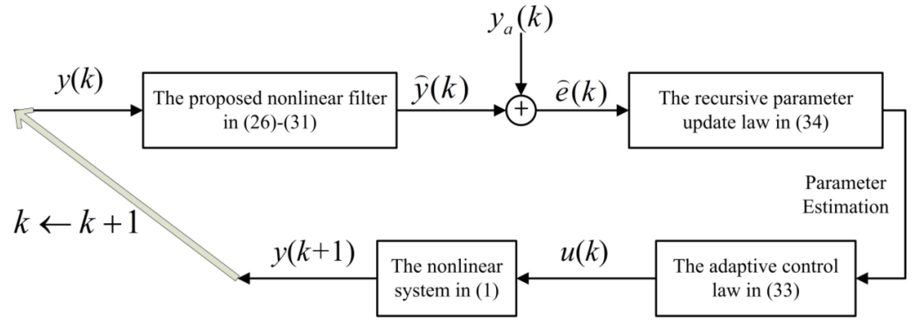
4. A Novel Nonlinear Filter-Based Adaptive Control Method in the Presence of Disturbances

In this section, a novel nonlinear filter is proposed for the nonlinear discrete-time systems in presence of input noise and output noise, i.e., $w_y(k)\ne 0$, and $w_u(k)\ne 0$. A more accurate filtered output is obtained via this nonlinear filter. Based on the theory of Kalman filter equations [50], an effective estimation technique is investigated for state estimation in nonlinear systems.

Generally, the equations for Kalman filters [50] are divided into two kinds: the time update equation plays a crucial role in advancing the current state and error covariance estimation and can be used to derive prior estimates for subsequent time steps. Conversely, the measurement update equations are introduced to assimilate a new measurement into an a priori estimate, leading to a more accurate posteriori estimate. According to the Kalman filter, the time update and measurement update equations can also be extended to our nonlinear filter, which is used as a state observer, in the presence of noise. For transformation (2) under Assumption 1, a nonlinear filter is designed.

The time update equations for the nonlinear filter are:

$$\left\{\begin{array}{l}{\epsilon }_1(k|k-1)={\widehat{\Theta }}_f^{\mathrm{T}}(k-1)·{\mathrm{\Phi }}_{f1}({\epsilon }_1(k-1|k-1))+{\epsilon }_2(k-1|k-1)+{\widehat{d}}_1(k-1)u(k-1),\\ {\epsilon }_2(k|k-1)={\widehat{\Theta }}_f^{\mathrm{T}}(k-1)·{\mathrm{\Phi }}_{f2}({\epsilon }_1(k-1|k-1))+{\epsilon }_3(k-1|k-1)+{\widehat{d}}_2(k-1)u(k-1),\\ \hspace{0.33em}\hspace{0.33em}\hspace{0.33em}\hspace{0.33em}\hspace{0.33em}\hspace{0.33em}⋮\\ {\epsilon }_n(k|k-1)={\widehat{\Theta }}_f^{\mathrm{T}}(k-1)·{\mathrm{\Phi }}_{fn}({\epsilon }_1(k-1|k-1))+{\widehat{d}}_n(k-1)u(k-1).\end{array}\right.$$

(26)

$$\left\{\begin{array}{l}{P}_{{\epsilon }_1}(k|k-1)={\widehat{\Theta }}_f^{\mathrm{T}}(k-1){\widehat{\Theta }}_f(k-1)·{\overline{L}}_1{}^2{P}_{{\epsilon }_1}(k-1|k-1)+P_{{\epsilon }_2}(k-1|k-1)+{\widehat{d}}_1{}^2{\overline{w}}_u{}^2,\\ P_{{\epsilon }_2}(k|k-1)={\widehat{\Theta }}_f^{\mathrm{T}}(k-1){\widehat{\Theta }}_f(k-1)·{\overline{L}}_2{}^2{P}_{{\epsilon }_1}(k-1|k-1)+P_{{\epsilon }_3}(k-1|k-1)+{\widehat{d}}_2{}^2{\overline{w}}_u{}^2,\\ \hspace{0.33em}\hspace{0.33em}\hspace{0.33em}\hspace{0.33em}\hspace{0.33em}\hspace{0.33em}⋮\\ P_{{\epsilon }_n}(k|k-1)={\widehat{\Theta }}_f^{\mathrm{T}}(k-1){\widehat{\Theta }}_f(k-1)·{\overline{L}}_n{}^2{P}_{{\epsilon }_1}(k-1|k-1)+{\widehat{d}}_n{}^2{\overline{w}}_u{}^2.\end{array}\right.$$

(27)

In Equations (26) and (27), the equations project forward the previous states ${\epsilon }_i(k-1|k-1)$ and error covariance estimates $P_{{\epsilon }_i}(k-1|k-1)$ to obtain priori estimates ${\epsilon }_i(k|k-1)$ and $P_{{\epsilon }_i}(k|k-1)$ for the current epoch k. The initial terms of the nonlinear filter are set to ${\epsilon }_i(0|0)=0$, $P_{{\epsilon }_i}(k|k-1)={10}^{-2}$. Meanwhile, the parameter estimates ${\widehat{\Theta }}_f^{\mathrm{T}}(k-1)$ and ${\widehat{d}}_i$ are given by the specific recursive parameter update law, which will be constructed and described below. In Equation (27), the terms ${\overline{L}}_i$, $i=1,\hspace{0.33em}\dots ,\hspace{0.33em}n$, are the minimum Lipschitz coefficients, which can be given using the numerical computation for the inequality $\frac{‖{\mathrm{\Phi }}_{fi}({\xi }_1)-{\mathrm{\Phi }}_{fi}({\xi }_2)‖}{\left|{\xi }_1-{\xi }_2\right|}\le {\overline{L}}_i=\min \{L_i\}$.

Next, the measurement update equations for our nonlinear filter must be designed. However, for the system transformation (2), the difficulty lies in the observation equation $y(k)={\epsilon }_1(k)+w_y(k)$, which only contains measurement values for the first subsystem state. This means that the measurement values for other states ${\epsilon }_i(k),\hspace{0.33em}\hspace{0.33em}i=2,\hspace{0.33em}\dots ,n$, are not available. For these other states, their a posteriori estimates are set to be equal to the corresponding priori estimates in the measurement update equations.

The measurement update equations for our nonlinear filter are:

$$K_{{\epsilon }_1}(k)=\frac{P_{{\epsilon }_1}(k|k-1)}{P_{{\epsilon }_1}(k|k-1)+\alpha ·{\overline{w}}_y{}^2},$$

(28)

$$\left\{\begin{array}{l}{\epsilon }_1(k|k)={\epsilon }_1(k|k-1)+K_{{\epsilon }_1}(k)·\left(y(k)-{\epsilon }_1(k|k-1)\right),\\ {\epsilon }_2(k|k)={\epsilon }_2(k|k-1),\\ \hspace{0.33em}\hspace{0.33em}\hspace{0.33em}\hspace{0.33em}\hspace{0.33em}\hspace{0.33em}\hspace{0.33em}⋮\\ {\epsilon }_n(k|k)={\epsilon }_n(k|k-1),\end{array}\right.$$

(29)

$$\left\{\begin{array}{l}{P}_{{\epsilon }_1}(k|k)=\left(1-K_{{\epsilon }_1}(k)\right)·P_{{\epsilon }_1}(k|k-1),\\ P_{{\epsilon }_2}(k|k)=P_{{\epsilon }_2}(k|k-1),\\ \hspace{0.33em}\hspace{0.33em}\hspace{0.33em}\hspace{0.33em}\hspace{0.33em}\hspace{0.33em}\hspace{0.33em}\hspace{0.33em}⋮\\ P_{{\epsilon }_n}(k|k)=P_{{\epsilon }_n}(k|k-1).\end{array}\right.$$

(30)

computing the nonlinear gain $K_{{\epsilon }_1}(k)$ for the first subsystem state. According to [49], this nonlinear gain is constructed based on the Kalman gain, and an adaptive factor $\alpha$ is designed to balance the output noise and the error covariance estimates. Then, the a posteriori estimates, as shown in Equation (29), can be generated. The final step is to calculate the a posteriori error covariance estimates via Equation (30). According to the design of an adaptive factor in [49], the term $\alpha$ can be chosen as

$$\alpha =\left\{\begin{array}{cc}1,\hfill & \hfill \mathrm{\Delta }\le r_0\\ \frac{r_0}{\mathrm{\Delta }}·{\left(\frac{r_1-\mathrm{\Delta }}{r_1-r_0}\right)}^2,\hfill & \hfill r_0<\mathrm{\Delta }\le r_1\\ 0,\hfill & \hfill \mathrm{\Delta }>r_1\end{array}\right.,$$

(31)

where $\Delta :=\frac{\left|y(k)-{\epsilon }_1(k|k-1)\right|}{\left|{\epsilon }_1(k|k-1)\right|}$ represents the relative output prediction error, and the terms $r_0$ and $\hspace{0.33em}{r}_1$ are constants, which are found to have the values $r_0=1$ and $r_1=3$.

Therefore, the nonlinear filtering algorithm in (26)–(31) is complete for state estimation in nonlinear systems. In order to obtain a more accurate filtered output, which is expected to track the reference trajectory, the output of the nonlinear filter is set to the first filtered subsystem state. From ${\epsilon }_1(k|k)$, the filtered output at epoch k is described as

$$\stackrel{⌢}{y}(k)={\epsilon }_1(k|k)$$

(32)

To develop the adaptive control of filtered output, we define

$$\stackrel{⌢}{e}(k)=\stackrel{⌢}{y}(k)-y_a(k),\hspace{0.33em}\hspace{0.33em}\stackrel{⌢}{\upsilon }(k)=\frac{\gamma (k)\stackrel{⌢}{e}(k)}{G(k)},\hspace{0.33em}\hspace{0.33em}\stackrel{⌢}{\psi }(k)={\displaystyle \sum _{i=1}^n{\mathrm{\Phi }}_{fi}(\stackrel{⌢}{y}(k-i+1))}.$$

Then, the adaptive control (8) can be rewritten as

$$u(k)=-{\widehat{\Theta }}_{fd}^{\mathrm{T}}(k)·\stackrel{⌢}{\psi }(k)-{\widehat{d}}_f^{\mathrm{T}}(k)·u_f(k)+{\widehat{d}}_I(k)·y_a(k+1)$$

(33)

In addition, the recursive parameter update law (15) must be modified. Using the dead zone method in [42], the term $l(k)$ is used to set the threshold for the updating process. Thus, the parameter update law using the filtered output can be shown as follows:

$$\begin{array}{l}\stackrel{⌢}{e}(k)=\stackrel{⌢}{y}(k)-y_a(k),\hspace{0.33em}\hspace{0.33em}\gamma (k)=4-3·{\mathrm{e}}^{-p(k)},\hspace{0.33em}\hspace{0.33em}\stackrel{⌢}{\upsilon }(k)=\frac{\gamma (k)\stackrel{⌢}{e}(k)}{G(k)},\\ {\widehat{\Theta }}_{fd}(k)={\widehat{\Theta }}_{fd}(k-1)+\gamma (k)l(k)\frac{N(p(k))}{D(k)}\stackrel{⌢}{\psi }(k-1)\stackrel{⌢}{\upsilon }(k),\hspace{0.33em}\hspace{0.33em}\hspace{0.33em}{\widehat{\Theta }}_{fd}(0)=\mathbf{0},\\ {\widehat{d}}_f(k)={\widehat{d}}_f(k-1)+\gamma (k)l(k)\frac{N(p(k))}{D(k)}{u}_f(k-1)\stackrel{⌢}{\upsilon }(k),\hspace{0.33em}\hspace{0.33em}\hspace{0.33em}{\widehat{d}}_f(0)=\mathbf{0},\\ {\widehat{d}}_I(k)={\widehat{d}}_I(k-1)-\gamma (k)l(k)\frac{N(p(k))}{D(k)}{y}_a(k)\stackrel{⌢}{\upsilon }(k),\hspace{0.33em}\hspace{0.33em}\hspace{0.33em}{\widehat{d}}_I(0)=0,\\ G(k)=1+\left|N(p(k))\right|,\\ D(k)=G(k)·\left(1+{‖\psi (k-1)‖}^2+{‖u_f(k-1)‖}^2+y_a^2(k)+{\stackrel{⌢}{\upsilon }}^2(k)\right),\\ \Delta p(k)=p(k+1)-p(k)=\frac{l(k)G(k){\stackrel{⌢}{\upsilon }}^2(k)}{D(k)},\hspace{0.33em}\hspace{0.33em}\hspace{0.33em}p(0)=0,\\ {\widehat{d}}_1(k)={\widehat{d}}_I{}^{-1}(k),\hspace{0.33em}\hspace{0.33em}\hspace{0.33em}{\left[{\widehat{d}}_2(k),\hspace{0.33em}\dots ,{\widehat{d}}_n(k)\right]}^{\mathrm{T}}={\widehat{d}}_1(k)·{\widehat{d}}_f(k),\hspace{0.33em}\hspace{0.33em}\hspace{0.33em}{\widehat{\Theta }}_f(k)={\widehat{d}}_1(k)·{\widehat{\Theta }}_{fd}(k),\\ l(k)=\left\{\begin{array}{c}\hspace{0.33em}1,\hspace{0.33em}\hspace{0.33em}\hspace{0.33em}\hspace{0.33em}if\hspace{0.33em}\hspace{0.33em}\left|\upsilon (k)\right|>\sigma ,\\ 0,\hspace{0.33em}\hspace{0.33em}\hspace{0.33em}\hspace{0.33em}\hspace{0.33em}\hspace{0.33em}\hspace{0.33em}\hspace{0.33em}\hspace{0.33em}\hspace{0.33em}o\mathrm{T}hers.\end{array}\right.\end{array}$$

(34)

where $\sigma$ is the threshold value determined by the designer. Using the nonlinear filtering algorithm in (26)–(31) and applying the adaptive control (33) with parameter update law (34) gives a complete nonlinear filter-based robust adaptive control method. The adaptive nonlinear filtering proposed in this paper is very preliminary, and further theoretical and practical studies are needed. A flowchart of the robust adaptive control scheme, according to nonlinear filter, is depicted in Figure 2.

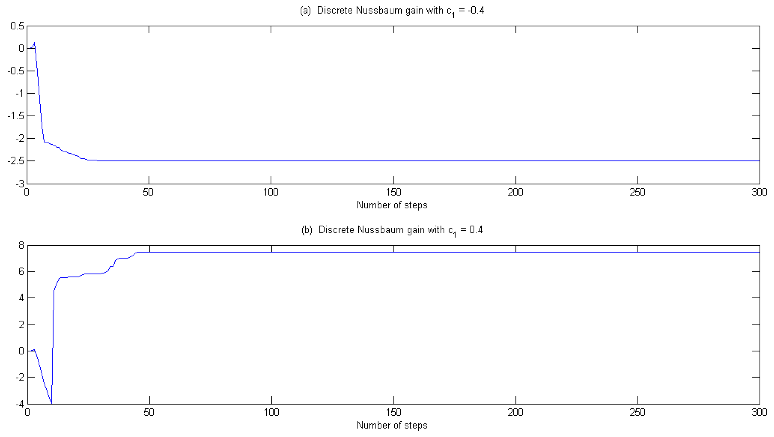
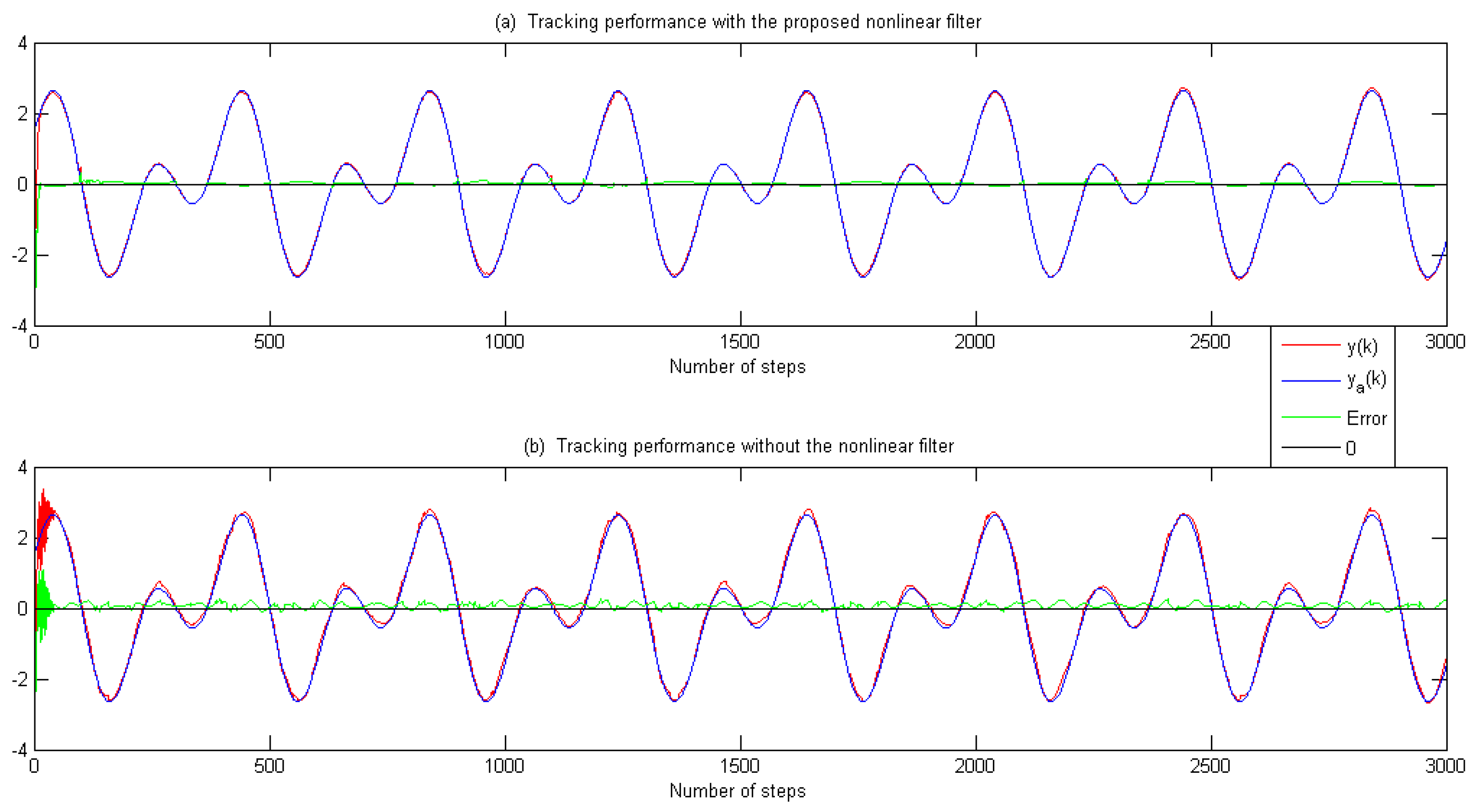
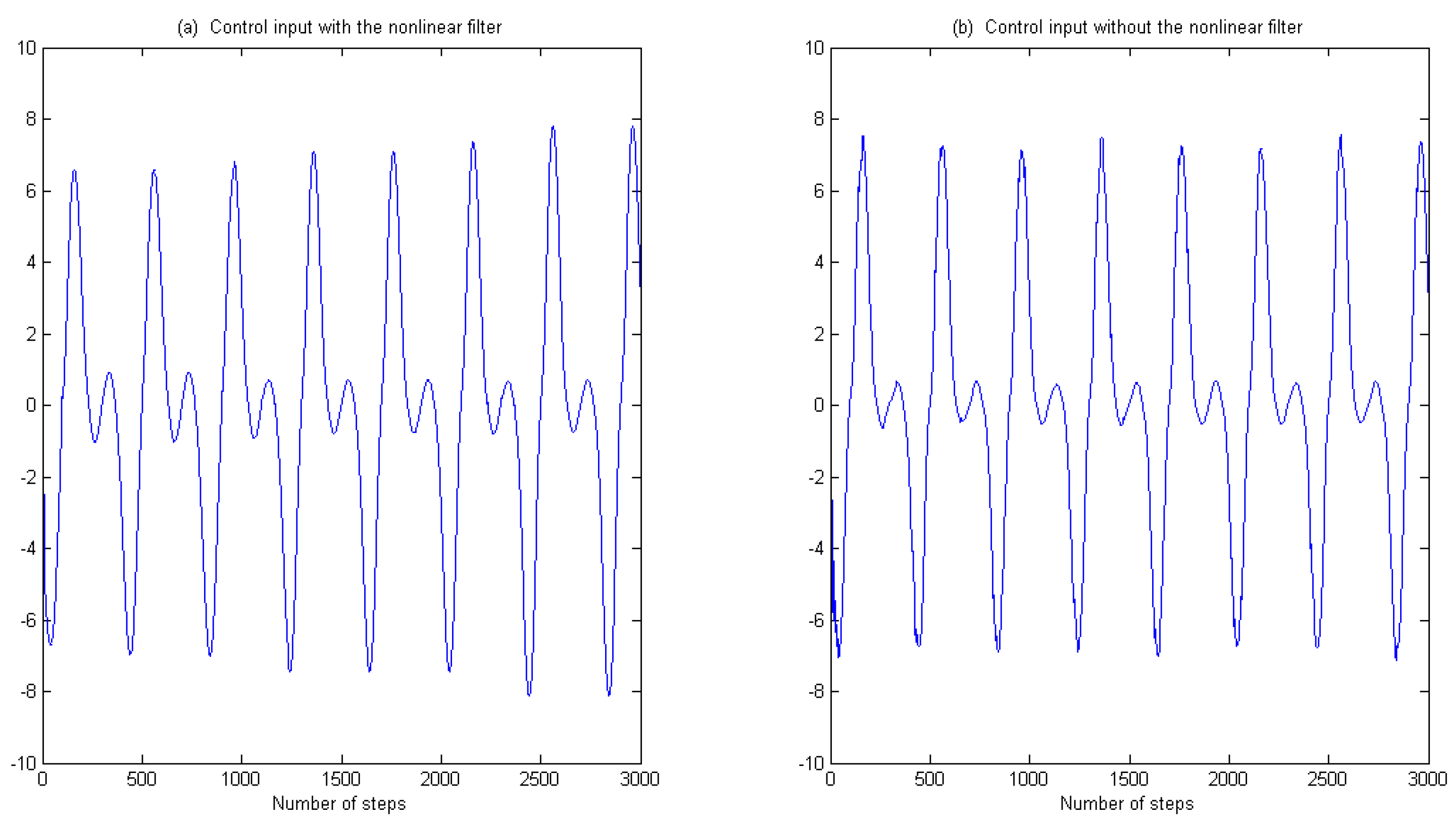
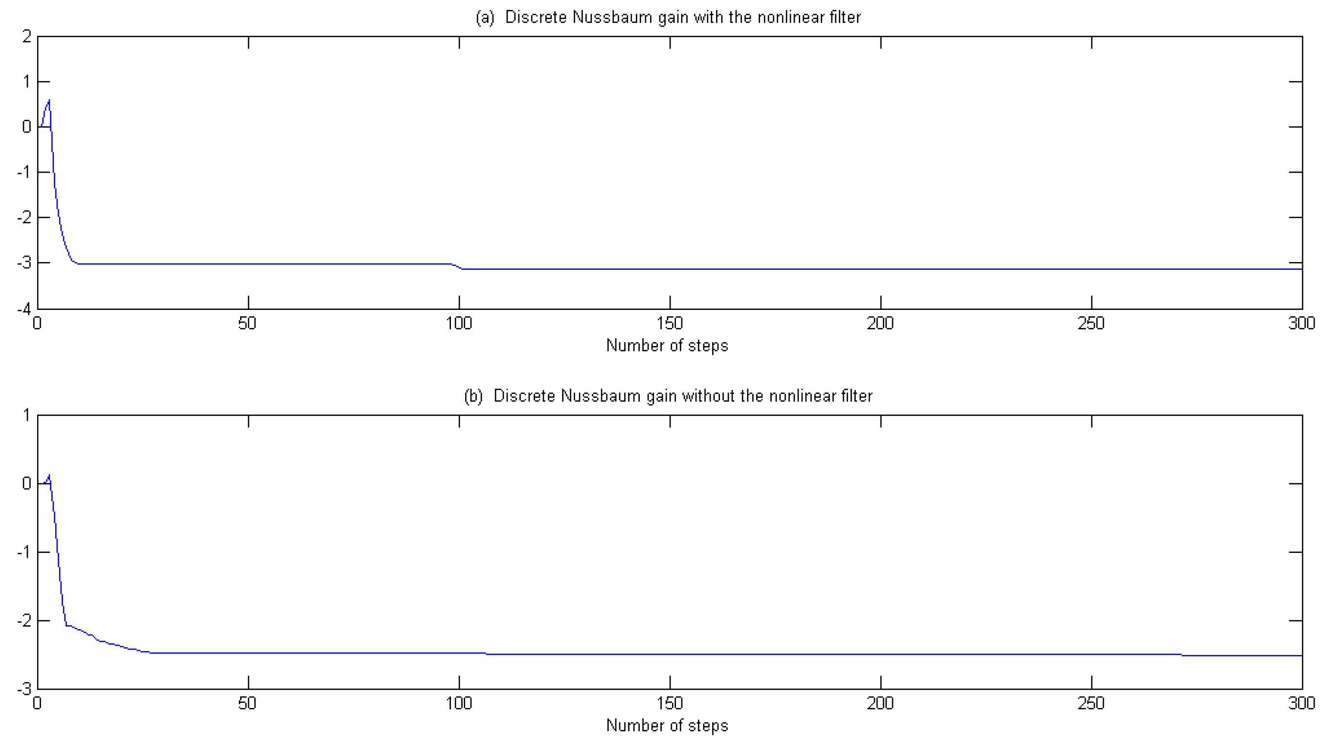
5. Illustrative Examples

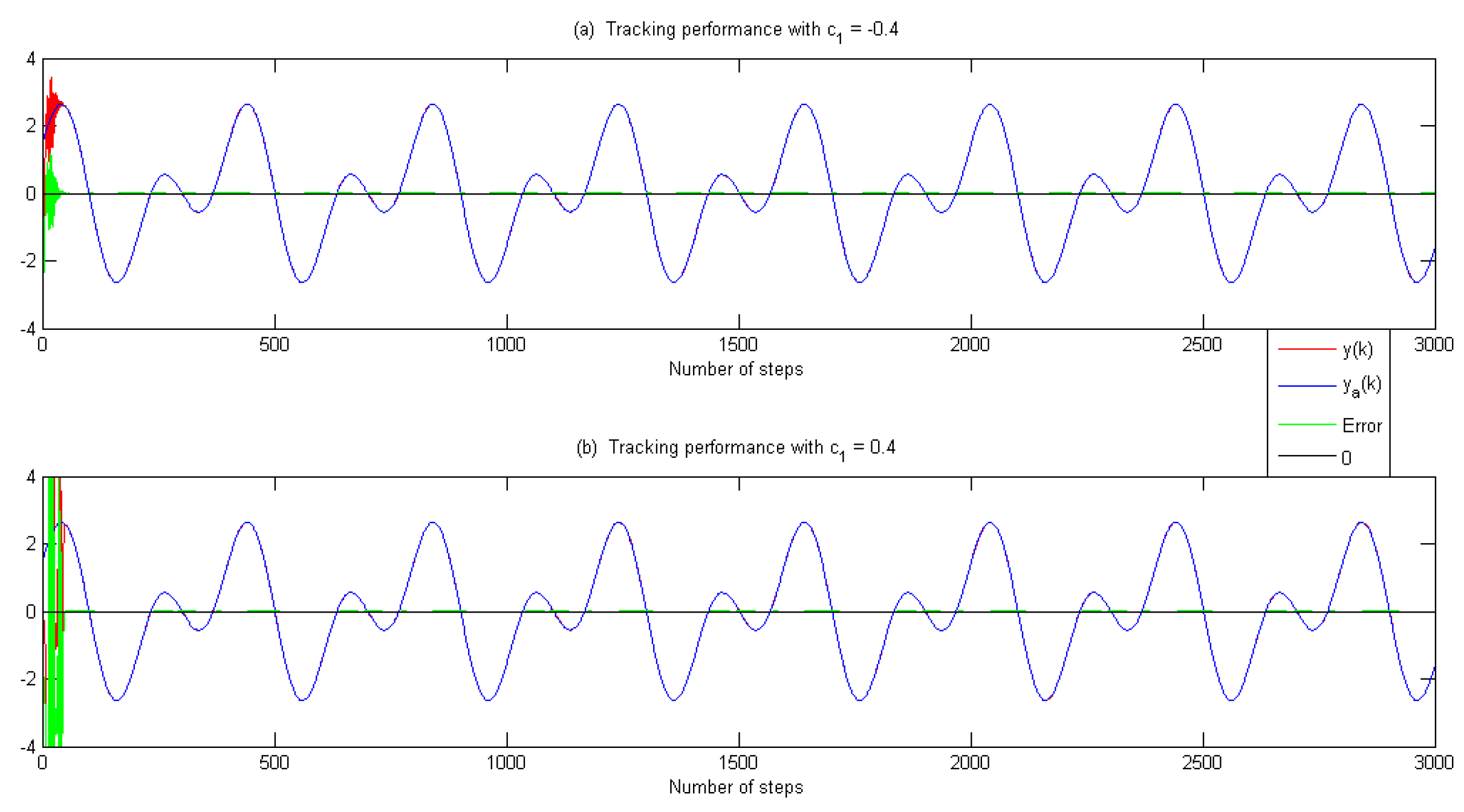
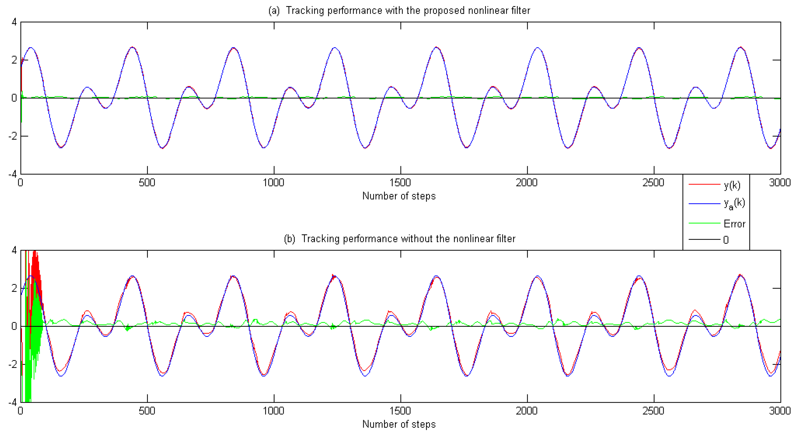
Example 1.

Consider the following no noise second-order discrete-time nonlinear system:

$$\left\{\begin{array}{l}{x}_1(k+1)=a_1{x}_1(k)\cos (x_1(k))+a_2\frac{x_1^2(k)}{1+x_1^2(k)}+g_1{x}_2(k)+c_{1}u(k),\\ x_2(k+1)=b_1\sin (x_1(k))+b_2\frac{x_1^3(k)}{2+x_1^2(k)}+g_{2}u(k),\\ \\ y(k)=x_1(k),\end{array}\right.$$

(35)

where $a_1=0.2$,  $a_2=0.1$,  $b_1=0.3$,  $b_2=-0.6$,  $g_1=1$,  $g_2=-0.2$, and  $c_1=\mp 0.4$. The initial states are  $\left[x_1(0),\hspace{0.33em}{x}_2(0)\right]=\left[1.2,\hspace{0.33em}2.0\right]$. The  $y_a(k)=1.5\sin (\frac{\pi }{5}k\mathrm{T})+1.5\cos (\frac{\pi }{10}k\mathrm{T})$, $\mathrm{T}=0.05$, is the desired reference trajectory. The extended adaptive tuning sequence is taken as $\gamma (k)=4-3·{\mathrm{e}}^{-p(k)}.$

By using the general adaptive control (8) with recursive parameter update law (15), the simulation is implemented twice to prove that the adaptability of the control system remains unaffected by variations in the feed-forward gain direction $c_1$, which is associated with the first subsystem state. Thus, the term $c_1$ is assumed to be a negative value in the first time. Then, a positive $c_1$ is assumed in the second run of the simulated system. The results are shown in Figure 3, Figure 4 and Figure 5. Figure 3 not only displays a comparison of the output and the reference, but also presents a comparison of the tacking error and benchmark 0. It is clear that, with either a negative or positive gain $c_1$, the adaptive method is effective in the no noise case. The boundedness of the control input is illustrated in Figure 4. Finally, the discrete Nussbaum gain $N(x(k))$ is shown in Figure 5. It is easy to see that the discrete Nussbaum gain searches within two directions to detect the parameter updating direction.

Example 2.

In the presence of input noise and output noise, consider a similar discrete nonlinear system:

$$\left\{\begin{array}{l}{x}_1(k+1)=a_1{x}_1(k)\cos (x_1(k))+a_2\frac{x_1^2(k)}{1+x_1^2(k)}+g_1{x}_2(k)+c_1\left(u(k)+w_u(k)\right),\\ x_2(k+1)=b_1\sin (x_1(k))+b_2\frac{x_1^3(k)}{2+x_1^2(k)}+g_2\left(u(k)+w_u(k)\right),\\ \\ y(k)=x_1(k)+w_y(k).\end{array}\right.$$

(36)

where  $a_1=0.2$, $a_2=0.1$,  $b_1=0.3$,  $b_2=-0.6$,  $g_1=1$,  $g_2=-0.2$, and $c_1=-0.4$. In Equation (36), the input noise and the output noise satisfy

$$\left\{\begin{array}{l}{w}_u(k)=0.1\cos (0.1k)\cos (x_2(k))-0.05,\\ w_y(k)=0.1\sin (0.1k)\sin (x_1(k))+0.07.\end{array}\right.$$

The initial states and the desired reference trajectory are the same as in Example 1. By using the nonlinear filtering method in (26)–(31), and by applying the adaptive control (33) with recursive parameter update law (34), we can obtain the tracking performance of the filtered output $\stackrel{⌢}{y}(k)$. It should be noted that the extended adaptive tuning sequence and the threshold value are taken as $\gamma (k)=4-3·{\mathrm{e}}^{-p(k)}$ and $\sigma =0.1$, respectively.

In addition, the results of using the nonlinear filter, compared with the results, provided by using the general adaptive method, which is described in Section 3. Comparative results are shown in Figure 6, Figure 7 and Figure 8. Figure 6 compares tracking performance. Input boundedness and discrete Nussbaum gains are illustrated in Figure 7 and Figure 8, respectively.

Example 3.

Consider the case with the positive term  $c_1=0.4$. In the presence of the same input noise and the same output noise as Example 2, the simulation model and all the other system parameters also remain the same as Example 2. The initial states and the desired reference trajectory are the same as Example 1. By using the nonlinear filter and the corresponding adaptive control scheme, the tracking performance of the filtered output  $\stackrel{⌢}{y}(k)$  can be obtained. The threshold value is set to  $\sigma =0.1.$

Similar to Example 2, the comparative results of different adaptive control schemes are presented in Figure 9, Figure 10 and Figure 11. A comparison of tracking performance is shown in Figure 9. Further, Figure 10 illustrates the results of input boundedness. A comparison of the discrete Nussbaum gain is described in Figure 11.

From Examples 2 and 3 and Figure 6, Figure 7, Figure 8, Figure 9, Figure 10 and Figure 11, we can draw the following conclusions:

• No matter if $c_1>0$ or $c_1<0$, the nonlinear filter-based adaptive control method can show tracking performance more accurately than the general adaptive control scheme;
• In order to track the reference trajectory, both the small overshoot and the short settling time are realized via the nonlinear filter-based adaptive control method;
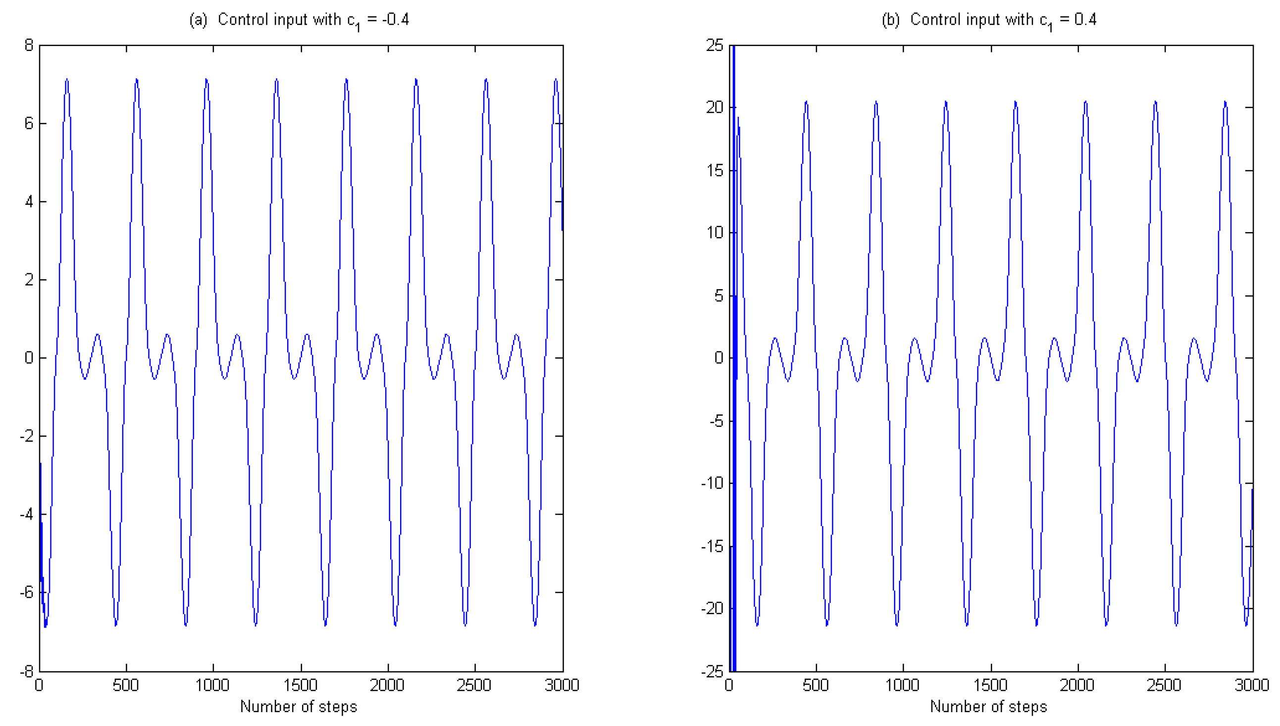
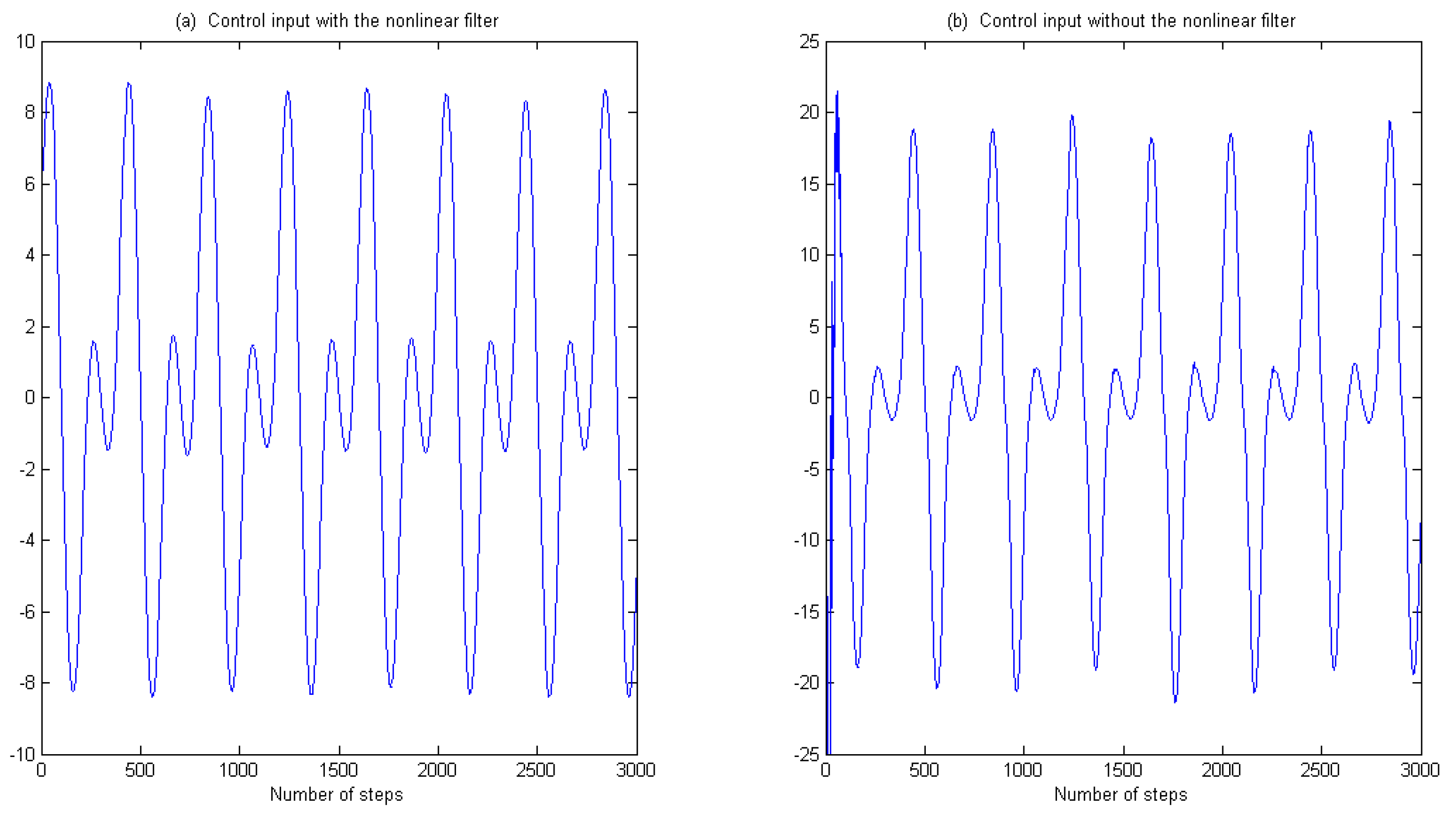
• The control inputs are bounded in all of the comparative examples;
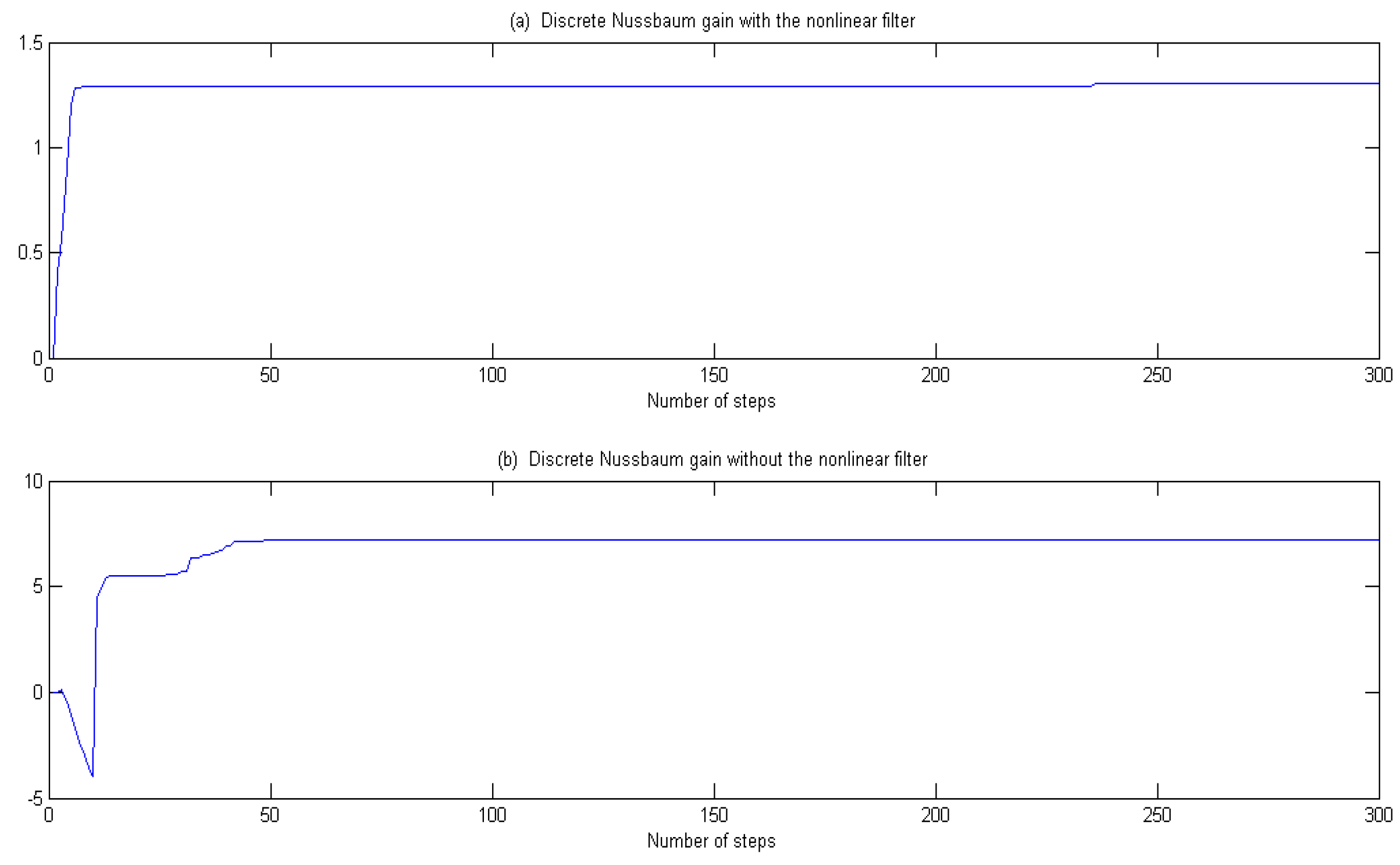
• Discrete Nussbaum gains, adopted in the proposed identification algorithm, can be designed to detect the direction of model parameters within two direction.

6. Conclusions

In this paper, a novel nonlinear filter-based adaptive control method is proposed and introduced to a subset of nonlinear discrete-time systems subject to input and output noise. The method incorporates both input feed-forward and output feedback. To address the issue of determining the direction of parameter estimation updates, the discrete Nussbaum gain is utilized, along with an extended adaptive tuning sequence to expedite the updating process. This method is also applicable to noise-free systems, and the convergence of noise-free systems is proven. In the presence of input and output noise interference, inspired by the Kalman filter equations, the time update and measurement update equations are extended to nonlinear filters, and the convergence of the algorithm is demonstrated. Compared to general adaptive control methods without filtering, this approach exhibits adaptive control rate changes alongside parameter model variations during identification. It offers better parameter trajectory tracking and timeliness. In contrast, traditional identification methods maintain a fixed control rate that does not change with the estimated parameters. The nonlinear filter-based adaptive control provides more accurate filtered output and better tracking of reference trajectories. The theoretical findings are validated through simulation results. This method can be applied in engineering practices to achieve robust adaptive control of such nonlinear systems.

References

1. Xu, Y.; Li, C.; Wang, X. Joint estimation method with multi-innovation unscented Kalman filter based on fractional-order model for state of charge and state of health estimation. Sustainability 2022, 14, 15538. [Google Scholar] [CrossRef]
2. Windmeijer, F. Two-stage least squares as minimum distance. Econom. J. 2019, 22, 1–9. [Google Scholar] [CrossRef]
3. Jia, L.; Li, X.; Chiu, M. The identification of neuro-fuzzy based MIMO Hammerstein model with separable input signals. Neurocomputing 2016, 174, 530–541. [Google Scholar] [CrossRef]
4. Xu, S.; Fan, Z. Iterative Alpha Expansion for estimating gradient-sparse signals from linear measurements. J. R. Stat. Soc. Ser. B 2021, 83, 271–292. [Google Scholar] [CrossRef]
5. Zhang, T.; Ge, S.S.; Hang, C.C. Adaptive neural network control for strict-feedback nonlinear systems using backstepping design. In Proceedings of the 1999 American Control Conference (ACC), San Diego, CA, USA, 2–4 June 1999. [Google Scholar]
6. Chen, W.; Jiao, L.; Li, J.; Li, R. Adaptive NN backstepping output-feedback control for stochastic nonlinear strict-feedback systems with time-varying delays. IEEE Trans. Syst. Man Cybern. B Cybern. 2010, 40, 939–950. [Google Scholar] [CrossRef] [PubMed]
7. Wang, D.; Huang, J. Neural network-based adaptive dynamic surface control for a class of uncertain nonlinear systems in strict-feedback form. IEEE Trans. Neural Netw. 2005, 16, 195–202. [Google Scholar] [CrossRef] [PubMed]
8. Tong, S.; Liu, C.; Li, Y. Fuzzy-adaptive decentralized output-feedback control for large-scale nonlinear systems with dynamical uncertainties. IEEE Trans. Fuzzy Syst. 2010, 18, 845–861. [Google Scholar] [CrossRef]
9. Chen, B.; Liu, X.; Tong, S. Adaptive fuzzy output tracking control of MIMO nonlinear uncertain systems. IEEE Trans. Fuzzy Syst. 2007, 15, 287–300. [Google Scholar] [CrossRef]
10. Tong, S.; Li, Y.; Shi, P. Observer-based adaptive fuzzy backstepping output feedback control of uncertain MIMO pure-feedback nonlinear systems. IEEE Trans. Fuzzy Syst. 2012, 20, 771–785. [Google Scholar] [CrossRef]
11. Chen, M.; Ge, S.S.; Voon Ee How, B. Robust adaptive neural network control for a class of uncertain MIMO nonlinear systems with input nonlinearities. IEEE Trans. Neural Netw. 2010, 21, 796–812. [Google Scholar] [CrossRef]
12. Goodwin, G.; Ramadge, P.J.; Caines, P.E. Discrete-time multivariable adaptive control. IEEE Trans. Autom. Control 1980, 25, 449–456. [Google Scholar] [CrossRef]
13. Narendra, K.S.; Lin, Y.H. Stable Discrete Adaptive Control. IEEE Trans. Autom. Control 1980, 25, 456–461. [Google Scholar] [CrossRef]
14. Yang, C.; Zhai, L.; Ge, S.S.; Chai, T.; Lee, T.H. Adaptive model reference control of a class of MIMO discrete-time systems with compensation of nonparametric uncertainty. In Proceedings of the 2008 American Control Conference (ACC), Seattle, WA, USA, 11–13 June 2008. [Google Scholar]
15. Hu, C.; Ji, Y.; Ma, C. Joint two-stage multi-innovation recursive least squares parameter and fractional-order estimation algorithm for the fractional-order input nonlinear output-error autoregressive model. Int. J. Adapt. Control Signal Process. 2023, 37, 1650–1670. [Google Scholar] [CrossRef]
16. Ding, F.; Liu, X.; Liu, G. Identification methods for Hammerstein nonlinear systems. Digit. Signal Process. 2011, 21, 215–238. [Google Scholar] [CrossRef]
17. Ding, F.; Zhu, Q. Separable synchronous multi-innovation gradient-based iterative signal modeling from on-line measurements. IEEE Trans. Instrum. Meas. 2022, 71, 6501313. [Google Scholar]
18. Bi, Y.; Ji, Y. Parameter estimation of fractional-order Hammerstein state space system based on the extended Kalman filter. Int. J. Adapt. Control Signal Process. 2023, 37, 1827–1846. [Google Scholar] [CrossRef]
19. Liu, W.; Li, M. Unbiased recursive least squares identification methods for a class of nonlinear systems with irregularly missing data. Int. J. Adapt. Control Signal Process. 2023, 37, 2247–2275. [Google Scholar] [CrossRef]
20. Chen, F.; Ding, F. Maximum likelihood based multi-innovation stochastic gradient estimation for controlled autoregressive ARMA systems using the data filtering technique. In Proceeding of the 11th World Congress on Intelligent Control and Automation, Shenyang, China, 29 June–4 July 2014; pp. 5993–5998. [Google Scholar]
21. Wang, W. Two-stage gradient-based iterative algorithms for the fractional-order nonlinear systems by using the hierarchical identification principle. Int. J. Adapt. Control Signal Process. 2022, 36, 1778–1796. [Google Scholar] [CrossRef]
22. Gu, Y.; Zhu, Q.; Nouri, H. Identification and U-control of a state-space system with time-delay. Int. J. Adapt. Control Signal Process. 2022, 36, 138–154. [Google Scholar] [CrossRef]
23. Ding, F. State filtering and parameter estimation for state space systems with scarce measurements. Signal Process. 2022, 104, 369–380. [Google Scholar] [CrossRef]
24. Ding, F. Combined state and least squares parameter estimation algorithms for dynamic systems. Appl. Math. Model. 2014, 38, 403–412. [Google Scholar] [CrossRef]
25. Wang, X.; Zhu, F.; Ding, F. The modified extended Kalman filter based recursive estimation for Wiener nonlinear systems with process noise and measurement noise. Int. J. Adapt. Control Signal Process. 2020, 34, 1321–1340. [Google Scholar] [CrossRef]
26. Xu, L.; Ding, F.; Yang, E. Auxiliary model multi-innovation stochastic gradient parameter estimation methods for nonlinear sandwich systems. Int. J. Robust Nonlinear Control 2020, 31, 148–165. [Google Scholar] [CrossRef]
27. Fan, Y.; Liu, X. Auxiliary model-based multi-innovation recursive identification algorithms for an input nonlinear controlled autoregressive moving average system with variable-gain nonlinearity. Int. J. Adapt. Control. Signal Process. 2021, 36, 521–540. [Google Scholar] [CrossRef]
28. Liu, J.; Tan, J.; Ge, X. Blind deblurring with fractional-order calculus and local minimal pixel prior. J. Vis. Commun. Image Represent. 2022, 89, 103645. [Google Scholar] [CrossRef]
29. Chen, L.; Wang, S.; Jiang, H. An adaptive fractional-order unscented Kalman filter for Li-ion batteries in the energy storage system. Indian J. Phys. 2022, 96, 3933–3939. [Google Scholar] [CrossRef]
30. Moghaddam, J.; Mojallali, H.; Teshnehlab, M. A multiple-input-single-output fractional-order Hammerstein model identification based on modified neural network. Math. Methods Appl. Sci. 2018, 41, 6252–6271. [Google Scholar] [CrossRef]
31. Zhang, J. Self-tuning control based on multi-innovation stochastic gradient parameter estimation. Syst. Control Lett. 2009, 58, 69–75. [Google Scholar] [CrossRef]
32. Ding, F.; Chen, T.; Iwai, Z. Adaptive digital control of Hammerstein nonlinear systems with limited output sampling. SIAM J. Control Optim. 2007, 45, 2257–2276. [Google Scholar] [CrossRef]
33. Ding, F. Least squares parameter estimation and multi-innovation least squares methods for linear fitting problems from noisy data. J. Comput. Appl. Math. 2023, 426, 115107. [Google Scholar] [CrossRef]
34. Ding, F.; Xu, L.; Zhang, X.; Ma, H. Hierarchical gradient- and least-squares-based iterative estimation algorithms for input-nonlinear output-error systems from measurement information by using the over-parameterization. Int. J. Robust Nonlinear Control 2023, 34, 1120–1147. [Google Scholar] [CrossRef]
35. Ding, F.; Xu, L.; Zhang, X.; Zhou, Y. Filtered auxiliary model recursive generalized extended parameter estimation methods for Box Jenkins systems by means of the filtering identification idea. Int. J. Robust Nonlinear Control 2023, 33, 5510–5535. [Google Scholar] [CrossRef]
36. Xu, L. Parameter Estimation for Nonlinear Functions Related to System Responses. Int. J. Control Autom. Syst. 2023, 21, 1780–1792. [Google Scholar] [CrossRef]
37. Xu, L. Separable newton recursive estimation method through system responses based on dynamically discrete measurements with increasing data length. Int. J. Control Autom. Syst. 2022, 20, 432–443. [Google Scholar] [CrossRef]
38. Lee, T.H.; Narendra, K.S. Stable discrete adaptive control with unknown high-frequency gain. IEEE Trans. Autom. Control 1986, 31, 477–479. [Google Scholar]
39. Chen, L.; Narendra, K.S. Nonlinear adaptive control using neural networks and multiple models. Automatica 2001, 37, 1245–1255. [Google Scholar] [CrossRef]
40. Goodwin, G.C.; Sin, K.S. Adaptive Filtering Prediction and Control; Prentice-Hall: Englewood Cliffs, NJ, USA, 1984. [Google Scholar]
41. Yang, C.; Ge, S.S.; Lee, T.H. Output feedback adaptive control of a class of nonlinear discrete-time systems with unknown control directions. Automatica 2009, 45, 270–276. [Google Scholar] [CrossRef]
42. Ge, S.S.; Yang, C.; Lee, T.H. Adaptive robust control of a class of nonlinear strict-feedback discrete-time systems with unknown control directions. Syst. Control Lett. 2008, 57, 888–895. [Google Scholar]
43. Yang, C.; Ge, S.S.; Xiang, C.; Chai, T.; Lee, T.H. Output feedback NN control for two classes of discrete-time systems with unknown control directions in a unified approach. IEEE Trans. Neural Netw. 2008, 19, 1873–1886. [Google Scholar] [CrossRef]
44. Yeh, P.C.; Kokotović, P.V. Adaptive control of a class of nonlinear discrete-time systems. Int. J. Control 1995, 62, 303–324. [Google Scholar] [CrossRef]
45. Zhang, Y.; Wen, C.; Soh, Y.C. Discrete-time robust backstepping adaptive control for nonlinear time-varying systems. IEEE Trans. Autom. Control 2000, 45, 1749–1755. [Google Scholar] [CrossRef]
46. Zhang, Y.; Wen, C.; Soh, Y.C. Robust adaptive control of uncertain discrete-time systems. Automatica 1999, 35, 321–329. [Google Scholar] [CrossRef]
47. Zhang, Y.; Wen, C.; Soh, Y.C. Robust adaptive control of nonlinear discrete-time systems by backstepping without over-parameterization. Automatica 2001, 37, 551–558. [Google Scholar] [CrossRef]
48. Ge, S.S.; Yang, C.; Dai, S.L.; Jiao, Z.; Lee, T.H. Robust adaptive control of a class of nonlinear strict-feedback discrete-time systems with exact output tracking. Automatica 2009, 45, 2537–2545. [Google Scholar] [CrossRef]
49. Yang, Y.X.; He, H.B.; Xu, G.C. Adaptively robust filtering for kinematic geodetic positioning. J. Geod. 2001, 75, 109–116. [Google Scholar] [CrossRef]
50. Rigatos, G.G. Nonlinear Kalman Filters and Particle Filters for integrated navigation of unmanned aerial vehicles. Robot. Auton. Syst. 2012, 60, 978–995. [Google Scholar] [CrossRef]
51. Gandhi, M.; Mili, L. Robust Kalman filter based on a generalized maximum-likelihood-type estimator. IEEE Trans. Signal Proces. 2010, 58, 2509–2520. [Google Scholar] [CrossRef]
52. Boutayeb, M.; Rafaralahy, H.; Darouach, M. Convergence analysis of the extended Kalman filter used as an observer for nonlinear deterministic discrete-time systems. IEEE Trans. Autom. Control 1997, 42, 581–586. [Google Scholar] [CrossRef]
Figure 1. A third-order nonlinear system with input feed-forward and output feedback.
Processes 12 00171 g001
Figure 2. Flowchart of the robust adaptive control scheme based on a novel nonlinear filter.
Processes 12 00171 g002
Figure 3. Tracking performance in Example 1.
Processes 12 00171 g003
Figure 4. The control input in Example 1.
Processes 12 00171 g004
Figure 5. Discrete Nussbaum gain N ( x ( k ) ) in Example 1.
Processes 12 00171 g005
Figure 6. Comparison of tracking performance in Example 2.
Processes 12 00171 g006
Figure 7. Comparison of control input in Example 2.
Processes 12 00171 g007
Figure 8. Comparison of discrete Nussbaum gain N ( x ( k ) ) in Example 2.
Processes 12 00171 g008
Figure 9. A comparison of tracking performance in Example 3.
Processes 12 00171 g009
Figure 10. A comparison of control input in Example 3.
Processes 12 00171 g010
Figure 11. A comparison of discrete Nussbaum gain N ( x ( k ) ) in Example 3.
Processes 12 00171 g011
Disclaimer/Publisher’s Note: The statements, opinions and data contained in all publications are solely those of the individual author(s) and contributor(s) and not of MDPI and/or the editor(s). MDPI and/or the editor(s) disclaim responsibility for any injury to people or property resulting from any ideas, methods, instructions or products referred to in the content.