Stochastic Modeling and Simulation of Filament Aggregation in Alzheimer’s Disease

Abstract

Alzheimer’s disease has been a serious problem for humankind, one without a promising cure for a long time now, and researchers around the world have been working to better understand this disease mathematically, biologically and computationally so that a better cure can be developed and finally humanity can get some relief from this disease. In this study, we try to understand the progression of Alzheimer’s disease by modeling the progression of amyloid-beta aggregation, leading to the formation of filaments using the stochastic method. In a noble approach, we treat the progression of filaments as a random chemical reaction process and apply the Monte Carlo simulation of the kinetics to simulate the progression of filaments of lengths up to 8. By modeling the progression of disease as a progression of filaments and treating this process as a stochastic process, we aim to understand the inherent randomness and complex spatial–temporal features and the convergence of filament propagation process. We also analyze different reaction events and observe the events such as primary as well as secondary elongation, aggregations and fragmentation using different propensities for different possible reactions. We also introduce the random switching of the propensity at random time, which further changes the convergence of the overall dynamics. Our findings show that the stochastic modeling can be utilized to understand the progression of amyloid-beta aggregation, which eventually leads to larger plaques and the development of Alzheimer disease in the patients. This method can be generalized for protein aggregation in any disease, which includes both the primary and secondary aggregation and fragmentation of proteins.

1. Introduction and Motivation

Alzheimer’s disease, also abbreviated as AD, is one of the most common forms of dementia, which is characterized by memory loss and cognitive decline. As of 2023, 6.7 million people are living with AD in United States [1] and over 55 million worldwide [2]. Nearly 60–80% of dementia cases comprise Alzheimer’s [2,3]. There are over 10 million new cases of dementia each year worldwide [4], which means, on average, 7 million of them are suffering from Alzheimer’s. And it will only increase each year [1] unless a satisfactory cure is invented. There are two main hypotheses from which the mathematical models have emerged. These hypotheses are used to describe the progression of AD. There are thousands of studies conducted using these hypotheses [5,6,7,8]. The first hypothesis is the amyloid hypothesis [5,6,7,9,10,11,12,13,14,15], which is a neuron-centric model, and the second is the Warbug hypothesis, which is the neuron-astrocytic model [8,15,16,17]. The neuron-centric model suggests that a mutation in the nuclear genome induces the overproduction of $\left(A\beta \right)$ and tau, which become toxic to neurons [8,16,17]. The neuron-astrocytic model contends that the progression of AD is triggered by defects in the normal energy transduction process, a condition induced by mitochondrial dysregulation [8,15,17].

According to the amyloid-beta hypothesis, Alzheimer’s is a neuro-degenerative disease, where the patient’s cognitive function progressively deteriorates, which is characterized by the progressive accumulation of amyloid beta called $\left(A\beta \right)$ peptides [15,18]. The major pathological hallmarks in the brain of AD patients are amyloid plaques [5,9,10,11,12,18], and neurofibrillary tangles (NFTs) formed by hyperphosphorylated tau protein [5]. Neurofibrillary tangles (NFT) are pathological insoluble aggregates of hyperphosphorylated tau proteins, which are microtubule-associated proteins, observed within the neurons of AD patients [12]. In healthy individuals, normal tau stabilizes the microtubules of the neuronal cytoskeleton; among their diverse functions, microtubules facilitate the transport of substances between nerve cell compartments. Aggregated tau filaments cannot be degraded by the host neurons and gradually accumulate and aggregate into insoluble filaments [11]. Tau pathology is an early feature of AD, and the appearance of tangles correlates with neuronal loss [19].

Amyloid beta is normally secreted from cells and degraded, and it is produced throughout one’s life, but in the case of AD patients, it is secreted and aggregated into insoluble plaques [18,20,21]. $A\beta$ is a proteolytic product of amyloid precursor protein (APP), and AD neuropathology is characterized by an abnormal metabolism of APP with an excessive accumulation of $A\beta$ peptides [20,22]. $A\beta$ is believed to be the main reason for initiating the pathological cascade of the disease [23]. Amyloid plaques are hard, insoluble accumulations of beta-amyloid proteins that clump together between the neurons in the brains of AD patients [5,9,10,11,12,24]. The lesions occur in brain regions involved in learning and memory, i.e, the hippocampus, the amygdala, and in the association cortices of the frontal, temporal and parietal lobes [5].

$A\beta$ deposits in senile and neuritic plaques and hyperphosphorylated tau proteins in neurofibrillary tangles (NFTs) are extracellular and intracellular expressions, respectively, of the AD neuropathological phenotype, together with selective neuronal loss in the hippocampal and neocortical regions [25]. Figure 1 shows the complex interrelation of amyloid plaques and NFT and how they cause the loss of neurons. The presence of plaques around a neuron causes them to die, possibly by triggering an immune response in the immediate area. Tangles form inside of neurons and interfere with the cellular machinery used to create and recycle proteins, which ultimately kills the cell [24].

One of the main characteristics of cells and tissues made of proteins is the self-assembly of proteins into filaments of a particular structure [14,26,27]. Cells are sustained by cytoskeletal filaments, whereas tissues are sustained by collagen fibrils. Within all eukaryotic cells, there exists a network of filaments, which is a complex mesh of protein filaments and motor proteins that aid in cell movement and stabilize the cell [28]. And cytoskeletal filaments are equally important in the correct formation of the nervous system and their various functions [27,28]. Given the importance of the cytoskeleton for neurons, its involvement in neurological disorders (taupathies), including AD, is not surprising, and it can be in the form of their mutation and changes in their dynamics and the stability of the cytoskeletal proteins [27].

All of this self-assembly of the proteins, be it functional or dysfunctional, involves the assembly of elementary units to the ends of the growing structure [9,13,14]. Hence, on that note, we are interested in studying the early aggregation of monomers forming the structure, like oligomers and filaments. These filaments are the most toxic structure [13] and need attention for both understanding the disease and deriving the potential cure. Studies suggest that the aggregation of a primary structure, such as monomers, into the intermediate species, such as oligomers and unbreakable filaments, are correlated with cellular toxicity [13], and such is the case of most amyloid-based diseases, including AD. In AD, the aggregation of soluble APP, into non-soluble amyloid fibrils is the major cause of cognitive loss, including NFT [5,9,10,11,12].

The law of mass action serves as the foundation for robust kinetic models that effectively define the chemical kinetics of intricate reaction networks controlling the growth of filamentous protein structures. These models also provide valuable insights into the complex processes underlying protein aggregation [9]. In that respect, [9,14] established master equations to treat the aggregation of the amyloid precursor protein towards the formation of fibrils. They established the criterion for primary nucleation, elongation and other secondary events, such as secondary nucleation, fragmentation and monomer-dependent elongation [9,14]. Ref. [13] established another master equation to capture the stochastic effects in early amyloid aggregation to describe the aggregation of monomers into oligomers. They used log-normal closure moment method rather than direct simulation. They also used the Gillespie algorithm to simulate the process of protein aggregation and compared it with the result from their master equation. Ref. [6] introduced the method of second stochasticization by introducing random noises into already statistically averaged equations obtained from moment closure methods. They coupled their study with the stochastic simulation using the Gillespie algorithm. Ref. [15] used a stochastic mathematical model to understand the various phases and transitions of AD.

Due to the complexity and the number of aspects involved in the protein aggregation, although the deterministic mathematical model has given some very good frameworks, they do not capture the inherent stochastic nature present in the bio-chemical reactions. From a physical point of view, the stochastic formulation of chemical kinetics is superior to the deterministic formulation: the stochastic approach is always valid whenever the deterministic approach is valid, and is sometimes valid when the deterministic approach is not [29]. Hence, to unravel the complex dynamics preset in the amyloid-beta aggregation, we make use of the stochastic computational simulation to understand the dynamics of amyloid growth and the aggregation of monomers towards forming filaments. We study the formation of filaments from, at most, eight monomers. We treat all possible combinations of monomers forming the filaments of lengths up until eight. Our comprehensive simulation of reaction kinetics is the main contribution of our work, which sheds light on the aggregation and formation of no-soluble toxic filaments from soluble protein units. We experiment with the primary nucleation, followed by aggregation/elongation and fragmentation, which occur with different propensities. We also simulate the dynamics on different sets of propensities, using different propensities for different reaction events, which are not so evident in the studies that we reviewed. With that, we are also able to see how the individual filament of length i evolved with time, and we also evaluate the dynamics by introducing different random propensities at different times. Our experiments show that the evolution of amyloid-beta aggregation can be modeled computationally by using stochastic modeling techniques of chemical reactions. We evaluate the convergence by plotting the phase diagram of the evolution of filaments of different lengths, and by also plotting the zeroth moment and first moment. We also find that the convergence is highly correlated with the propensities used for the reaction events, and some events dominate the overall reactions events that occur during the simulation. And there is a clear difference in convergence when we use fixed constants for each reaction and different constants for different reactions. We also evaluate that the initial conditions (the initial population of pre-existing filaments) affect the final convergence.

Although some 90,000+ research studies have been published since 1990 on AD [25], it still remains an enigma largely due to the nature of the disease and its complexity [25,30]. Although the amyloid-beta hypothesis has been studied widely and believed to show the development of disease, it is still very hard to trace the root of the disease, or how, why and when it develops [19,25,30]. And there is more and more speculation that $A\beta$ plaques are the result of AD, and not the other way around [30]. But it is clear from all these studies that $A\beta$ and $NFT$ are well-known markers of AD, and hence are worth studying further. On that note, we think that there is a space for contribution to be made in the stochastic nature of the $A\beta$ aggregation, and how they propagate and form the dysfunctional insoluble filaments. Hence, the main objective of this work is to utilize the mathematical and computational framework to unravel the stochastic nature of the elongation, propagation and possible fragmentation of $A\beta$ peptides. We treat this process as a chemical reaction process and use the chemical kinetics of the intricate reaction, which is responsible for forming the filamentous protein structure. Our main contribution lies in conducting detailed simulations and reaction kinetics analyses to understand the stochastic nature of amyloid-beta aggregation, which includes experimenting with various reaction propensities and their random switching over time, thus providing a comprehensive model of amyloid-beta aggregation as a stochastic chemical reaction process, an approach not extensively explored in previous studies.

The paper is organized as follows: This first section introduces the work, the motivation behind this study, and the objectives. Section 3 introduces the mathematical theory behind the chemical reaction and how the stochastic modeling can be performed. Section 4 shows the experiments that we conducted comprehensively. In the last three sections, we discuss the results, limitations and conclusions.

2. Chemical Reaction Network: Mathematical Theory

The mathematical theory behind modeling chemical reactions with stochastic processes involves the use of the chemical master equation, which describes the time evolution of the probability distribution of the state of a chemical system. The chemical master equation can be derived from the principle of detailed balance, which states that the rate of each reaction is balanced by the reverse reaction, ensuring that the system is in a state of equilibrium.

2.1. Chemical Reaction Networks

Chemical reaction networks (CRNs) involve the interactions of molecular units within a multi-variable dynamical system. In deterministic modeling, CRNs are represented using differential equations derived from the fundamental law of mass action. The resulting system of differential equations is commonly nonlinear and often lacks an exact solution. The deterministic theory of CRNs was developed in the 1970s by Fritz Horn, Roy Jackson, and Martin Feinberg [31]. A chemical reaction network is described by the triple $\left\{S,C,R\right\}$, where S is the species, C is the complexes which are described by a non-negative linear combinations of the species that describe how the species can interact, and R represents the reactions.

2.2. Deterministic Model of Chemical Reaction Networks

A chemical reaction network characterizes the reactions of chemical species. In this regard, consider m different species $X_i$, $i=1,2,\dots ,m$, that participate in n reactions as follows [31]:

$$\sum _{j=1}^m{a}_{ij}{X}_j\stackrel{k_i}{\to }\sum _{j=1}^m{b}_{ij}{X}_j, 1\le i\le m$$

(1)

$a_{ij}$s and $b_{ij}$s are the stoichiometric coefficients, and they are non-negative integers. The reaction rates, following the law of mass action, are given by

$$r_i=k_i\prod _{j=1}^m{X}_i^{a_{ij}}$$

(2)

By defining the stoichiometric matrix S as

$$S=\left(s_{ij}\right)=(b_{ij}-a_{ij})$$

the differential equations are written as

$$\frac{dX}{dt}=Sr$$

2.3. Stochastic Models of the Chemical Reaction Network

The mathematical theory behind modeling chemical reactions with stochastic processes involves the use of the chemical master equation, which describes the time evolution of the probability distribution of the state of a chemical system. The chemical master equation can be derived from the principle of detailed balance, which states that the rate of each reaction is balanced by the reverse reaction, ensuring that the system is in a state of equilibrium [32,33].

$$\frac{dP}{dt}=Sr$$

where P is a vector of probabilities that represents the probability distribution of the state of the system, t is time, S is the stoichiometry matrix that describes the changes in the number of molecules of each species as a result of each reaction, and r is the vector of reaction rate functions that depend on the concentrations of the reactants.

Denoting by $P\left(X\right(t),t)$ the probability for the state $X\left(t\right)=(X_1\left(t\right),X_2\left(t\right),\dots ,X_n\left(t\right))$ at time t,

$$\frac{dP\left(X\right(t),t)}{dt}=\sum _{i=1}^{m}P(X-S_i,t)a_i(X-S_i)-\sum _{i=1}^{m}P(X,t)a_i\left(X\right)$$

$S_i$ is the ith row of the stoichiometric matrix S, and $a_i\left(X\right)$ is the propensity function for the ith reaction determined by the law of mass action [32,33].

3. Modeling Assumptions

The primary assumption underlying the model is that the aggregation of $A\beta$ proteins is the leading hypothesis for Alzheimer’s disease.

Cohen et al. [9,14,34] built upon Oosawa’s theory, which was originally developed to derive analytical results for filamentous growth in primary pathways, and expanded it to include possible secondary pathways [35]. Figure 2 illustrates the microscopic processes involved, namely primary nucleation, elongation, dissociation, fragmentation, and monomer-dependent secondary nucleation as described in the master equation.

$$\stackrel{\mathrm{Primary\; Nucleation}}{\overbrace{M_1+M_1⟶M_2}}\underset{\mathrm{Elongation}}{\underbrace{\stackrel{}{⟶}{M}_3}}\stackrel{\mathrm{Elongation}}{\overbrace{\stackrel{}{⟶}{M}_4\stackrel{k_{+}}{⟶}\dots \stackrel{k_{+}}{⟶}{M}_n}}\underset{\mathrm{aggregation}/\mathrm{fragmentation}}{\underbrace{\stackrel{}{⟶}{M}_{n+1}\stackrel{}{⟶}\dots ⟶M_m+M_j\stackrel{}{⟷}{M}_{m+j}}}$$

(3)

Table 1. Multi-step aggregation process of $A\beta$.

	Chemical Reactions	Reaction Rate	Explanation
$\left(1\right)$	$M_1+M_1⟶M_2$	$k_n$	Primary Nucleation
$\left(2\right)$	$M_i+M_1⟶M_{i+1}$	$k_{+}$	Elongation, $i\ge 2$
(2)	$M_i+M_1⟵M_{i+1}$	$k_{\mathrm{off}}$	Dissociation, $i\ge 2$
$\left(3\right)$	$M_i+M_j⟶M_{i+j}$	$k_{+}$	aggregation, $2\le i<\infty$
$\left(4\right)$	$M_i+M_j⟵M_{i+j}$	$k_2$	Fragmentation, $2\le i<\infty ,2\le j\le i$

shows the aggregation process and different types of reactions that can happen, it is further more illustrated in the Figure 2.

3.1. The Structural Organization of Amyloid-Beta Peptides and Amyloid Precursor Protein (APP)

Amyloid beta peptide is a 36–43 amino acid peptide and derives from precursor protein, amyloid-beta precursor protein (APP) enzymatic proteolysis, a physiologically produced protein that plays important roles in brain homeostasis [36,37]. In $A\beta$, peptides are generated with a predominance of the 40 amino acid from $\left(A\beta 40\right)$ followed by $42\left(A\beta 42\right)$. $A\beta 42$ is more prone to aggregation than $A\beta 40$. Immune histochemical analysis indicates that $A\beta 42$ is initially deposited and found at a higher concentration in the amyloid plaques observed in AD patients [36]. It is believed that the over-expression of APP results in an increase in cerebral $A\beta$ peptides and consequently in their deposition.

Some cases of early onset familial Alzheimer’s disease are linked to mutations in three genes—amyloid precursor protein (APP) on chromosome 21, presenilin 1 (PSEN1) on chromosome 14, and presenilin 2 (PSEN2) on chromosome 1, with mutations in PSEN1 being the most frequent cause of autosomal dominant Alzheimer’s disease [37]. For the more detailed treatment of the structure and organization of the $A\beta$, we refer the readers to [36,37].

3.2. Master Equation in Deterministic Form

Following [9,14,34], Equation (4) represents the master equation, which is derived based on the kinetics of these microscopic processes and their impact on the concentration changes of chains of length j over time, represented by $f(t;j)$. Equation (5) depicts the temporal variation of the free monomer concentration, denoted as $m\left(t\right)$:

$$\begin{array}{cc}& \frac{\partial f(t,i)}{\partial t}=2m\left(t\right)k_{+}f(t,j-1)-2m\left(t\right)k_{+}f(t,j)+2m\left(t\right)k_{off}f(t,j+1)-2m\left(t\right)k_{off}f(t,j)\hfill \\ & -k_{-}(j-1)f(t,j)+2k_{-}\sum _{i=j+1}^{\infty }f(t,i)+k_{2}m{\left(t\right)}^{n_2}\sum _{i=j+1}^{\infty }if(t,i){\delta }_{j,n_2}+k_{n}m{\left(t\right)}^{n_c}{\delta }_{j,n_c}\hfill \end{array}$$

(4)

$$\frac{dm\left(t\right)}{dt}=-\frac{d}{dt}[\sum _{j=n_c}^{\infty }jf(t,j)]$$

(5)

Defining the first and second moments as

$$P\left(t\right)=\sum _i^{\infty }f(t,i),M\left(t\right)=\sum _i^{\infty }if(t,i)$$

the differential equations that govern these moments are as follows [9,14]:

$$\frac{dP\left(t\right)}{dt}=k_{-}[M\left(t\right)-(2n_c-1)P\left(t\right)]+k_{2}m{\left(t\right)}^{n_2}M\left(t\right)+k_{n}m{\left(t\right)}^{n_c}$$

(6)

$$\frac{dM\left(t\right)}{dt}=2[M\left(t\right)k_{+}-k_{\mathrm{off}}-k_{-}\frac{n_c(n_c-1)}{2}]P\left(t\right)+k_{2}m{\left(t\right)}^{n_2}M\left(t\right)+n_c{k}_{n}m{\left(t\right)}^{n_c}$$

(7)

Following [9,14], in these equations, $n_c$ is the number of proteins that participate in the nucleation. The average length of the filaments is given by

$$\mu =\frac{M\left(t\right)}{P\left(t\right)}$$

3.3. Stochastic Modeling of the $A\beta$ Aggregations

The complete kinetics are provided in Tables S1 and S2 of the Supplementary Material. In our analysis of filaments up to length eight, we denote free proteins as $M_1$, while filaments with a length of eight are represented as $M_8$. Specifically, $x_1,x_2,x_3,x_4,x_5,x_6,x_7$, and $x_8$ correspond to $M_1$ to $M_8$. The chemical master equation for the model, describing the probability evolution of the system, is formulated as outlined in [13]. Below are two sample equations for the reactions $M_1+M_1\to M_2$ and $M_1+M_2\to M_3$. Similar expressions for other reactions follow the same structure, though we refrain from detailing them here for brevity:

$$\begin{array}{cc}\hfill \frac{dP(x_1,x_2,x_3,x_4,x_5,x_6,x_7,x_8,t)}{dt}=& k_n{(x_1+2)}^{2}P(x_1+2,x_2-1,x_3,x_4,x_5,x_6,x_7,x_8,t)+\hfill \\ \hfill & k_{+}(x_2+1)(x_1+1)P(x_1,x_2+1,x_3+1,x_4-1,x_5,x_6,x_7,x_8,t)+\hfill \\ \hfill \dots \end{array}$$

(8)

Given the substantial number of constants involved—54 in total—during the modeling of both the aggregation and fragmentation, our analysis primarily centers on stochastic simulations. It is worth noting that we refrain from explicitly delving into the numerical solutions of the master equation, keeping our focus squarely on the stochastic simulation.

4. Computational Simulation Results

We use the Gillespie algorithm [29], which is a seminal method for simulating the stochastic processes, and we use it to simulate the aggregation and fragmentation processes of amyloid beta. We use Monte Carlo simulation on top of the Gillespie algorithm and average out the results to reduce any anomalies that may be present in a single simulation. The general framework of the Gillespie algorithm lies in randomly picking up the next reaction time, and the next reaction event that can occur from the set of possible events. The pseudo-code for the Gillespie algorithm that we used is given in Algorithm S2 of Supplementary Material. We wrap the Gillespie function with Monte Carlo simulation and derive the average simulation results over the number of simulations. The pseudo-code for the Monte Carlo simulation is provided in the additional materials. We utilize Python to simulate the reaction processes and conduct Monte Carlo simulations. The initial experiments were performed using the Jupyter Notebook on a standard notebook/desktop, with 16 GB of memory.

Different initial conditions are used for different simulations; similarly, we experimented with different reaction rates, e.g., different aggregation rates and fragmentation rates. Firstly, we only simulated the aggregation process, and later added the secondary events such as fragmentation. The monomers are labeled as $M_1$, and when they aggregate they can take the form of filaments of length i, such as $M_i$. $M_1$, the population of free proteins, can be interpreted as amyloid precursor protein (APP), the primary nucleation which produces the oligomers, then the rest of the population can be interpreted as the aggregation of $A\beta 42$ into toxic filaments.

4.1. Modeling the Aggregation Events

To model the monomer aggregation, we first define the kinetics of aggregation, listing all possible reactions that can occur and defining their aggregation rates/constants. The table of the kinetics of amyloid-beta aggregation in the appendix shows the possible reactions that we model in this study. $M_i$ represents the filament of length i, whereas the reaction rate $k_i$ represent the reaction rate for that particular reaction. For example, $k_1$ represents the aggregation rate of $M_1$ and $M_2$, blending together to form $M_3$. In the table of reaction kinetics, there are a total of 27 different types of aggregation reactions, producing filaments of different length i.

We use the stoichiometry matrix given in the Supplementary Material Section S2.3.1, Equation (S1) derived for a total of 27 possible aggregation events for the filaments of length up until eight. The stoichiometry matrix is derived using the reaction kinetics given in Table S2.1 of Supplementary Material. In this matrix, each column represents $M_1,M_2,\dots ,M_8$, while each row describes the actual reactions. For example, two $M_1$ make $M_2$; hence, in the first row of the matrix, $M_1$ has a corresponding value $-2$, and $M_2$ has a value 1. This is essentially saying that from the total population of $M_1$, two $M_1$ were lost to create one new $M_2$. For the reaction rates, we start the rate from a certain constant, for example, $0.00001$, which is used for the result presented in Figure 3. $k_0$ starts from this initial value $0.00001$; $k_1$ is the exact half of $k_0$, $k_2$ is the exact half of $k_1$ and so on, and thus the last reaction constant $k_{26}$ is half of $k_{25}$. The rationale behind choosing such a reaction rate is that, the greater the length of the filaments, the lower the likelihood of blending with others, and similarly, the propensity of, let us say, $M_1+M_1=M_2$ is much higher than $M_2+M_2=M_4$, and the propensity of forming the filament of length eight ($M_8$) from the aggregation event $M_1+M_1+M_2+M_4=M_8$ is the least likely. These complex reactions are assumed to be less likely than two monomers joining together.

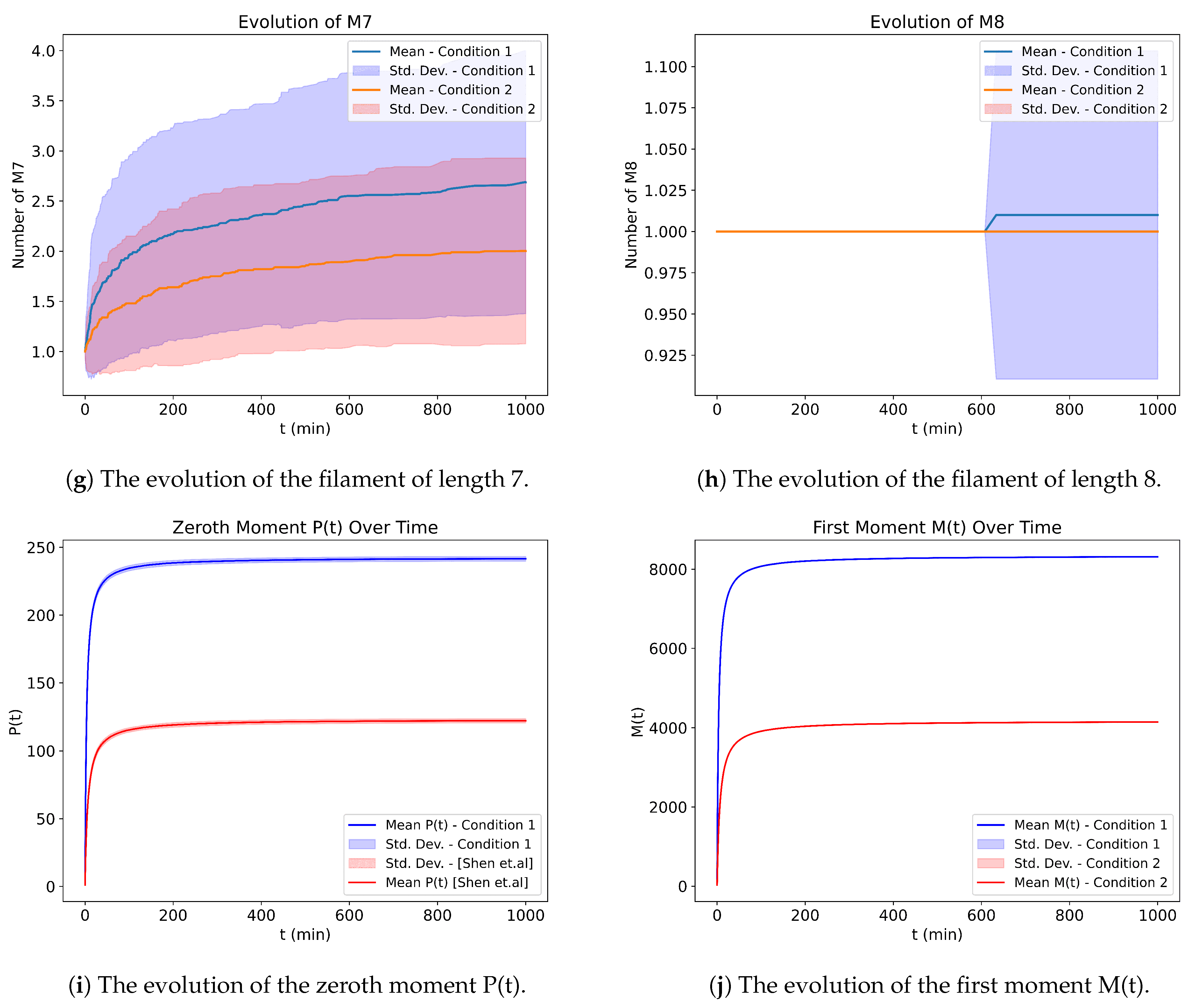
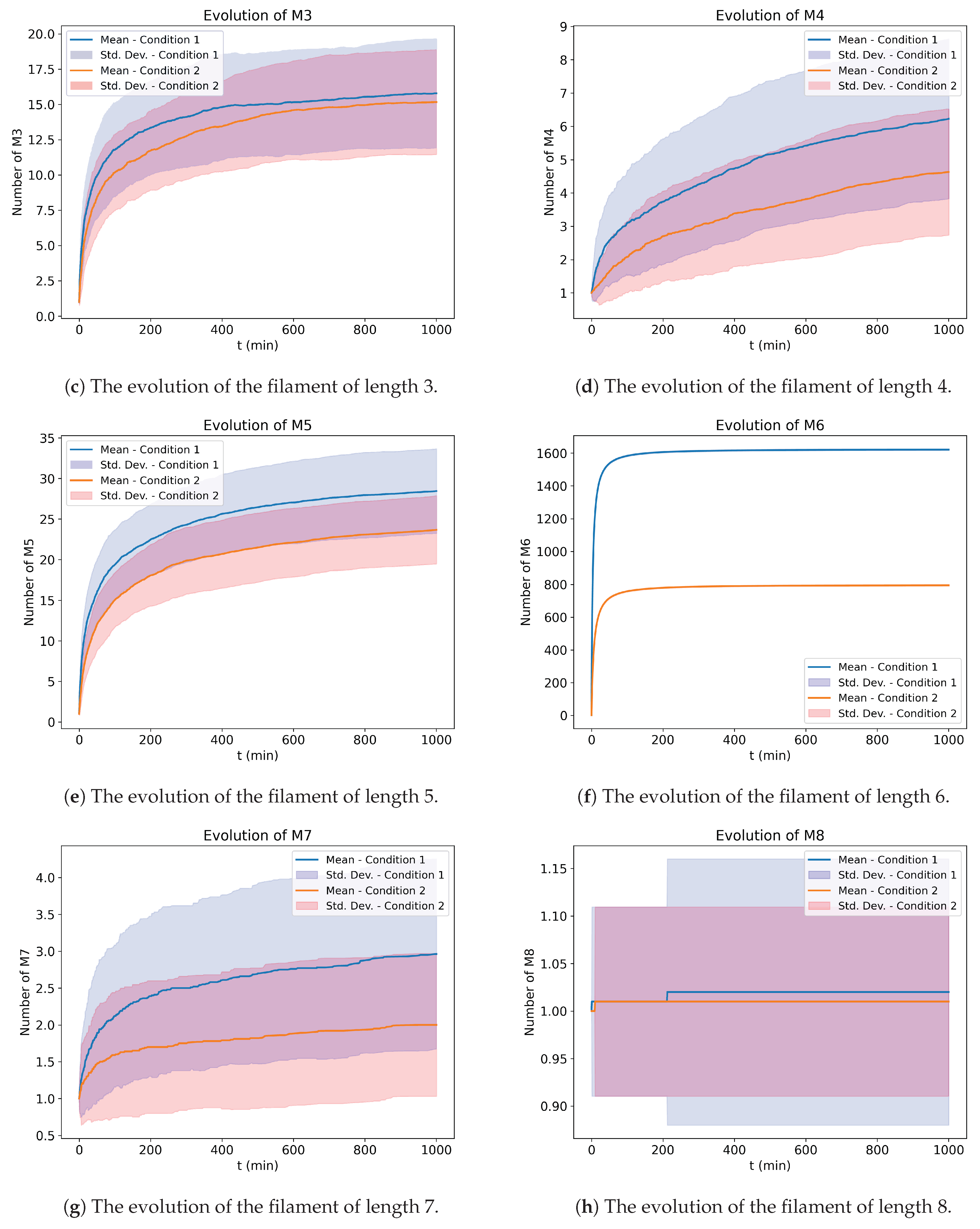
Figure 3 shows the time evolution of monomers and filaments of lengths up to eight, as we can see that there is smooth evolution of filaments of a length of six. We run 100 Monte Carlo simulations, and the average and standard deviation among the multiple simulations are shown in the shaded area. The simulation uses the matrix representation of the reaction as given in the extra materials. The essential difference in Figure 3 and Figure 4 and is the initial population of different lengths of the filaments. Our experiments for fixed constant rates with different initial conditions are in the extra material’s section, called “Aggregation of Filaments with Fixed Constant Rates”. It shows how keeping the constants fixed but changing just the initial conditions leads to different convergence.

4.2. Modeling the Aggregation and Fragmentation Events

In this section, we show the experiments conducted in different initial conditions and reaction rates, with both aggregation as well as secondary events, such as fragmentation. In Section 4.1, we only considered the aggregation events; here, we add the fragmentation events and form a different kinetics and stoichiometry matrix. The kinetics and stoichiometry matrix are provided in the Supplementary Material’s Table S2.2 the Equation (S2.3.2), respectively.

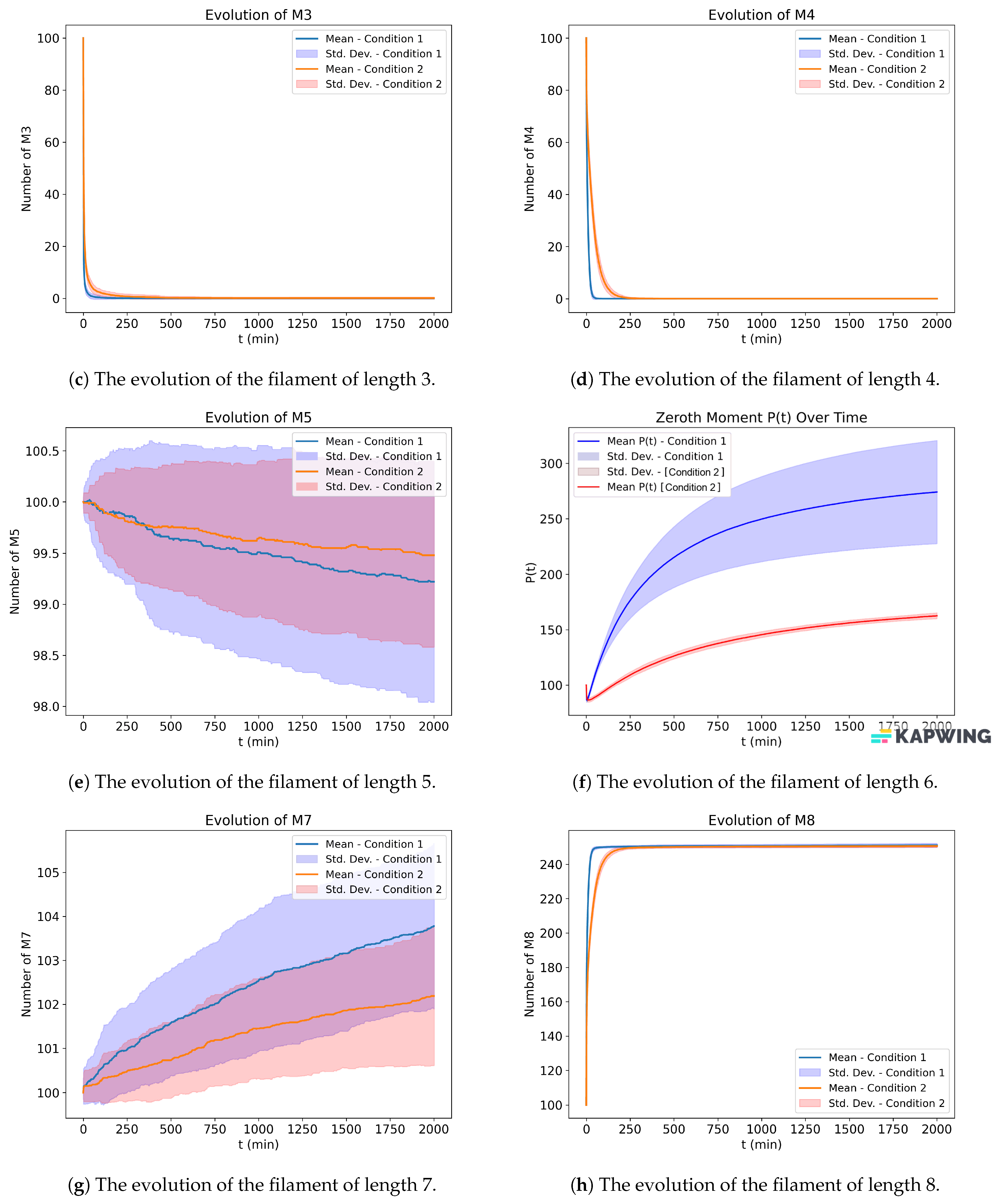
In Figure 5, we take the initial population of $M_2,\dots ,M_8$ to be 100, and in Figure 6, we keep it to be 1. We can notice the difference in convergence when we use the same reaction probabilities for the events while taking a different initial population.

Figure 7 shows how this changes when we keep the reaction rates constant (one for elongation, second for all aggregation events and third constant for fragmentation events). We denote the reduction in the overall population of filaments of length $2,\dots ,8$. Also, they are converging slower than in Figure 5, where we used different propensities for different events.

In Figure 5, different aggregation and fragmentation rates are used. The starting reaction rate for aggregation starts from $k_0=0.00001$, and the subsequent aggregation event, as listed in Table S2 (aggregation and fragmentation kinetics) in the extra material, will be exactly half of the previous one and so on. And similarly for the fragmentation, the reaction rate starts from $k_1=0.00001/2$, and each subsequent fragmentation reaction rate such as $k_3=0.00001/4$ and so on.

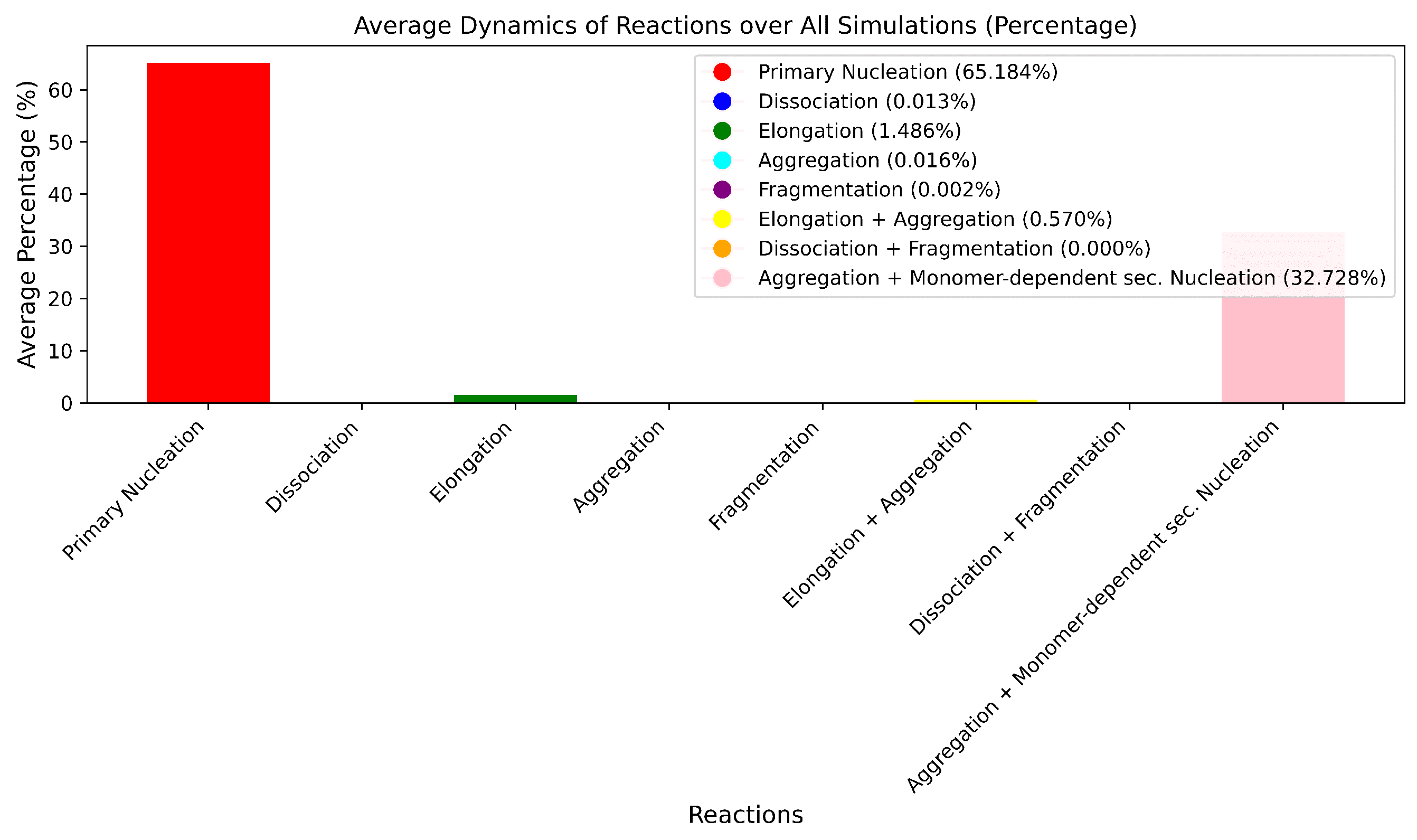
From Figure 8, it is clear that certain reaction events dominate the overall dynamics of the process. This observation is critical in understanding the inherent behavior of the system under study. Subsequently, in Figure 9, we introduce a modification to the Gillespie algorithm by incorporating random selection of reaction rates. This adaptation involves randomly choosing a reaction rate from the original set and applying it to a reaction event. We implement this change for $10\%$ of the time, allowing for the possibility of any reaction propensity to be randomly selected. When we reduce this randomness to only $1\%$ of the time, the results increasingly resemble those obtained without introducing randomness. Further reduction of the randomness leads to results that closely align with those from the original algorithm, demonstrating more uniform convergence. The impact of using random switching of reaction probabilities is evident in the results; specifically, introducing random propensities tends to decrease the converged population, thereby reducing the filament formation. This effect becomes even more apparent when we examine the evolution of individual populations.

Continuing this analysis, Figure 10 shows that the introduction of random switching of probabilities does not significantly alter the dominance of certain reaction events in the overall dynamics. This observation indicates that, despite the random elements introduced in the reaction propensities, the core characteristics of the process are largely maintained.

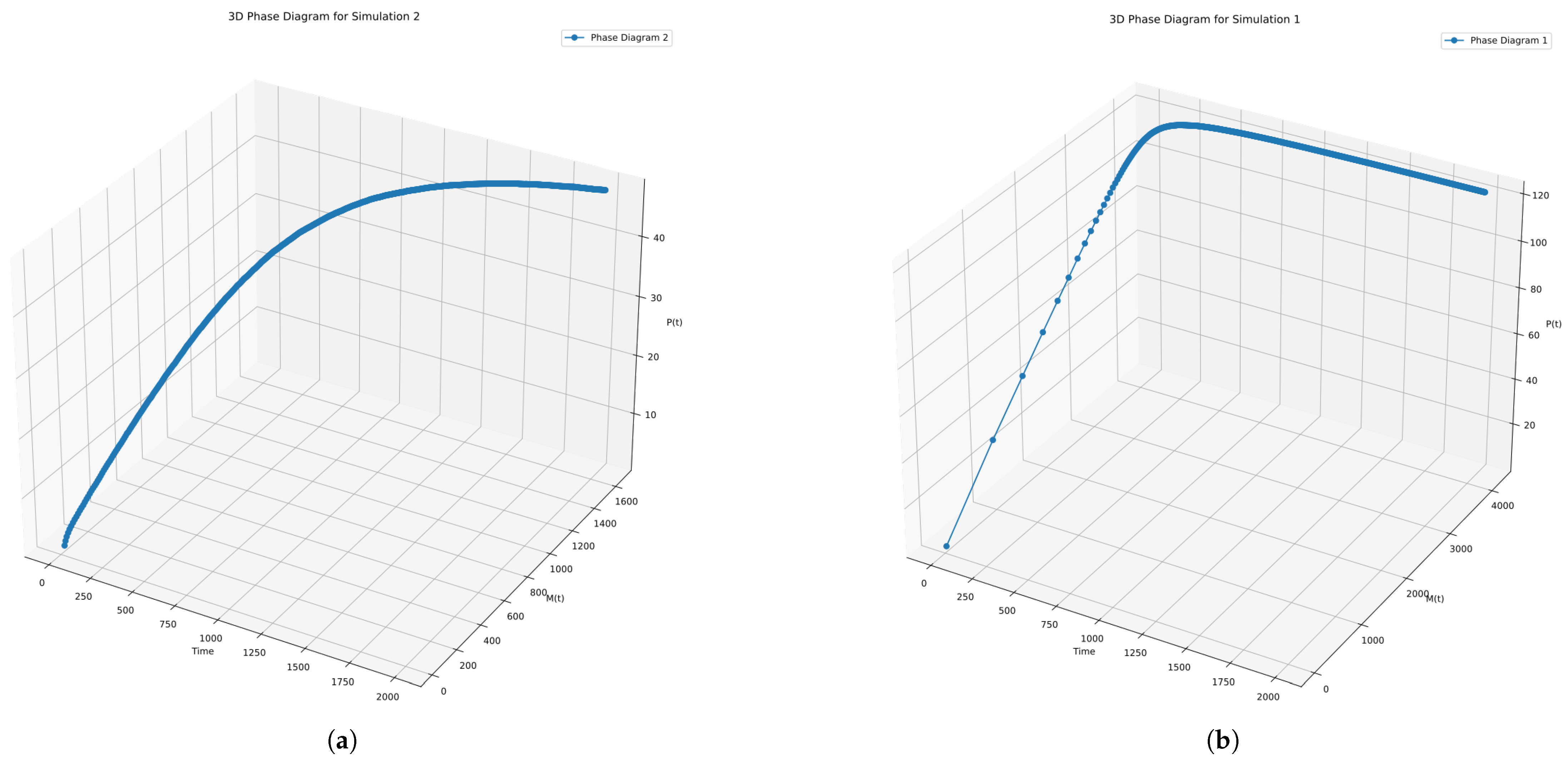
In Figure 11, we plot the phase diagram, X-axis showing the time (t), Y-axis showing the first moment M(t) and Z-axis showing the zeroth moment (P(t)). It is evident that, without the random switching of the probabilities, the dynamics tend to aggregate more filaments of different lengths than in the case of using the random switching of probabilities.

4.3. Comparison with Other Studies

In this section, we compare our results with that of [6,13]. Both of these methods implement the moment-closure method for the stochastic modeling of the aggregation of proteins in amyloid disease. First we try to model the work of [13] using their own stoichiometry but with different probabilities for the reaction events than were originally used in their work.

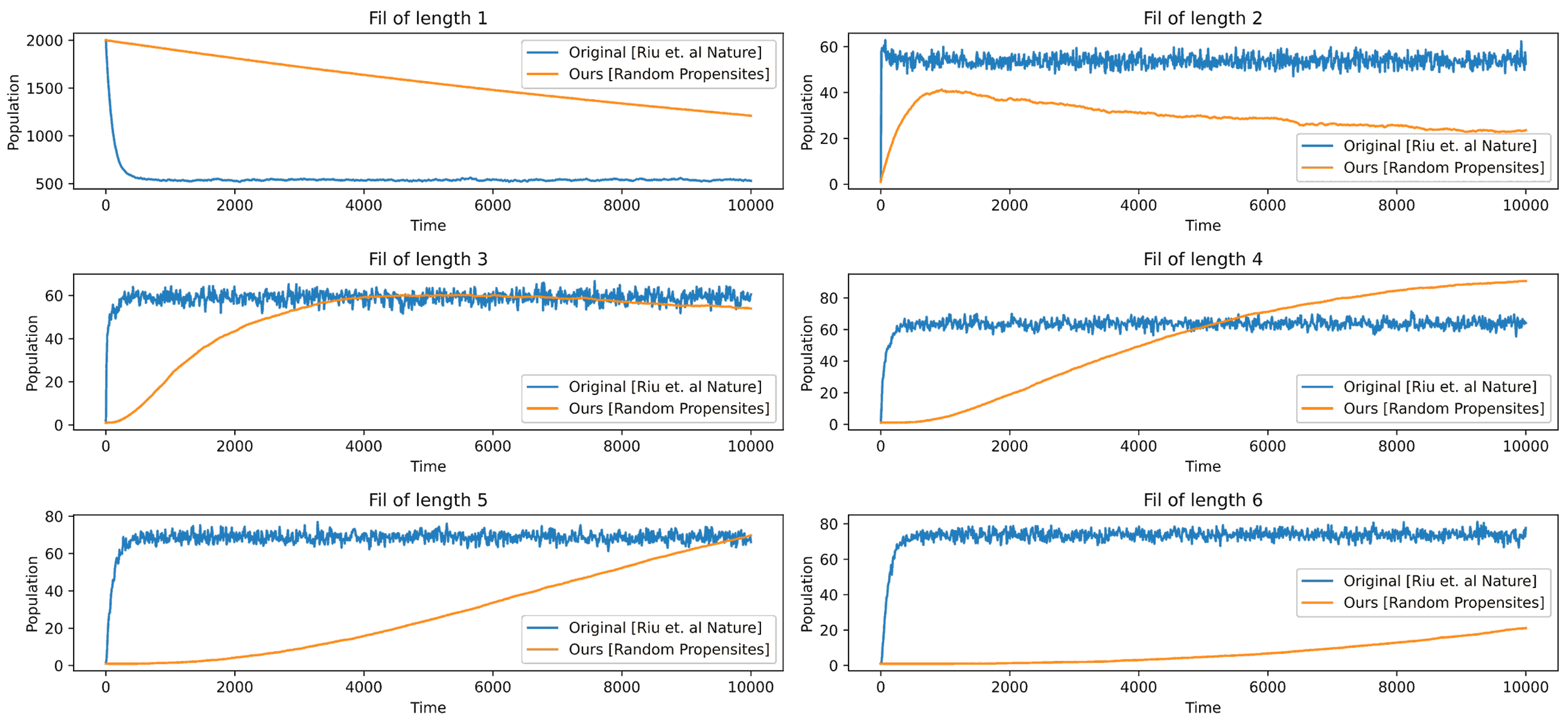
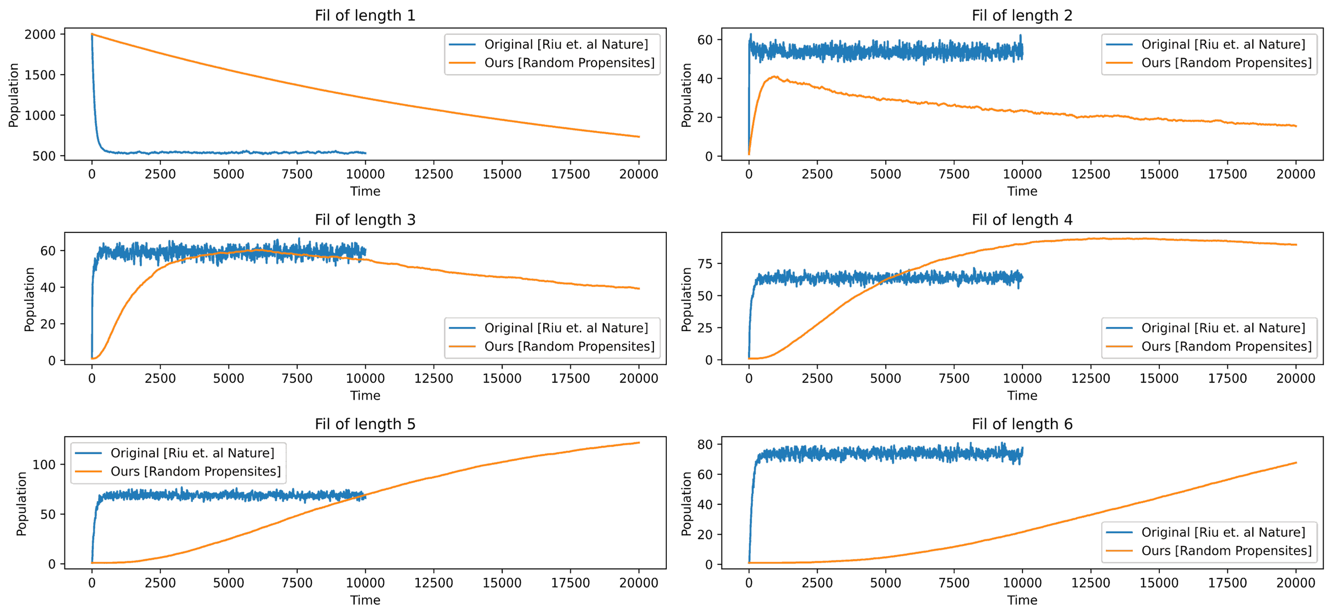
In Figure 12, we use random probabilities instead of the ones given in [13]. We can notice a sharp decline in the free protein, whereas ours has a gradual decline. Overall, the results are comparable, but one thing that we can instantly realize is that for our configuration to converge, we need to run the simulation for a longer time. In Figure 13, we run the simulation for longer time, and we can see that $M_2,M_3$, and $M_4$ first increase and then decrease. The highest convergence is in the filament of length six. The above results are obtained when we use their stoichiometry but using random propensities for the events instead of their fixed propensities. To produce these results, we use the starting probability or the probability of the occurrence of the first event elongation to be $0.0001$, then each subsequent event on the kinetics will have exactly half the probability than the one it preceded.

When we use our stoichiometry, which consists of 54 different possible reactions along with different propensities, although the filaments are not distributed comparably, their trajectories look similar. The result of this is given in the extra materials, the corresponding figures are Figures S7 and S8 of Supplementary Material.

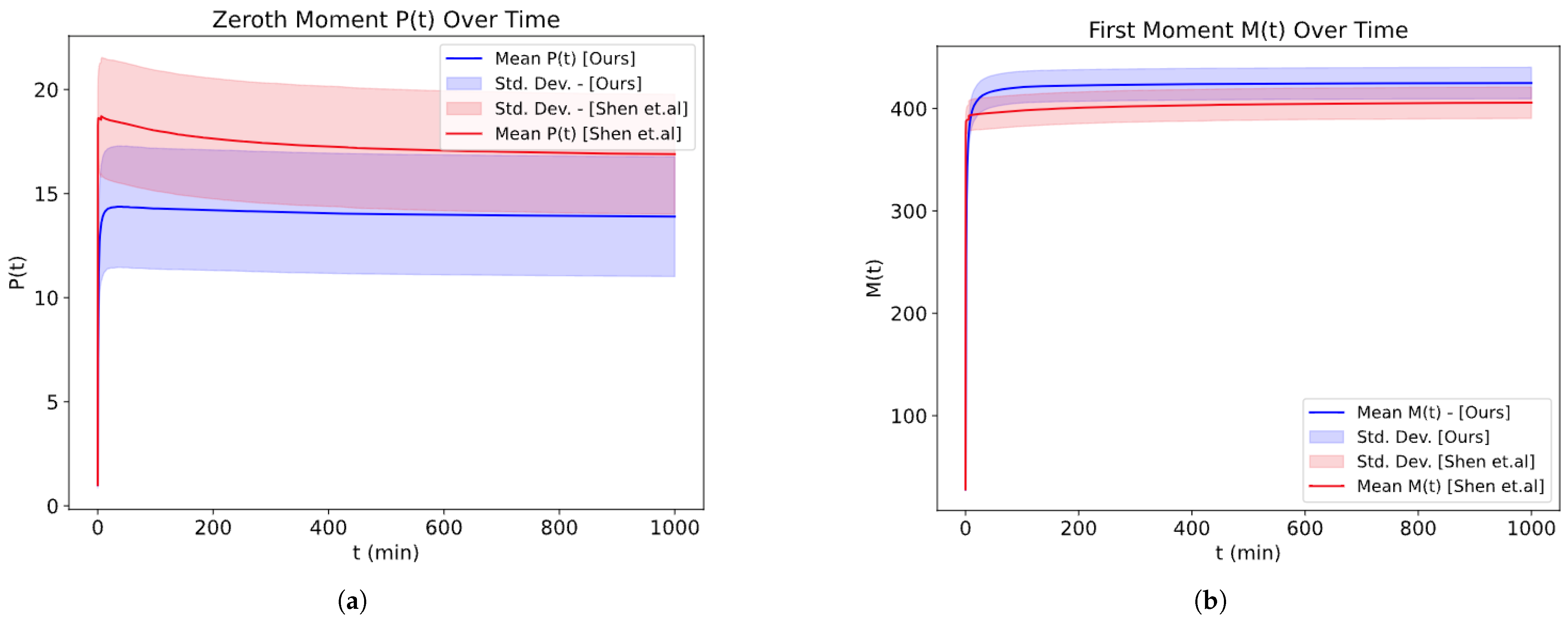
We further compare our work with [6], and as can be seen in Figure 14, we obtain a comparable result.

In Figure 14, there are two separate simulations: one uses the parameters of [6], whereas the other uses ours. Since [6] uses different units for time and the protein mass, we cannot compare them exactly, so we changed the parameters a little bit to make them comparable. Even though the probability used is not exactly the same, the output looks comparable in terms of convergence. However, it should be noted that we used our own stoichiometry matrix, as the author of [6] did not provide the stoichiometry used for their stochastic simulation.

5. Discussion and Results

5.1. Initial Conditions and System Dynamics

Our research delves into the complex interplay between the initial conditions and their eventual impact on system convergence. Specifically, the initial number of species serves as a critical determinant in shaping the system’s trajectory. This phenomenon is vividly illustrated in Figures S3–S6 of Supplementary Material. where varying the initial populations result in distinct convergence patterns. Notably, initial populations of 1 and 5 yield similar convergence behaviors, but a shift to 10 aligns the convergence pattern more closely with that observed at an initial population of 100. This shift underscores a nonlinear relationship between the initial population sizes and system behavior, suggesting a threshold effect, where beyond a certain population size, the system dynamics alter significantly.

5.2. Role of Reaction Rates in System Convergence

When exploring the influence of constant reaction rates on the system, especially in the context of primary nucleation (as seen in Figures S4 and S5 of Supplementary Material, we observe a reduced rate of convergence. This finding indicates the sensitivity of the system to the reaction rate parameters, emphasizing the importance of these parameters in predictive modeling. The consistency of the final convergence at filament length six across various scenarios also points to an inherent bias in the system towards certain states. The predominance of specific reaction events—namely, primary nucleation, elongation, and aggregation with monomer-dependent secondary nucleation—suggests an intrinsic propensity of the system towards these pathways. While the higher probability of primary nucleation is expected, the regular occurrence of monomer-dependent secondary nucleation and aggregation in every simulation warrants further examination to uncover the underlying mechanisms.

5.3. Impact of Secondary Events and Random Variability

Another notable finding is the minimal impact of secondary events, such as fragmentation, on the final convergence of the filament lengths. Conversely, introducing random variations in the probability of different reaction events significantly altered the final convergence as illustrated in Figure 9. Interestingly, even with this randomness, reactions predominantly converged towards $M_6$. This could suggest the dominance of certain events over others. The extent of change in convergence was directly proportional to the probability of these random switches; a higher probability led to a lower final $P\left(t\right)$ and $M\left(t\right)$, but as this probability approached zero, its impact diminished.

5.4. Statistical Consistency and Determinism in Stochastic Simulations

Our aggregation and analysis of reaction events across multiple simulations revealed a statistically consistent pattern, with primary nucleation, elongation, and aggregation with monomer-dependent secondary nucleation being the most frequent. This consistency, even in the face of stochastic variability, highlights an underlying determinism in the system. The results of 100 Monte Carlo simulations further strengthen this notion, showing minimal variation in the population of different filament lengths.

5.5. Comparison with Other Studies

A crucial aspect of our study is the comparison of our stochastic simulation results with established models in the field, specifically those reported in [6,13]. This comparison validated our findings, indicating a close alignment between the outcomes of our stochastic simulations and those derived from not only from stochastic models, but also from deterministic models like the moment closure method [13] and the second-stochastization method [6]. Such validation not only reinforces the reliability of our methods but also contributes to a deeper understanding of the dynamic behaviors of biological systems under varying conditions.

5.6. Limitations and Future Works

While our research provided valuable insights, it is important to recognize certain constraints that frame our findings. One notable limitation is the absence of realistic numbers of soluble protein extended-duration simulations. Ideally, longer simulations would offer a more realistic representation of the biological processes under study. However, the substantial computational resources required for such extensive kinetic simulations of reaction processes pose a significant challenge. We anticipate addressing this aspect in future research, leveraging advancements in computational capabilities to explore longer timeframes. Another area that was not within the ambit of our current investigation is the mathematical analysis of the system’s stability and convergence. While this analytical approach was beyond the scope of our present work, it represents a promising avenue for future exploration. A mathematical framework could provide a deeper understanding of the underlying dynamics and enhance the predictive power of our models. Furthermore, a direct comparison of our simulation results with experimental data would have enriched our study. Unfortunately, challenges in accessing relevant experimental data limited our ability to perform this comparison. Moving forward, we aim to integrate empirical data into our analysis, as this would not only validate our simulation results but also offer a more comprehensive perspective on the biological phenomena we are examining.

6. Conclusions

Our study underscores the crucial role of stochastic modeling in capturing the nuances of biological processes, particularly in scenarios where deterministic models fall short. Deterministic approaches, while effective in representing the average dynamics of macroscopic experiments, often fail to encapsulate the inherent stochastic fluctuations that are especially pronounced in microscopic cellular processes. To bridge this gap, we employed stochastic modeling to simulate the dynamics of amyloid-beta aggregation in Alzheimer’s disease, a process fraught with randomness and complexity. The findings from our stochastic models yielded significant insights. We observed that the evolution of amyloid-beta filaments of varying lengths is intricately tied to the specific reaction rates employed in the model. This link underscores the sensitivity of the aggregation process to these rates, paving the way for a deeper understanding of the mechanisms driving amyloid-beta aggregation.

A particularly striking observation is the tendency of the system to converge towards filaments of a specific length, in our case, length six. This convergence suggests a dominance of certain reaction events over others, an aspect that could be pivotal in understanding the progression of Alzheimer’s disease at a molecular level. Moreover, the influence of reaction probabilities on the system’s final convergence and stability was evident, reinforcing the importance of these parameters in the aggregation process. Additionally, our exploration of random reaction propensities revealed marked differences in convergence patterns, highlighting the impact of stochastic variability on the system’s behavior. This aspect of our study points to the potential of stochastic models to reveal subtleties that deterministic models might overlook.

In conclusion, our comprehensive stochastic simulations not only enhance our current understanding of amyloid-beta aggregation but also set the stage for future research. They open new avenues for employing sophisticated stochastic modeling techniques to unravel the intricate dynamics of amyloid-beta aggregation. This comprehensive simulation could be instrumental in understanding and developing more effective strategies for combating diseases, such as Alzheimer’s, which are directly or indirectly related to the protein aggregation process by providing a more detailed understanding of the underlying molecular processes.

References

1. 2023 Alzheimer’s disease facts and figures. Alzheimer’s Dement. 2023, 19, 1598–1695. [CrossRef]
2. Gauthier, S.; Webster, C.; Servaes, S.; Morais, J.A.; Rosa-Neto, P. World Alzheimer Report 2022: Life after Diagnosis: Navigating Treatment, Care and Support; Alzheimer’s Disease International: London, UK, 2022. [Google Scholar]
3. Knopman, D.S. The Initial Recognition and Diagnosis of Dementia. Am. J. Med. 1998, 104, 2S–12S. [Google Scholar] [CrossRef]
4. Dementia Statistics|Alzheimer’s Disease International (ADI). Available online: https://www.alzint.org/about/dementia-facts-figures/dementia-statistics/ (accessed on 25 June 2023).
5. Finder, V.H. Alzheimer’s Disease: A General Introduction and Pathomechanism. J. Alzheimer’s Dis. 2010, 22, S5–S19. [Google Scholar]
6. Shen, J.L.; Tsai, M.Y.; Schafer, N.P.; Wolynes, P.G. Modeling Protein Aggregation Kinetics: The Method of Second Stochasticization. J. Phys. Chem. B 2021, 125, 1118–1133. [Google Scholar] [CrossRef]
7. Lukiw, W.J. Amyloid beta (Aβ) peptide modulators and other current treatment strategies for Alzheimer’s disease (AD). Expert Opin. Emerg. Drugs 2012, 17, 43–60. [Google Scholar] [CrossRef]
8. Demetrius, L.A.; Magistretti, P.J.; Pellerin, L. Alzheimer’s disease: The amyloid hypothesis and the Inverse Warburg effect. Front. Physiol. 2015, 5, 522. [Google Scholar] [CrossRef]
9. Knowles, T.P.J.; Waudby, C.A.; Devlin, G.L.; Cohen, S.I.A.; Aguzzi, A.; Vendruscolo, M.; Terentjev, E.M.; Welland, M.E.; Dobson, C.M. An Analytical Solution to the Kinetics of Breakable Filament Assembly. Science 2009, 326, 1533–1537. [Google Scholar] [CrossRef]
10. Hardy, J. Alzheimer’s disease: The amyloid cascade hypothesis: An update and reappraisal. J. Alzheimer’s Dis. 2006, 9, 151–153. [Google Scholar]
11. Braak, H.; Del Tredici, K. Neurofibrillary Tangles. In Encyclopedia of Movement Disorders; Kompoliti, K., Metman, L.V., Eds.; Academic Press: Oxford, UK, 2010; pp. 265–269. [Google Scholar] [CrossRef]
12. Carradori, D.; Gaudin, A.; Brambilla, D.; Andrieux, K. Chapter Three—Application of Nanomedicine to the CNS Diseases. In Nanotechnology and the Brain; Al-Jamal, K.T., Ed.; International Review of Neurobiology; Academic Press: Cambridge, MA, USA, 2016; Volume 130, pp. 73–113. [Google Scholar] [CrossRef]
13. Liu, R.N.; Kang, Y.M. Stochastic master equation for early protein aggregation in the transthyretin amyloid disease. Sci. Rep. 2020, 10, 12437. [Google Scholar]
14. Cohen, S.I.A.; Vendruscolo, M.; Welland, M.E.; Dobson, C.M.; Terentjev, E.M.; Knowles, T.P.J. Nucleated polymerization with secondary pathways. I. Time evolution of the principal moments. J. Chem. Phys. 2011, 135, 065105. [Google Scholar] [CrossRef]
15. Hadjichrysanthou, C.; Ower, A.K.; de Wolf, F.; Anderson, R.M.; for the Alzheimer’s Disease Neuroimaging Initiative. The development of a stochastic mathematical model of Alzheimer’s disease to help improve the design of clinical trials of potential treatments. PLoS ONE 2018, 13, e0190615. [Google Scholar] [CrossRef]
16. Atlante, A.; de Bari, L.; Bobba, A.; Amadoro, G. A disease with a sweet tooth: Exploring the Warburg effect in Alzheimer’s disease. Biogerontology 2017, 18, 301–319. [Google Scholar] [CrossRef]
17. Traxler, L.; Herdy, J.R.; Stefanoni, D.; Eichhorner, S.; Pelucchi, S.; Szücs, A.; Santagostino, A.; Kim, Y.; Agarwal, R.K.; Schlachetzki, J.C.; et al. Warburg-like metabolic transformation underlies neuronal degeneration in sporadic Alzheimer’s disease. Cell Metab. 2022, 34, 1248–1263.e6. [Google Scholar] [CrossRef]
18. Chen, G.-F.; Xu, T.-H.; Yan, Y.; Zhou, Y.-R.; Jiang, Y.; Melcher, K.; Xu, H.E. Amyloid beta: Structure, biology and structure-based therapeutic development. Acta Pharmacol. Sin. 2017, 38, 1205–1235. [Google Scholar] [CrossRef]
19. Sontheimer, H. Chapter 4—Aging, Dementia, and Alzheimer Disease. In Diseases of the Nervous System; Sontheimer, H., Ed.; Academic Press: San Diego, CA, USA, 2015; pp. 99–131. [Google Scholar] [CrossRef]
20. Meyer, R. Beta Amyloid. In xPharm: The Comprehensive Pharmacology Reference; Enna, S., Bylund, D.B., Eds.; Elsevier: New York, NY, USA, 2008; pp. 1–3. [Google Scholar] [CrossRef]
21. Weller, R.; Carare, R.; Boche, D. Amyloid: Vascular and Parenchymal. In Reference Module in Neuroscience and Biobehavioral Psychology; Elsevier: Amsterdam, The Netherlands, 2017. [Google Scholar] [CrossRef]
22. Valasani, K.; Carlson, E.; Vangavaragu, J.; Yan, S. Chapter 10—Mitochondria as a Therapeutic Target for the Treatment of Alzheimer’s Disease. In Drug Discovery Approaches for the Treatment of Neurodegenerative Disorders; Adejare, A., Ed.; Academic Press: Cambridge, MA, USA, 2017; pp. 195–209. [Google Scholar] [CrossRef]
23. Bianca Velasco, A.; Tan, Z.S. Chapter 17—Fatty Acids and the Aging Brain. In Omega-3 Fatty Acids in Brain and Neurological Health; Watson, R.R., De Meester, F., Eds.; Academic Press: Boston, MA, USA, 2014; pp. 201–219. [Google Scholar] [CrossRef]
24. Amyloid Plaques and Neurofibrillary Tangles|BrightFocus Foundation. Available online: https://www.brightfocus.org/news/amyloid-plaques-and-neurofibrillary-tangles (accessed on 9 July 2023).
25. Cacabelos, R.; Cacabelos, P.; Torrellas, C. Chapter 27—Personalized Medicine of Alzheimer’s Disease. In Handbook of Pharmacogenomics and Stratified Medicine; Padmanabhan, S., Ed.; Academic Press: San Diego, CA, USA, 2014; pp. 563–615. [Google Scholar] [CrossRef]
26. Martinez-Torres, C.; Burla, F.; Alkemade, C.; Koenderink, G.H. Revealing the assembly of filamentous proteins with scanning transmission electron microscopy. PLoS ONE 2019, 14, e0226277. [Google Scholar] [CrossRef]
27. Muñoz-Lasso, D.C.; Romá-Mateo, C.; Pallardó, F.V.; Gonzalez-Cabo, P. Much More Than a Scaffold: Cytoskeletal Proteins in Neurological Disorders. Cells 2020, 9, 358. [Google Scholar] [CrossRef]
28. Cytoskeleton Filaments—Physiopedia. Available online: https://www.physio-pedia.com/Cytoskeleton_Filaments#cite_note-5 (accessed on 10 July 2023).
29. Gillespie, D.T. A general method for numerically simulating the stochastic time evolution of coupled chemical reactions. J. Comput. Phys. 1976, 22, 403–434. [Google Scholar] [CrossRef]
30. Loof, A.D.; Schoofs, L. Alzheimer’s Disease: Is a Dysfunctional Mevalonate Biosynthetic Pathway the Master-Inducer of Deleterious Changes in Cell Physiology? OBM Neurobiol. 2019, 3, 046. [Google Scholar] [CrossRef]
31. Feinberg, M. Foundations of Chemical Reaction Network Theory; Springer: Cham, Switzerland, 2019. [Google Scholar]
32. Qian, H.; Ge, H. Stochastic Chemical Reaction Systems in Biology; Springer: Cham, Switzerland, 2021. [Google Scholar]
33. Schuster, P. Stochasticity in Processes; Springer: Cham, Switzerland, 2016. [Google Scholar]
34. Cohen, S.I.; Vendruscolo, M.; Dobson, C.M.; Knowles, T.P. Nucleated polymerization with secondary pathways. II. Determination of self-consistent solutions to growth processes described by non-linear master equations. J. Chem. Phys. 2011, 135, 08B611. [Google Scholar]
35. Oosawa, F.; Asakura, S. Thermodynamics of the Polymerization of Protein; Academic Press: London, UK, 1975. [Google Scholar]
36. Rukmangadachar, L.A.; Bollu, P.C. Amyloid Beta Peptide. In StatPearls; StatPearls Publishing: Treasure Island, FL, USA, 2023. [Google Scholar]
37. Silva, M.V.F.; Loures, C.d.M.G.; Alves, L.C.V.; de Souza, L.C.; Borges, K.B.G.; Carvalho, M.d.G. Alzheimer’s disease: Risk factors and potentially protective measures. J. Biomed. Sci. 2019, 26, 33. [Google Scholar] [CrossRef]
Figure 1. The presence of amyloid plaques and neurofibrillary tangles in the AD-infected brain versus the normal human brain. Figure motivated from [24].
Processes 12 00157 g001
Figure 2. Schematic representation of the microscopic processes of A β fibril formation and elongation.
Processes 12 00157 g002
Figure 3. The evolution of amyloid beta aggregations, Condition 1 with the initial population of free proteins M 1 = 10 , 000 , and Condition 2 with the initial population of free proteins M 1 = 5000 . The initial condition for each population except M 1 is the same, 100 , 60 , 50 , 20 , 10 , 5 , 5 for M 2 , M 3 , , M 8 , respectively. The starting reaction rate k 0 = 0.00001 .
Processes 12 00157 g003aProcesses 12 00157 g003b
Figure 4. The evolution of amyloid-beta aggregations, Condition 1 with the initial population of free proteins M 1 = 10 , 000 , and Condition 2 with the initial population of free proteins M 1 = 5000 . The initial condition for each population except M 1 is the same, 1 , 1 , 1 , 1 , 1 , 1 , 1 for M 2 , M 3 , , M 8 , respectively. The starting reaction rate k 0 = 0.00001 .
Processes 12 00157 g004aProcesses 12 00157 g004b
Figure 5. The evolution of amyloid-beta aggregations and fragmentation when the rate constants are different for different reactions, e.g., k 0 , , k 53 are different, Condition 1 with the initial population of free proteins M 1 = 10,000 , and Condition 2 with the initial population of free proteins M 1 = 5000 . The initial condition for each population except M 1 is the same, 100 , 100 , 100 , 100 , 100 , 100 , 100 for M 2 , M 3 , , M 8 , respectively. The starting reaction rate k 0 = 0.00001 for aggregation and starting rate for fragmentation k 1 = 0.00001 / 2 .
Processes 12 00157 g005aProcesses 12 00157 g005b
Figure 6. The evolution of amyloid-beta aggregations and fragmentation when the rate constants are different for different reactions, e.g., k 0 , , k 53 are different, Condition 1 with the initial population of free proteins M 1 = 10,000 and Condition 2 with the initial population of free proteins M 1 = 5000 . The initial condition for each population except M 1 is the same, 1 , 1 , 1 , 1 , 1 , 1 , 1 for M 2 , M 3 , , M 8 , respectively. The starting reaction rate k 0 = 0.00001 for fragmentation and starting rate for fragmentation k 1 = 0.00001 / 2 .
Processes 12 00157 g006aProcesses 12 00157 g006bProcesses 12 00157 g006c
Figure 7. The evolution of amyloid-beta aggregations and fragmentation when the rate constants are constant for all reactions except from k 0 = 0.0000001 , e.g., k 1 , , k 26 = 0.0000000002 and k 27 , k 53 = 0.0000000002 / 2 ; Condition 1 with the initial population of free proteins M 1 = 10,000 ; and Condition 2 with the initial population of free proteins M 1 = 5000 . The initial condition for each population except M 1 is the same, 100 , 100 , 100 , 100 , 100 , 100 , 100 for M 2 , M 3 , , M 8 , respectively.
Processes 12 00157 g007aProcesses 12 00157 g007bProcesses 12 00157 g007c
Figure 8. The evolution of amyloid-beta aggregations and fragmentation events and their occurrence dynamics with different initial conditions and reaction rates. The average reaction dynamics corresponding to Figure 5, with M 1 = 10 , 000 and M 2 , , M 8 = 100 .
Processes 12 00157 g008
Figure 9. Comparison of P(t) and M(t) with and without random switching of probability. (a) The zeroth moment P(t) over time, all constants are same as in Figure 4. (b) The zeroth moment P(t) over time with random probability switching, all constants are the same as in Figure 4. (c) The first moment M(t) over time, all constants are the same as in Figure 4. (d) The first moment M(t) over time with random probability switching, all constants are same as in Figure 4. (e) The zeroth moment P(t) over time, all constants are same as in Figure 6. (f) The zeroth moment P(t) over time with random probability switching, all constants are same as in Figure 6. (g) The first moment M(t) over time, all constants are same as in Figure 6. (h) The first moment M(t) over time with random probability switching, all constants are same as in Figure 6.
Processes 12 00157 g009aProcesses 12 00157 g009b
Figure 10. The evolution of amyloid-beta aggregations and fragmentation events and their occurrence dynamics with different initial conditions and reaction rates. The average reaction dynamics with M 1 = 10 , 000 and M 2 , , M 8 = 1 and random switching with dynamic constant rates as in Figure 6.
Processes 12 00157 g010
Figure 11. The phase diagrams of zeroth moment P(t) and first moment M(t) over time using same initial population but different reaction probabilities. (a) The phase diagram of P(t), M(t) over time using initial condition M 1 = 5000 and M 2 , , M 8 = 1 and constant rates as in Figure 6. (b) The phase diagram of P(t), M(t) over time using initial condition M 1 = 5000 and M 2 , , M 8 = 1 and constant rates as in Figure 7.
Processes 12 00157 g011
Figure 12. The evolution of different lengths of the filaments, one in the configuration of [13] and the other in our configuration. The M 0 here is 2000, and the time end is 10,000 s.
Processes 12 00157 g012
Figure 13. The evolution of different lengths of the filaments, one in the configuration of [13] and the other in our configuration. The M 0 here is 2000, and the time end is 10,000 and 20,000 s, respectively.
Processes 12 00157 g013
Figure 14. Comparison of stochastic simulation of [6] and ours. (a) Comparison of zeroth moment P ( t ) of aggregation of filaments with [6]: the red color denotes the reproduction of [6] and blue color represents our simulation. The initial population of free proteins M 1 = 500 and the time end 1000. (b) Comparison of first moment M ( t ) of aggregation of filaments with [6]: the red color denotes the reproduction of [6] and the blue color represents our simulation. The initial population of free proteins is M 1 = 500 , and the time end is 1000.
Processes 12 00157 g014