Abstract
The bottomhole pressure is one of the key parameters for oilfield development and decision-making. However, due to factors such as cost and equipment failure, bottomhole pressure data is often lacking. In this paper, we established a GA-XGBoost model to predict the bottomhole pressure in carbonate reservoirs. Firstly, a total of 413 datasets, including daily oil production, daily water production, daily gas production, daily liquid production, daily gas injection rate, gas–oil ratio, and bottomhole pressure, were collected from 14 wells through numerical simulation. The production data were then subjected to standardized preprocessing and dimensionality reduction using a principal component analysis. The data were then split into training, testing, and validation sets with a ratio of 7:2:1. A prediction model for the bottomhole pressure in carbonate reservoirs based on XGBoost was developed. The model parameters were optimized using a genetic algorithm, and the average adjusted R-squared score from the cross-validation was used as the optimization metric. The model achieved an adjusted R-squared score of 0.99 and a root-mean-square error of 0.0015 on the training set, an adjusted R-squared score of 0.84 and a root-mean-square error of 0.0564 on the testing set, and an adjusted R-squared score of 0.69 and a root-mean-square error of 0.0721 on the validation set. The results demonstrated that in the case of fewer data variables, the GA-XGBoost model had a high accuracy and good generalization performance, and its performance was superior to other models. Through this method, it is possible to quickly predict the bottomhole pressure data of carbonate rocks while saving measurement costs.
1. Introduction
The bottomhole pressure is one of the key parameters for oilfield development and decision-making. The difference between the bottomhole pressure and the formation pressure largely determines the oil production rate of a well. Traditional methods of obtaining the bottomhole pressure include installing downhole pressure sensors for measurement, a well-testing analysis, or establishing numerical simulation models. The installation of pressure gauges for all wells is costly and carries risks such as equipment lifespan and failures, leading to expensive workovers for equipment replacement and production delays. Well-testing methods also require well shutdowns, which affect economic benefits and involve complex operations. Numerical simulation methods are time-consuming, labor-intensive, and resource-demanding. Therefore, it is crucial to develop a real-time pressure prediction model that saves time, effort, and costs in order to continuously and accurately obtain the bottomhole pressure without shutting down the wells. The traditional correlation prediction methods for forecasting the bottomhole pressure rely on the establishment of empirical and semiempirical (mechanistic) models. Studies by Duns and Ros [1], Hagedorn and Brown [2], Orkiszewski [3], and Beggs and Brill [4] have focused on empirical models, while Mukherjee and Brill [5], Ansari et al. [6], Chokshi et al. [7], and Gomez et al. [8] have researched semi-empirical (mechanistic) models. However, these methods are largely based on a series of specific conditions. Therefore, when applied beyond these conditions, the effectiveness of these methods deteriorates.
Artificial intelligence (AI) has a strong adaptability and flexibility in various environments and datasets, and is widely used in fields such as medicine, transportation, the Internet, and energy. In the application of petroleum engineering, AI is often used to solve problems related to data, optimization, identification, and knowledge integration [9,10]. AI technology can more accurately predict bottomhole pressure by learning patterns and correlations from a large quantity of historical data (as shown in Table 1), especially in complex reservoir conditions and dynamic oilfield development processes. Awadalla and Yousef (2016) [11] used backpropagation algorithm to find the optimal parameters of a feedforward neural network (FFNN) for predicting the bottomhole flowing pressure of vertical oil wells. Mahshid and Suren (2019) [12] predicted the bottomhole flowing pressure of coalbed methane wells using time data, linear regression, and neural-network-based methods. Ahmadi and Chen (2019) [13] compared various artificial neural network methods for predicting the bottomhole pressure of vertical wells, and the results showed that a hybrid genetic algorithm and particle swarm optimization (HGAPSO) was highly accurate. Nait Amar et al. (2018) [14] demonstrated that a hybrid model based on artificial neural network (ANN) and grey wolf optimization (GWO) (ANN-GWO) performed better than other hybrid methods such as genetic algorithm (GA), particle swarm optimization (PSO), or using only a BPNN (backpropagation neural network). Nait Amar and Zeraibi (2020) [15] proposed a hybrid model based on support vector regression (SVR) and the firefly algorithm (FFA) for predicting the bottomhole pressure (BHP) in vertical wells under multiphase flow conditions. Rathnayake et al. (2022) [16] compared multiple linear regression, linear mixed effects, and gradient boosting regression tree (XGBoost) methods for predicting the flowing bottomhole pressure (FBHP) in gas wells, and the results showed that the XGBoost method had the best prediction results.

Table 1.
Summary of artificial intelligence algorithms for bottomhole pressure prediction.
Based on previous research, this study proposes a well bottom-pressure prediction model based on XGBoost. The XGBoost algorithm [21] is an ensemble learning algorithm based on gradient boosting trees, which has been widely applied in various fields such as healthcare [22] and telecommunications [23] and has been introduced in several articles regarding its application in the petroleum field. For example, Pan et al. applied XGBoost to predict porosity in well logging [24]; Markovic et al. applied XGBoost to predict water saturation in rock physics [25]; Zhong et al. used XGBoost to generate pseudodensity logging data [26]; Gu et al. applied it to predict permeability in geology [27]; Al Mudhafar et al. applied XGBoost to the reservoir lithology classification of carbonate rocks [28]; Zhang et al. applied it to predict hydrocarbon gases in petrochemistry [29]; Dong et al. used XGBoost for reservoir production prediction [30]; and Wang et al. applied XGBoost to predict reservoir production in highly heterogeneous sandstone [31]. These applications have demonstrated that XGBoost is an efficient, superior, and reliable algorithm. Compared with traditional machine learning algorithms, XGBoost exhibits a higher accuracy, greater flexibility, and is less prone to overfitting, demonstrating significant advantages in large-scale, efficient, and accurate problems. However, there is almost no application of XGBoost in well bottom-pressure prediction in carbonate reservoirs.
One major issue faced by machine learning models, including XGBoost, is the close relationship between the model’s performance and its hyperparameters. Using default parameter values may not fully harness the powerful effects of XGBoost. Conventional grid-search algorithms require manual parameter tuning, which consumes a lot of time and effort and makes finding the global optimal value challenging. The enhanced elite strategy genetic algorithm is an improved genetic algorithm that can more easily find the global optimal solution. Therefore, this paper proposes the use of an improved genetic algorithm to optimize the hyperparameters of XGBoost in order to enhance the prediction accuracy and generalization performance of the XGBoost model. The data used in this study were production data collected from a numerical model fitted to the historical data of the X oilfield. Prior to establishing the XGBoost-based prediction model for carbonate reservoir bottomhole pressure, various preprocessing steps such as data correlation analysis and data dimensionality reduction were conducted. The optimized XGBoost model with adjusted hyperparameters was compared with ten other machine learning models, namely, support vector machines, neural networks, stochastic gradient descent, linear regression, ridge regression, decision trees, random forests, gradient boosting trees, ExtraTrees, and Adaboost, to evaluate the superior predictive performance of XGBoost. These models were selected due to their frequent utilization in machine learning problems. The novelty of this work compared to other studies in the field lies in the following aspects: (1) The X oilfield is a matrix-pore-type carbonate reservoir with localized fractures and dissolution cavities, as well as high-permeability streaks and impermeable interlayers, exhibiting an extremely strong heterogeneity. The uneven pressure distribution during the development process poses a significant challenge for pressure prediction. The use of numerical simulation for pressure prediction requires a great deal of work, and there is currently no suitable empirical formula for pressure prediction in this type of oilfield. Using XGBoost through data-driven methods for pressure prediction is a relatively feasible approach. (2) Previous research often involves collecting extensive geological, development, engineering, well logging, and seismic data to achieve optimal machine learning results. However, due to the inconvenience of a practical application caused by the need for extensive data collection, this work utilizes only six easily collectible production data variables (daily oil production, daily water production, daily gas production, daily liquid production, daily gas injection, and gas–oil ratio) to test the performance of the model in the case of limited data variables. The utilization of a smaller set of variables in model training also facilitates the rapid implementation of real-time bottomhole pressure prediction in the field. (3) The model compares the pressure prediction performance of ten different machine learning algorithms with that of GA-XGBoost, demonstrating the superior accuracy and generalization ability of XGBoost in pressure prediction problems with limited data variables. This workflow also has certain limitations, as the data used are derived from numerical simulations. Although the model has undergone historical fitting, there are still errors compared to actual production data.
2. Principles and Methods
2.1. The Principles of the XGBoost Method
XGBoost [21] is an ensemble algorithm that combines multiple weak classifiers into a strong classifier based on the decision tree algorithm. It enhances the accuracy of predictive models by constructing multiple CART decision trees. The final prediction is obtained by summing the predictions of each trained decision tree in each round of training.
The principle of the XGBoost algorithm is as follows [32]:
In the equation, represents the number of trees in the model. denotes a function in the function space . represents the predicted value, and represents the i-th input data. represents the set of all possible CART models.
At each iteration, the model remains unchanged, and a new function is added to the existing model. Each function corresponds to a tree, and the newly generated tree is used to fit the residual of the previous prediction. The iterative process is as follows:
The objective function of XGBoost is as follows [33]:
In Equation (3), is used to measure the discrepancy between predicted scores and true scores, and is the regularization term that effectively prevents overfitting. In Equation (4), represents the number of leaf nodes, represents the score of each leaf node, is used to control the number of leaf nodes, and ensures that the scores of leaf nodes are not too large.
XGBoost has several main parameters that need to be adjusted: the number of sub-models, the learning rate, the maximum depth, the minimum child weight, , the subsample rate, and the column sampling rate. These hyperparameters affect the final performance of the model but in different ways. Therefore, it is necessary to optimize these hyperparameters.
2.2. Genetic Algorithm
Genetic algorithms (GAs) have been proven to be superior to traditional methods when performing a global search within a complex search space [34]. Usually starting from a group of randomly generated candidates embedded with potential solutions, a GA creates a new generation in each iteration by transferring crucial information such as survival of the fittest, crossover, and mutation operations onto promising candidates selected based on the probability biased towards relatively fitter agents [35].
The enhanced elite retention strategy for genetic algorithm (SEGA) takes advantage of the best individuals (called elites) generated during evolution, which are not subjected to selection, crossover, and mutation but directly copied to the next generation. The main feature of this operation is that elites produced during evolution will not be lost or damaged due to pairing crossover and other operations, significantly improving the ability to reach global convergence.
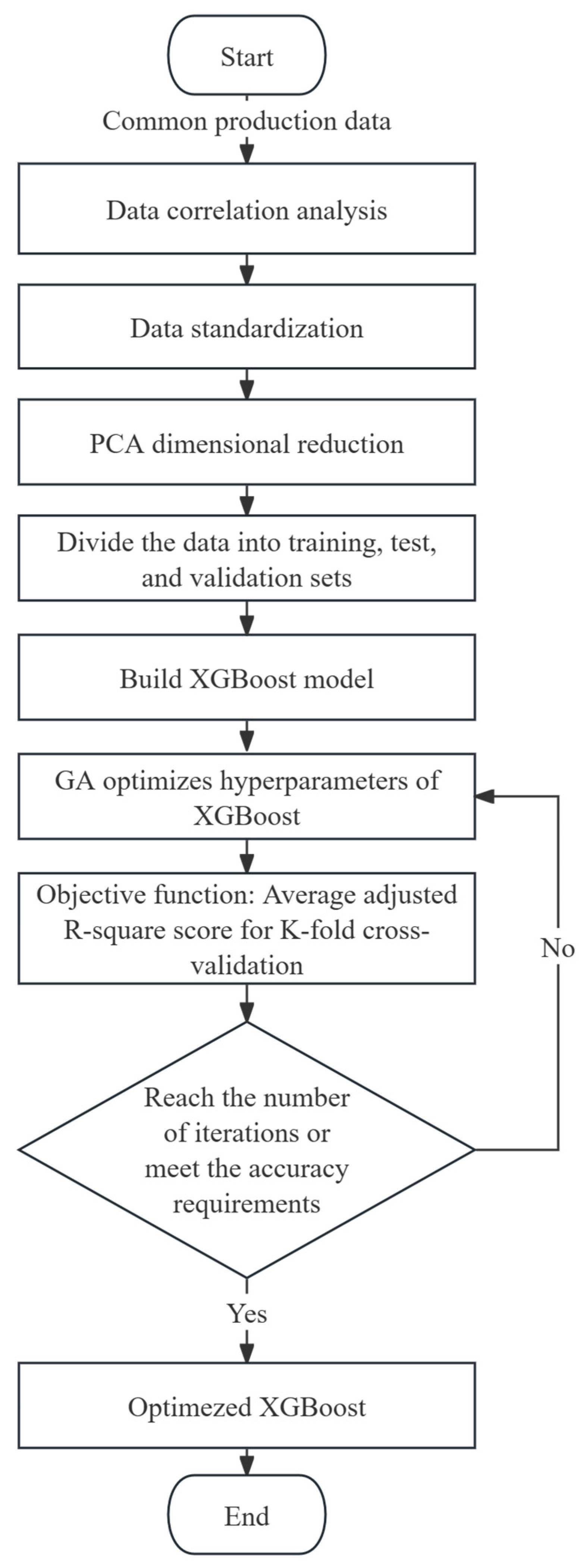
This paper utilizes the SEGA (Sequential Evolutionary Grid Algorithm) to continuously optimize the parameters of XGBoost and achieve the maximum cross-validation adjusted R-squared score, thereby accurately predicting the bottomhole pressure. The SEGA initially generates a batch of XGBoost hyperparameter initial values within a specified range and trains them with production data from the reservoir to obtain a score for the bottomhole pressure prediction. A higher score indicates better model performance. Based on the objective of maximizing the score, the elite preservation strategy is employed to generate the next generation of superior XGBoost hyperparameter populations, which are then trained to obtain scores. This process continues until the maximum evolution generation or the optimization objective reaches a predetermined threshold. The model training process is illustrated in Figure 1. By utilizing this method, the SEGA automatically searches for the optimal parameters of the XGBoost model. Compared to conventional grid-search methods, it eliminates the need for exhaustive parameter exploration, resulting in faster optimization speed, lower computational cost, and significant time and effort savings.
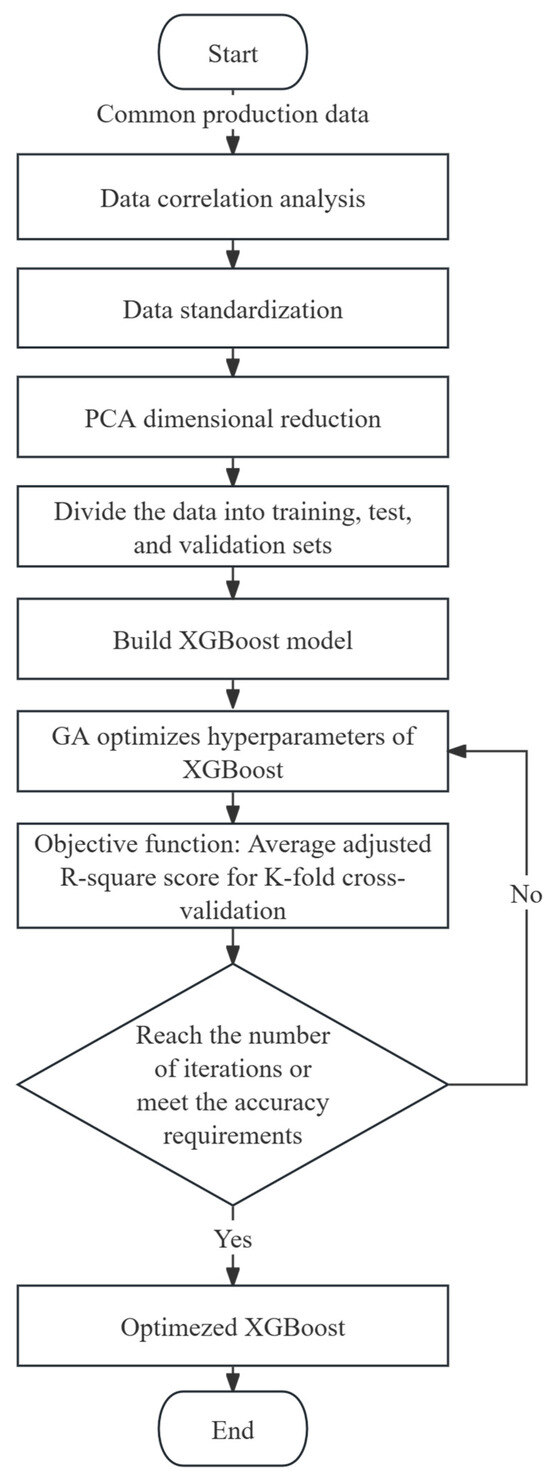
Figure 1.
GA-XGBoost model flow diagram.
3. Model Verification and Application
The numerical simulation, through historical fitting, can represent, to some extent, the actual conditions of the target oilfield. The numerical model of the target oilfield had a grid size of 300 × 300 × 20 m, with a total of 239,000 effective grid cells. The boundaries were closed on all sides, and there were 8 components in the model. The model simulation parameters are shown in Table 2. Based on the actual production data and pressure test data, the fitting of a fixed oil volume and single well pressure was carried out, and the overall fitting effect was good.
Table 2.
Model parameters.
Common production data (daily oil production, daily water production, daily gas production, daily liquid production, daily gas injection rate, gas–oil ratio, and bottomhole pressure) were collected from the numerical model as the dataset. The bottomhole flowing pressure was treated as the target value, while the remaining data served as input values.
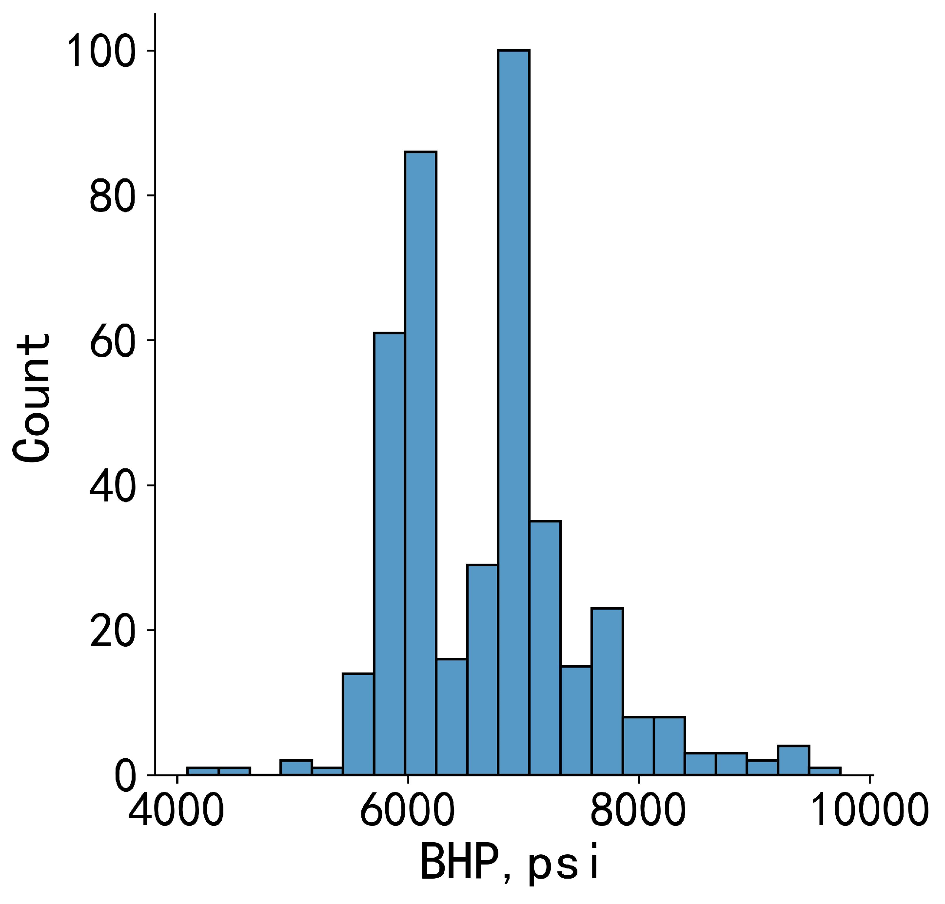
A total of 413 datasets were collected from 14 wells. It can be observed from Figure 2, the distribution of the bottomhole pressure was uneven, mainly concentrated in the area of 5500 psi to 8300 psi, with the most data distributed around 7000 psi.
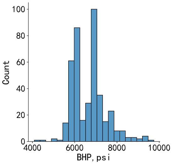
Figure 2.
Data distribution histogram of bottomhole pressures.
3.1. Data Standardization
Due to the inconsistent dimensions of the original data, some of which may vary significantly, models tend to give more weight to features with larger scales during training, thus affecting the accuracy of the model. In addition, machine learning models are designed for data that follow a Gaussian distribution. If the data do not conform to a normal distribution, it will also affect the accuracy of the model. Therefore, data standardization is generally performed before training the model.
This article used the standard deviation normalization method (standardScale) to make the processed data conform to the standard normal distribution, with a mean of 0 and a standard deviation of 1. The formula is as follows:
where represents the standardized data, represents the original data, represents the mean of the data, and represents the standard deviation of the data.
3.2. Dimension Reduction by Principal Component Analysis
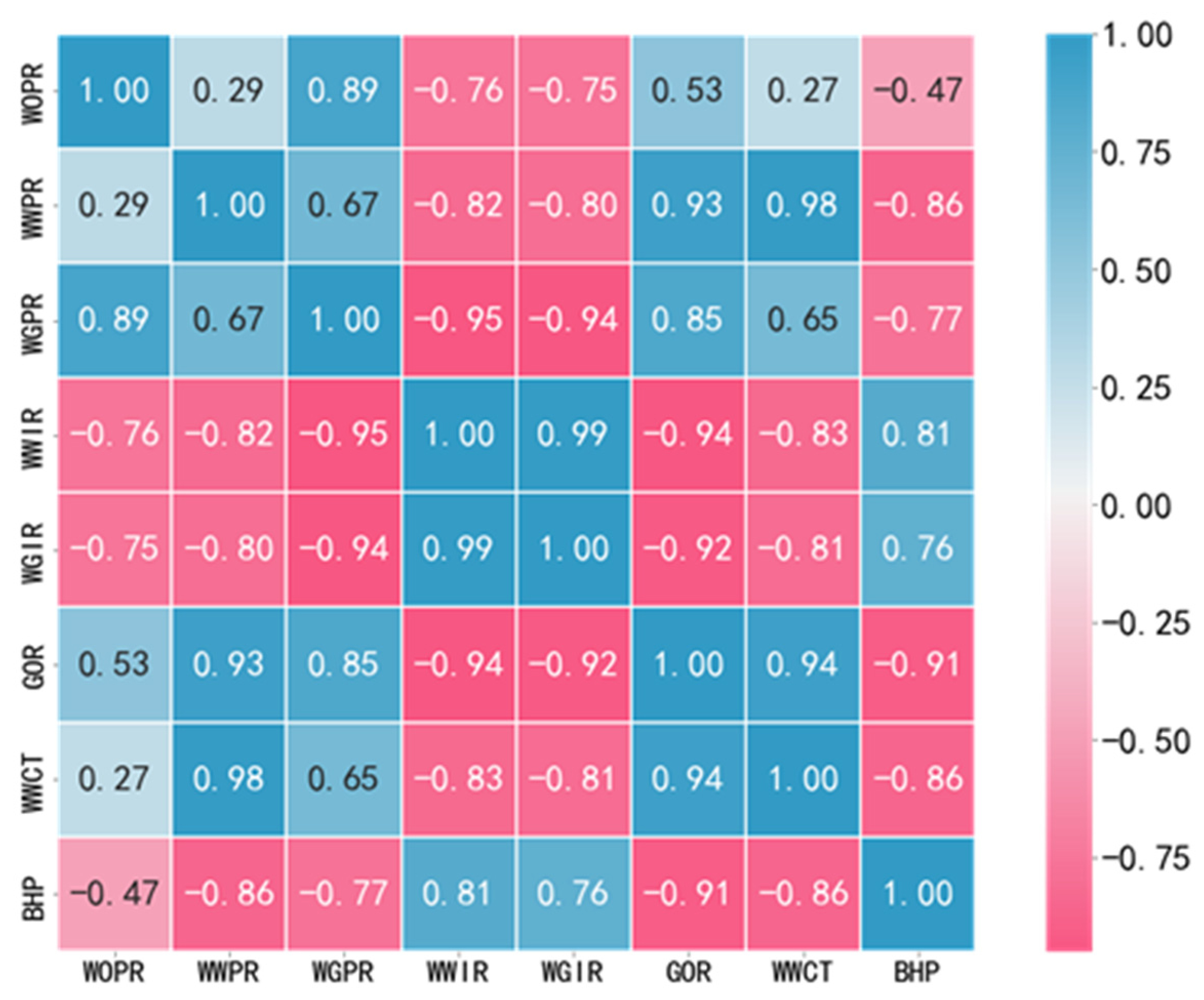
First, the Pearson algorithm [36] was employed to calculate the correlation coefficients between each pair of features, which were then represented using a heatmap as shown in Figure 3. WOPR refers to the oil production rate of a well, WWPR refers to the water production rate of a well, WGPR refers to the gas production rate of a well, WWIR refers to the water injection rate of a well, WGIR refers to the gas injection rate of a well, GOR refers to the gas–oil ratio of a well, WWCT refers to the water cut of a well, and BHP refers to the bottomhole pressure of a well. In the figure, the values of the cells where rows intersect represent the correlation between the variables represented by rows and columns. If it is a positive number, it indicates a positive correlation between these two variables, while a negative number indicates a negative correlation between these two variables. The absolute value of the correlation coefficient ranged from 0.8 to 1.0, indicating a strong correlation between features. It can be observed that variables such as the gas–oil ratio and water cut exhibited a high correlation with the bottomhole flowing pressure (−0.91 and −0.86). Additionally, there were also high correlations among the variables themselves (e.g., the correlation between WWCT and WWPR was 0.98), which could potentially interfere with the predictive performance of the model.
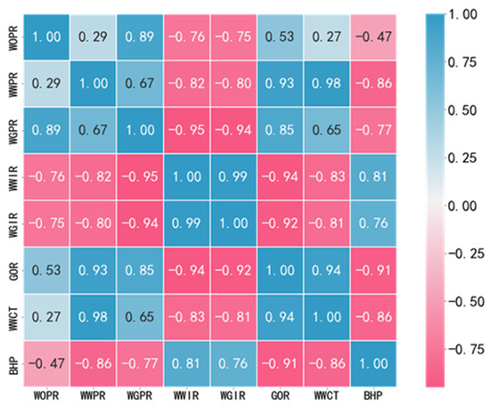
Figure 3.
Heatmap for correlation analysis of data.
A principal component analysis (PCA) [37] is a multivariate statistical algorithm used to assess the correlation between multiple variables. It employs an orthogonal transformation to convert a set of potentially correlated variables into a set of linearly uncorrelated variables called principal components. The PCA algorithm can transform the original data into several principal components while preserving as much of the original information as possible, with each principal component being mutually independent. A PCA serves the purpose of dimensionality reduction by extracting and synthesizing relevant information while reducing the interference of redundant features and accelerating the model training process.
Through the PCA algorithm, the original seven features were mapped and linearly combined to construct new features known as principal components. The importance of the principal components can be evaluated based on their contribution to the variance. A higher variance contribution indicates greater importance. We used Python to call the PCA algorithm of the scikit learn framework and reduce the data to five dimensions based on the criterion of variance contribution rate greater than 95%. The variance contribution rates of the five principal components are shown in Table 3. From Table 3, it can be observed that the first principal component contributed the most, accounting for 52.15% of the variance, while the fifth principal component contributed the least, with a variance contribution rate of 3.65%.
Table 3.
Principal component analysis data features.
The correlation heatmap of the five principal components after dimensionality reduction is presented in Figure 4. It can be seen that the absolute correlation values of the principal components after dimensionality reduction were all less than 0.5, and the principal components were independent of each other, which was conducive to the performance of the model.
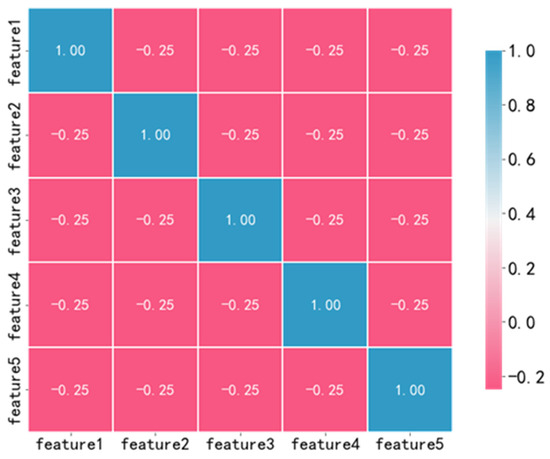
Figure 4.
Correlation analysis after dimensionality reduction.
3.3. Model Training
The corresponding parameters of the genetic algorithm used in this study are presented in Table 4. The number of generations was set to 50, as it is generally believed that if convergence is not achieved by the 50th generation, it is necessary to investigate potential issues with the data or the model, as further increasing the generations may not yield significant improvements. The population size has a certain impact on the final results, with larger populations having a higher likelihood of finding the optimal solution. However, this also increases computational complexity. To ensure a balance between accuracy and efficiency, the population size was set to 20. The significance of the convergence threshold is that if the difference between the current generation and the best values from previous generations is smaller than this threshold, it indicates that the optimization of the objective has reached a stagnation state. If the evolution stagnates beyond the maximum limit set, the algorithm will stop running.
Table 4.
The corresponding parameters of the genetic algorithm used in this paper.
The data were randomly split into training, testing, and validation sets with a 7:2:1 ratio, with the number of samples in each set presented in Table 5.
Table 5.
Number of sample sets.
Using the SEGA, the parameters were iteratively adjusted to maximize the indicator of the average adjusted R-squared score obtained through cross-validation on the training set. Cross-validation [38,39,40,41] is a practical method employed in the machine learning training process, which involves dividing the data samples into smaller subsets. By performing a K-fold cross-validation, it simulates various possible datasets, enabling a thorough testing of the model’s performance. This approach effectively utilizes the data to evaluate the model’s performance and reduces issues such as overfitting and selection bias, thereby enhancing the model’s generalization capability. Based on the empirical formula provided below, a cross-validation fold number of 6 was selected.
where represents the number of cross-validation folds and represents the size of the dataset. By randomly partitioning the data, each subset contains a mix of best- and worst-case scenarios. The cross-validated score obtained by averaging the scores from each subset may appear lower compared to the conventional training set score. However, it provides a more comprehensive evaluation of the model’s performance across different datasets, making it a suitable objective function for optimization purposes.
The R-squared coefficient of determination indicates the goodness-of-fit of the trend line. Given a series of true values () and their corresponding predicted values, R-squared is defined as follows:
The R-squared value is in the range (−∞,1] and represents the proportion of variance explained by the model. It provides an intuitive understanding of the model’s performance. As R-squared approaches 1, the model’s performance improves. But as the number of independent variables increases, the R-squared value becomes larger, and using the adjusted R-squared value to evaluate the fitting effect of the model is more accurate. The adjusted R-squared takes into account both the sample size n and the number of independent variables k. Therefore, it reflects the modelling accuracy.
RMSE (root-mean-square Error) is simultaneously used as a supplementary validation metric to assess the performance of the model. The RMSE measures the square root of the ratio between the squared deviations of the predicted values and the observed values, divided by the number of observations, n.
The RMSE quantifies the deviation between predicted values and actual values, and it is particularly sensitive to outliers in the data. A smaller RMSE value indicates higher model performance.
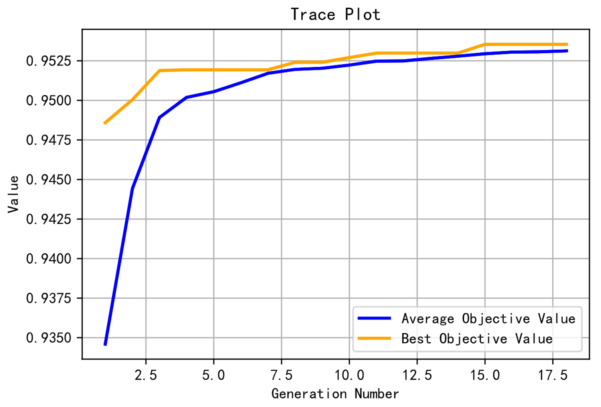
The optimization process is illustrated in Figure 5, where the average score of the population improves from below 0.9350 to above 0.9525. The final average score of the population is comparable to that of the elites. The model optimization process terminates after the 18th generation.
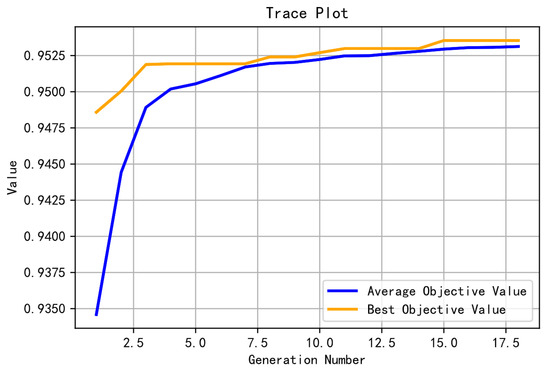
Figure 5.
Genetic algorithm optimization process.
After optimization using the genetic algorithm, the optimal values of the XGBoost parameters were found and are shown in Table 6. The average adjusted R-squared score from the cross-validation was 0.9536.
Table 6.
The parameters of the XGBoost model established in this paper.
To verify the effectiveness of XGBoost, we compared it with other common machine learning models, including support vector machines (SVM), neural networks, stochastic gradient descent (SGD), linear regression, ridge regression, decision trees, random forests, gradient boosting trees, ExtraTrees, and Adaboost. Support vector machines can handle the interaction of nonlinear features but are sensitive to missing data. Artificial neural networks can fully approximate complex nonlinear relationships but require a large number of parameters. The parameter update speed of random gradient descent is fast, but it may converge to local optima. Linear regression is easy to implement, but it cannot fit nonlinear data. Although ridge regression is less prone to overfitting compared to linear regression, it is also unable to handle nonlinear data. Decision trees are easy to understand and interpret, but they are prone to overfitting. Random forest performs well and can handle high-dimensional data, but it may overfit in some noisy problems. Gradient boosting decision trees have a good generalization ability but perform poorly on high-dimensional sparse datasets. ExtraTrees is a variant of random forests with better generalization performance at times. The Adaboost algorithm is a typical boosting algorithm that is not prone to overfitting, but imbalanced data can lead to decreased accuracy and sensitivity to outliers. Table 7 shows the parameters used by each model. These models were chosen because they have performed well in previous applications. Neural networks [13] are used for predicting bottomhole pressure in vertical multiphase flow oil wells, with a prediction error of no more than 10%. A support vector machine [42] was used for comparison in predicting bottomhole flow pressure in multiphase flow, as it represents a commonly used ML method and was therefore classified as the benchmark method in FBHP prediction. Linear regression [16] has been used to predict the bottomhole flow pressure of coalbed methane wells, with high accuracy in single-well prediction problems. Other models [43,44,45,46,47,48,49] have performed well in similar application fields.
Table 7.
The parameters used by each model.
4. Results Analysis and Comparison
4.1. Results Analysis
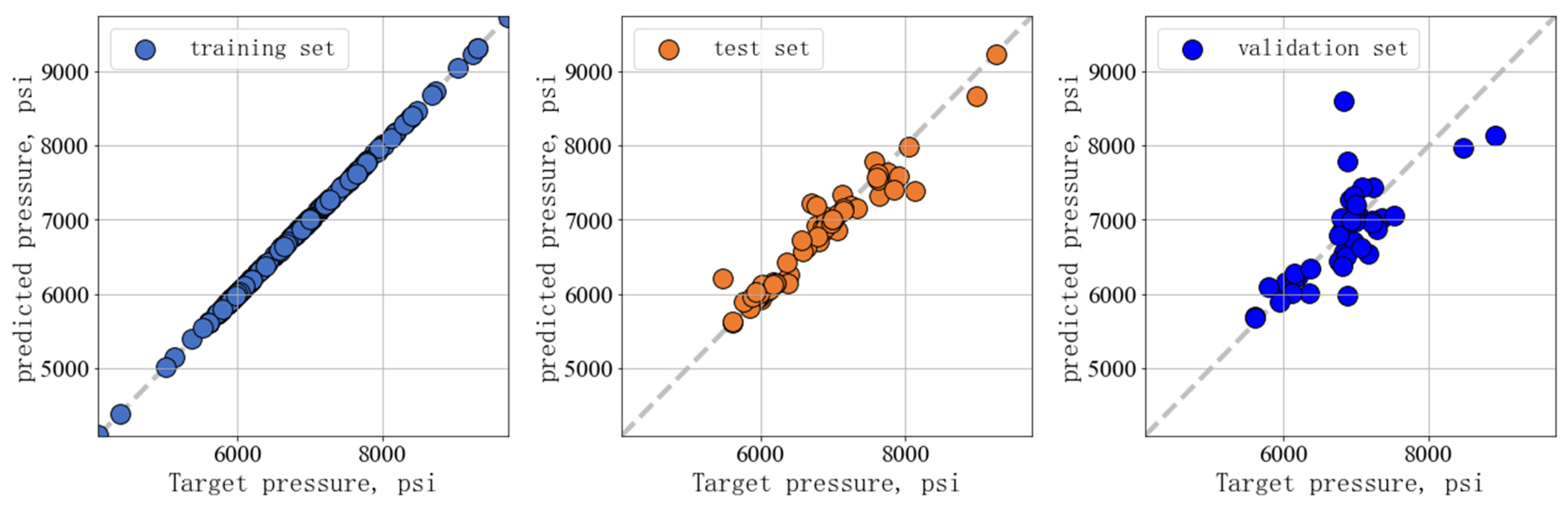
The optimized XGBoost model had an adjusted R-squared score of 0.99 and a root-mean-square error of 0.0015 on the training set; the adjusted R-squared score on the test set was 0.84, with a root-mean-square error of 0.0564; the adjusted R-squared score of the validation set was 0.68, with a root-mean-square error of 0.0721. We drew a scatter plot with the true value as X and the predicted value as Y in Figure 6, where the comparison between the true and predicted values of the model on the training, testing, and validation sets is shown. A scattered distribution above the grey dashed line indicates that the predicted value is greater than the true value, a scattered distribution below the grey dashed line indicates that the predicted value is equal to the true value, and a scattered distribution below the grey dashed line indicates that the predicted value is less than the true value. The closer the scatter points are to the grey dashed line, the closer the predicted value is to the true value. It can be seen that the points formed by the predicted values and the true values of the model in the training set are basically distributed near the line with a slope of one, indicating that the predicted values were relatively close to the true values. For unseen data, the model still performed well in both the test and validation sets, with predicted values close to actual values, indicating good generalization performance.
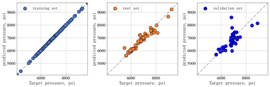
Figure 6.
Predicted versus true values of the XGBoost model.
It can be seen that the validation set has significant fluctuations in the predicted values of the model at 7000 psi, with the distribution of predicted values ranging from 6000 psi to 9000 psi, which may be due to data-driven limitations. Due to the high dependence of data-driven methods on the quality and quantity of data, the prediction error of the model for unseen data such as the validation set is relatively large compared to the training set, which is inevitable. In addition, compared with traditional models, pure data-driven models do not have physical-knowledge constraints, and some predicted values may have significant deviations. In future work, improving XGBoost by incorporating physical-knowledge constraints may lead to better predictive performance.
4.2. Comparison of Models
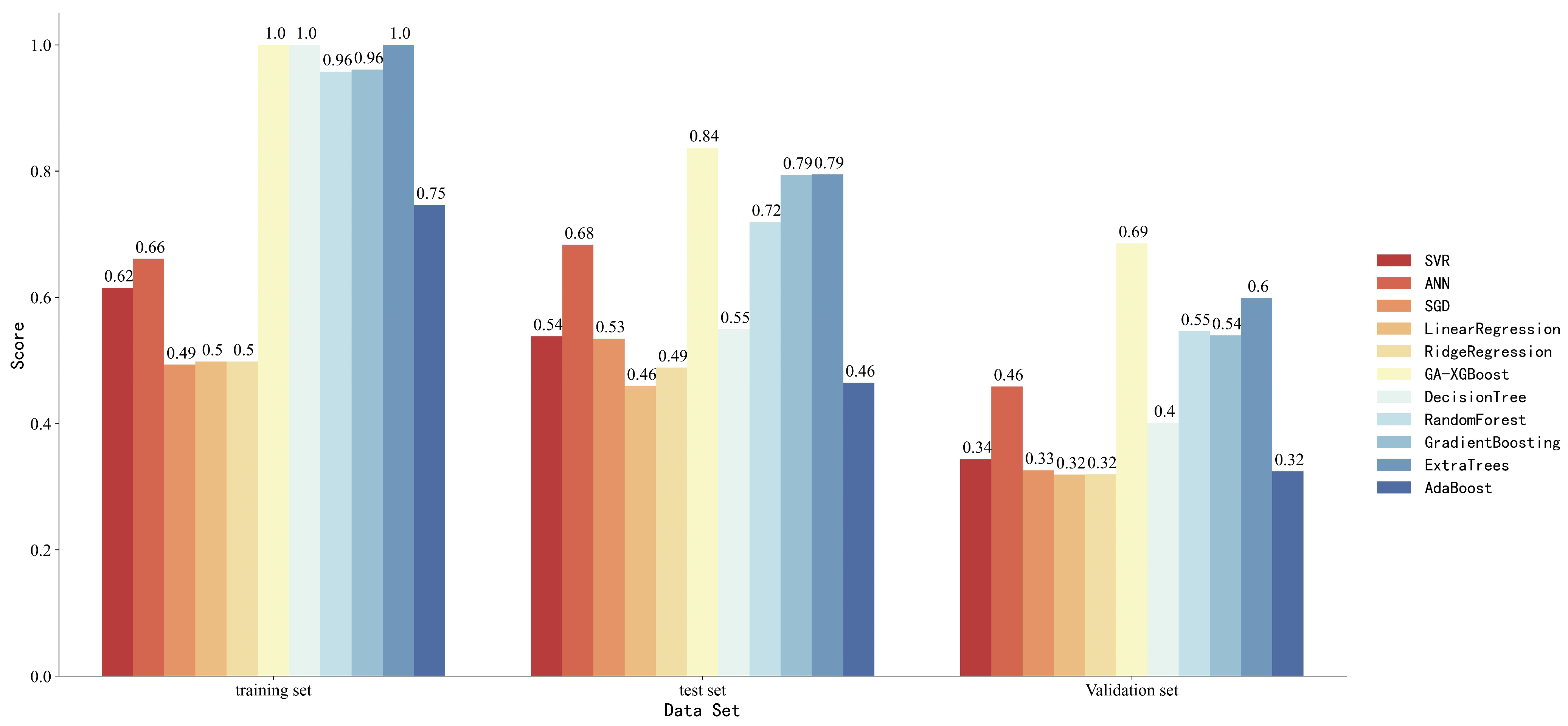
The performance of the XGBoost model was compared with that of ten other common machine learning models, including support vector machines (SVM), neural networks, stochastic gradient descent (SGD), linear regression, ridge regression, decision trees, random forests, gradient boosting trees, ExtraTrees, and Adaboost. The comparison of adjusted R-squared scores for these models on different datasets is illustrated in Figure 7.
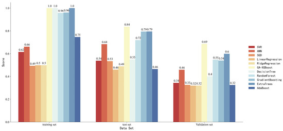
Figure 7.
Comparison of Adjusted-R-squared scores for different datasets across models.
Linear regression, ridge regression, and Adaboost models performed poorly, with scores of only 0.5, 0.51, and 0.51 on the training set. This may be due to the complex nonlinear relationship between the bottomhole pressure and input variables in heterogeneous reservoir backgrounds, and these models cannot fit nonlinear data well. Previous studies used support vector regression and neural networks for predicting bottomhole pressure, and both performed well. However, with fewer data variables, support vector regression scored only 0.62 on the training set, while the neural network scored only 0.66 on the training set. It can be observed that tree-based models, such as decision trees and random forests, exhibited superior performance compared to other machine learning algorithms like support vector machines in addressing this particular problem. The training set scores of these tree-based models consistently exceeded 0.9. However, due to their tendency to overfit, the tree-based models yielded lower scores on the testing and validation sets compared to the XGBoost model. The XGBoost model optimized by GA demonstrated excellent performance across all three datasets.
5. Discussion
In this study, we selected the XGBoost algorithm, which exhibits a high accuracy and strong generalization, to establish a bottomhole pressure prediction model for carbonate reservoirs. We used a genetic algorithm with an enhanced elite strategy to optimize XGBoost’s hyperparameters, with the objective function being the average adjusted R-squared score of a K-fold cross-validation, and compared its performance with other popular machine learning models. We selected six key variables, such as daily oil and water production, for the bottomhole pressure prediction, enabling a quick on-site implementation with limited data. The aim was to assess whether XGBoost could still perform well under limited data variable conditions. A correlation analysis revealed strong links between variables, potentially impacting the model training effectiveness. We used dimensionality reduction algorithms to convert the data into independent variables, minimizing interference from redundant features. We employed the cross-validation score as the genetic algorithm’s optimization target, enhancing data use and the model’s ability to generalize. By comparing XGBoost with commonly used machine learning algorithms, we verified the superior accuracy and generalization capabilities of XGBoost.
We established an XGBoost bottomhole pressure prediction model and optimized hyperparameters using SEGA to evaluate the pressure prediction performance of XGBoost under limited data volume. The optimized XGBoost model had an adjusted R-squared score of 0.99 and a root-mean-square error of 0.0015 on the training set; the adjusted R-squared score on the test set was 0.84, with a root-mean-square error of 0.0564; the adjusted R-squared score of the validation set was 0.69, with a root-mean-square error of 0.0721, and the superiority of GA-XGBoost was established through a comparison with other models. The poor performance of the linear regression, ridge regression, and Adaboost models may be due to the complex nonlinear relationship between the bottomhole pressure and input variables in heterogeneous reservoir backgrounds, and these models cannot fit nonlinear data well. Previous studies have used support vector regression and neural networks to predict bottomhole pressure, both of which have achieved good results. However, in the case of limited data variables, the performance of support vector regression and neural networks on the training set was also relatively average. It can be observed that tree-based models, such as decision trees and random forests, exhibited superior performance in solving this specific problem compared to other machine learning algorithms such as support vector machines. However, due to their tendency towards overfitting, tree-based models scored lower on the test and validation sets compared to XGBoost models. XGBoost, optimized by the GA model, demonstrated excellent performance on all three datasets, demonstrating the performance of the model.
6. Conclusions
The GA-XGBoost model demonstrated its ability to accurately estimate pressure values in challenging scenarios characterized by a significant heterogeneity and extreme variations in pressure distribution during the development of carbonate reservoirs. It maintained this capability even in cases with fewer data variables. This advantage of the model eliminates the need to install pressure gauges, resulting in cost savings.
Compared to numerical simulation techniques, predicting bottomhole pressure using GA-XGBoost eliminates the need for complex model building and historical fitting operations, while significantly improving computational speed. The use of genetic algorithms for automatic optimization avoids the extensive trial-and-error process required by conventional grid-search methods, saving time and effort.
Predicting the bottomhole pressure through a data-driven approach only requires commonly available production data, enabling a convenient and real-time estimation of bottomhole pressure. This method is more practical and facilitates on-site implementation of real-time bottomhole pressure prediction.
The GA-XGBoost model achieved an adjusted R-squared score of 0.99 and a root-mean-square error (RMSE) of 0.0015 on the training set. On the test set, the model obtained an adjusted R-squared score of 0.84 with an RMSE of 0.0564, while on the validation set, it achieved an adjusted R-squared score of 0.69 with an RMSE of 0.0721. Compared to other machine learning models, the GA-XGBoost model was superior in predicting bottomhole pressure with limited data features, exhibiting a high accuracy and good generalization performance. It achieved excellent results in the bottomhole pressure prediction on the training, test, and validation sets.
In future work, several trends are expected. Firstly, collecting data of various types and larger quantities will allow us to evaluate whether XGBoost’s accuracy and generalization can be improved when dealing with massive test datasets, while also assessing the computational speed of XGBoost. Secondly, introducing constraints based on prior physical knowledge during the XGBoost training process may further enhance the model’s accuracy, aligning the predicted results more closely with engineers’ understanding.
Author Contributions
Conceptualization, H.S. and Q.L.; methodology, Z.X.; software, H.S.; validation, Z.X.; formal analysis, H.S.; investigation, Q.L.; resources, Z.X.; data curation, Y.L.; writing—original draft preparation, H.S.; writing—review and editing, Y.Y.; visualization, Q.L.; supervision, Y.L. and Y.Y.; project administration, Z.X. and Y.L. All authors have read and agreed to the published version of the manuscript.
Funding
This research was funded by Major Science and Technology Special Project of the China National Petroleum Corporation, “Research on Key Technologies for Efficient Production of Overseas Large-scale Carbonate Reservoirs” (Grant No. 2023ZZ19-04).
Data Availability Statement
Data are unavailable due to privacy restrictions.
Conflicts of Interest
Author Zhaohui Xia, Yunbo Li and Yang Yu were employed by the company Research Institute of Petroleum Exploration and Development. The remaining authors declare that the research was conducted in the absence of any commercial or financial relationships that could be construed as a potential conflict of interest. All authors have read and agreed to the published version of the manuscript.
Nomenclature
| ANN | Artificial neural network |
| BHP | Bottomhole pressure of a well |
| GA | Genetic algorithm |
| GOR | Gas–oil ratio of a well |
| SGD | Stochastic gradient descent |
| SVR | Support vector regression |
| WGIR | Gas injection rate of a well |
| WGPR | Gas production rate of a well |
| WOPR | Oil production rate of a well |
| WWIR | Water injection rate of a well |
| WWCT | Water cut of a well |
| WWPR | Water production rate of a well |
| XGBoost | eXtreme Gradient Boosting |
References
- Duns, H.; Ros, N.C.J. Vertical Flow of Gas and Liquid Mixtures in Wells; OnePetro: Richardson, TX, USA, 1963. [Google Scholar]
- Hagedorn, A.R.; Brown, K.E. Experimental Study of Pressure Gradients Occurring During Continuous Two-Phase Flow in Small-Diameter Vertical Conduits. J. Pet. Technol. 1965, 17, 475–484. [Google Scholar] [CrossRef]
- Orkiszewski, J. Predicting Two-Phase Pressure Drops in Vertical Pipe. J. Pet. Technol. 1967, 19, 829–838. [Google Scholar] [CrossRef]
- Beggs, D.H.; Brill, J.P. An Experimental Study of Two-Phase Flow in Inclined Pipes. J. Pet. Technol. 1973, 25, 607–617. [Google Scholar] [CrossRef]
- Mukherjee, H.; Brill, J.P. Pressure Drop Correlations for Inclined Two-Phase Flow. J. Energy Resour. Technol. 1985, 107, 549–554. [Google Scholar] [CrossRef]
- Ansari, A.M.; Sylvester, N.D.; Sarica, C.; Shoham, O.; Brill, J.P. A Comprehensive Mechanistic Model for Upward Two-Phase Flow in Wellbores. SPE Prod. Facil. 1994, 9, 143–151. [Google Scholar] [CrossRef]
- Corsano, A. Experimental Study and the Development of a Mechanistic Model for Two-Phase Flow through Vertical Tubing. In Proceedings of the SPE Western Regional Meeting, Anchorage, AK, USA, 22–24 May 1996; SPE: Kuala Lumpur, Malaysia, 1996. [Google Scholar]
- Gomez, L.E.; Shoham, O.; Schmidt, Z.; Chokshi, R.N.; Northug, T. Unified Mechanistic Model for Steady-State Two-Phase Flow: Horizontal to Vertical Upward Flow. SPE J. 2000, 5, 339–350. [Google Scholar] [CrossRef]
- Wang, B. The Latest Application of Artificial Intelligence Technology in Petroleum Engineering Field. China CIO News 2018, 10, 95. [Google Scholar]
- Zhao, X.; Chen, X.; Lan, Z.; Wang, X.; Yao, G. Pore Pressure Prediction Assisted by Machine Learning Models Combined with Interpretations: A Case Study of an HTHP Gas Field, Yinggehai Basin. Geoenergy Sci. Eng. 2023, 229, 212114. [Google Scholar] [CrossRef]
- Awadalla, M.; Yousef, H. Neural Networks for Flow Bottom Hole Pressure Prediction. Int. J. Electr. Comput. Eng. IJECE 2016, 6, 1839. [Google Scholar] [CrossRef]
- Firouzi, M.; Rathnayake, S. Prediction of the Flowing Bottom-Hole Pressure Using Advanced Data Analytics; OnePetro: Richardson, TX, USA, 2019. [Google Scholar]
- Ahmadi, M.A.; Chen, Z. Machine Learning Models to Predict Bottom Hole Pressure in Multi-phase Flow in Vertical Oil Production Wells. Can. J. Chem. Eng. 2019, 97, 2928–2940. [Google Scholar] [CrossRef]
- Nait Amar, M.; Zeraibi, N.; Redouane, K. Bottom Hole Pressure Estimation Using Hybridization Neural Networks and Grey Wolves Optimization. Petroleum 2018, 4, 419–429. [Google Scholar] [CrossRef]
- Nait Amar, M.; Zeraibi, N. A Combined Support Vector Regression with Firefly Algorithm for Prediction of Bottom Hole Pressure. SN Appl. Sci. 2020, 2, 23. [Google Scholar] [CrossRef]
- Rathnayake, S.; Rajora, A.; Firouzi, M. A Machine Learning-Based Predictive Model for Real-Time Monitoring of Flowing Bottom-Hole Pressure of Gas Wells. Fuel 2022, 317, 123524. [Google Scholar] [CrossRef]
- Jia, D.; Liu, H.; Zhang, J.; Pei, X.; Wang, Q.; Yang, Q. Data-Driven Optimization for Fine Water Injection in a Mature Oil Field. Pet. Explor. Dev. 2020, 47, 629–636. [Google Scholar] [CrossRef]
- Wang, H.; Mu, L.; Shi, F.; Dou, H. Production Prediction at Ultra-High Water Cut Stage via Recurrent Neural Network. Pet. Explor. Dev. 2020, 47, 1009–1015. [Google Scholar] [CrossRef]
- Tariq, Z.; Mahmoud, M.; Abdulraheem, A. An Artificial Intelligence Approach to Predict the Water Saturation in Carbonate Reservoir Rocks; OnePetro: Richardson, TX, USA, 2019. [Google Scholar]
- Artun, E.; Kulga, B. Selection of Candidate Wells for Re-Fracturing in Tight Gas Sand Reservoirs Using Fuzzy Inference. Pet. Explor. Dev. 2020, 47, 383–389. [Google Scholar] [CrossRef]
- Chen, T.; Guestrin, C. XGBoost: A Scalable Tree Boosting System. In Proceedings of the 22nd ACM SIGKDD International Conference on Knowledge Discovery and Data Mining, San Francisco, CA, USA, 13 August 2016; pp. 785–794. [Google Scholar]
- Ogunleye, A.; Wang, Q.-G. XGBoost Model for Chronic Kidney Disease Diagnosis. IEEE/ACM Trans. Comput. Biol. Bioinform. 2020, 17, 2131–2140. [Google Scholar] [CrossRef]
- Dhaliwal, S.S.; Nahid, A.-A.; Abbas, R. Effective Intrusion Detection System Using XGBoost. Information 2018, 9, 149. [Google Scholar] [CrossRef]
- Pan, S.; Zheng, Z.; Guo, Z.; Luo, H. An Optimized XGBoost Method for Predicting Reservoir Porosity Using Petrophysical Logs. J. Pet. Sci. Eng. 2022, 208, 109520. [Google Scholar] [CrossRef]
- Markovic, S.; Bryan, J.L.; Rezaee, R.; Turakhanov, A.; Cheremisin, A.; Kantzas, A.; Koroteev, D. Application of XGBoost Model for In-Situ Water Saturation Determination in Canadian Oil-Sands by LF-NMR and Density Data. Sci. Rep. 2022, 12, 13984. [Google Scholar] [CrossRef] [PubMed]
- Zhong, R.; Johnson, R.; Chen, Z. Generating Pseudo Density Log from Drilling and Logging-While-Drilling Data Using Extreme Gradient Boosting (XGBoost). Int. J. Coal Geol. 2020, 220, 103416. [Google Scholar] [CrossRef]
- Gu, Y.; Zhang, D.; Bao, Z. A New Data-Driven Predictor, PSO-XGBoost, Used for Permeability of Tight Sandstone Reservoirs: A Case Study of Member of Chang 4+5, Western Jiyuan Oilfield, Ordos Basin. J. Pet. Sci. Eng. 2021, 199, 108350. [Google Scholar] [CrossRef]
- Al-Mudhafar, W.J.; Abbas, M.A.; Wood, D.A. Performance Evaluation of Boosting Machine Learning Algorithms for Lithofacies Classification in Heterogeneous Carbonate Reservoirs. Mar. Pet. Geol. 2022, 145, 105886. [Google Scholar] [CrossRef]
- Zhang, J.; Sun, Y.; Shang, L.; Feng, Q.; Gong, L.; Wu, K. A Unified Intelligent Model for Estimating the (Gas + n-Alkane) Interfacial Tension Based on the eXtreme Gradient Boosting (XGBoost) Trees. Fuel 2020, 282, 118783. [Google Scholar] [CrossRef]
- Dong, Y.; Qiu, L.; Lu, C.; Song, L.; Ding, Z.; Yu, Y.; Chen, G. A Data-Driven Model for Predicting Initial Productivity of Offshore Directional Well Based on the Physical Constrained eXtreme Gradient Boosting (XGBoost) Trees. J. Pet. Sci. Eng. 2022, 211, 110176. [Google Scholar] [CrossRef]
- Wang, Z.; Tang, H.; Cai, H.; Hou, Y.; Shi, H.; Li, J.; Yang, T.; Feng, Y. Production Prediction and Main Controlling Factors in a Highly Heterogeneous Sandstone Reservoir: Analysis on the Basis of Machine Learning. Energy Sci. Eng. 2022, 10, 4674–4693. [Google Scholar] [CrossRef]
- Zhai, L. XGBoost-Based Water Injection Profile Prediction Method and Its Application. Pet. Geol. Recovery Effic. 2022, 29, 175–180. [Google Scholar] [CrossRef]
- Shi, J.; Xu, H.; Peng, L. Research on Complaint Management System of Manufacturing Industry Based on XGBoost. Manuf. Autom. 2023, 45, 76–79. [Google Scholar]
- Chen, K.-Y. Forecasting Systems Reliability Based on Support Vector Regression with Genetic Algorithms. Reliab. Eng. Syst. Saf. 2007, 92, 423–432. [Google Scholar] [CrossRef]
- Whitley, D. A Genetic Algorithm Tutorial. Stat. Comput. 1994, 4, 65–85. [Google Scholar] [CrossRef]
- Benesty, J.; Chen, J.; Huang, Y.; Cohen, I. Pearson Correlation Coefficient. In Noise Reduction in Speech Processing; Cohen, I., Huang, Y., Chen, J., Benesty, J., Eds.; Springer Topics in Signal Processing; Springer: Berlin/Heidelberg, Germany, 2009; pp. 1–4. ISBN 978-3-642-00296-0. [Google Scholar]
- Wold, S.; Esbensen, K.; Geladi, P. Principal Component Analysis. Chemom. Intell. Lab. Syst. 1987, 2, 37–52. [Google Scholar] [CrossRef]
- Rahimi, M.; Riahi, M.A. Reservoir Facies Classification Based on Random Forest and Geostatistics Methods in an Offshore Oilfield. J. Appl. Geophys. 2022, 201, 104640. [Google Scholar] [CrossRef]
- Wang, G.; Ju, Y.; Carr, T.R.; Li, C.; Cheng, G. Application of Artificial Intelligence on Black Shale Lithofacies Prediction in Marcellus Shale, Appalachian Basin; OnePetro: Richardson, TX, USA, 2014. [Google Scholar]
- Al-Mudhafar, W.J. Incorporation of Bootstrapping and Cross-Validation for Efficient Multivariate Facies and Petrophysical Modeling; OnePetro: Richardson, TX, USA, 2016. [Google Scholar]
- Pirrone, M.; Battigelli, A.; Ruvo, L. Lithofacies Classification of Thin Layered Reservoirs through the Integration of Core Data and Dielectric Dispersion Log Measurements; OnePetro: Richardson, TX, USA, 2014. [Google Scholar]
- Marfo, S.A.; Asante-Okyere, S.; Ziggah, Y.Y. A new flowing bottom hole pressure prediction model using M5 prime decision tree approach. Model. Earth Syst. Environ. 2022, 8, 2065–2073. [Google Scholar] [CrossRef]
- Sun, P.; Huo, S.; He, T. Multiple machine learning models in estimating viscosity of crude oil: Comparisons and optimization for reservoir simulation. J. Mol. Liq. 2023, 384, 122251. [Google Scholar] [CrossRef]
- Fan, P.; Deng, R.; Qiu, J.; Zhao, Z.; Wu, S. Well logging curve reconstruction based on kernel ridge regression. Arab. J. Geosci. 2021, 14, 1559. [Google Scholar] [CrossRef]
- Üneş, F.; Demirci, M.; Taşar, B.; Kaya, Y.Z.; Varçin, H. Modeling of dam reservoir volume using generalized regression neural network, support vector machines and M5 decision tree models. Appl. Ecol. Environ. Res. 2019, 17, 7043–7055. [Google Scholar] [CrossRef]
- Wang, M.; Feng, D.; Li, D.; Wang, J. Reservoir Parameter Prediction Based on the Neural Random Forest Model. Front. Earth Sci. 2022, 10, 888933. [Google Scholar] [CrossRef]
- Qin, Y.; Ye, Z.; Zhang, C. Application of GBDT for division of petroleum reservoirs. J. Phys. Conf. Ser. 2020, 1437, 012050. [Google Scholar] [CrossRef]
- Seyyedattar, M.; Zendehboudi, S.; Butt, S. Relative permeability modeling using extra trees, ANFIS, and hybrid LSSVM–CSA methods. Nat. Resour. Res. 2022, 31, 571–600. [Google Scholar] [CrossRef]
- Busari, G.A.; Lim, D.H. Crude oil price prediction: A comparison between AdaBoost-LSTM and AdaBoost-GRU for improving forecasting performance. Comput. Chem. Eng. 2021, 155, 107513. [Google Scholar] [CrossRef]

Disclaimer/Publisher’s Note: The statements, opinions and data contained in all publications are solely those of the individual author(s) and contributor(s) and not of MDPI and/or the editor(s). MDPI and/or the editor(s) disclaim responsibility for any injury to people or property resulting from any ideas, methods, instructions or products referred to in the content. |
© 2024 by the authors. Licensee MDPI, Basel, Switzerland. This article is an open access article distributed under the terms and conditions of the Creative Commons Attribution (CC BY) license (https://creativecommons.org/licenses/by/4.0/).