Oil Production Optimization Using Q-Learning Approach

Abstract

This paper presents an approach for optimizing the oil recovery factor by determining initial oil production rates. The proposed method utilizes the Q-learning method and the reservoir simulator (Eclipse 100) to achieve the desired objective. The system identifies the most efficient initial oil production rates by conducting a sufficient number of iterations for various initial oil production rates. To validate the effectiveness of the proposed approach, a case study is conducted using a numerical reservoir model (SPE9) with simplified configurations of two producer wells and one injection well. The simulation results highlight the capabilities of the Q-learning method in assisting reservoir engineers by enhancing the recommended initial rates.

1. Introduction

In spite of efforts to promote the widespread adoption of cleaner energy sources, such as renewables, the reliance on fossil fuels is expected to persist for several decades to come. Projections indicate that global energy demand is set to rise by 37% by 2040, with over half of the energy consumers continuing to rely on fossil fuel-derived sources. While the COVID-19 pandemic has had a slight impact on energy demand, the oil and gas industry is expected to gradually recover and resume its original pace, expanding its exploration and production activities to meet the increasing needs of consumers [1].

The increase in global oil prices has incentivized producers to adopt new technological advancements. Enhanced oil recovery (EOR) encompasses a range of advanced techniques aimed at maximizing oil extraction from reservoirs [2]. Maximizing oil recovery from mature reservoirs is crucial for both environmental impact and economic purposes, and a variety of strategies are available for this purpose. However, the industry still needs to develop innovative techniques and technologies to optimize oil production and increase oil recovery from mature reservoirs.

Several studies with various approaches have worked on optimizing oil production operations to improve the oil recovery rate while minimizing the operating cost and injection gas rate. The methods used, including derivative-free optimization methods, genetic algorithms, and global optimization techniques, all showed improved optimization performance and efficiency of the production and injection processes. The proposed methods and approaches provide cost-effective ways to improve the performance of waterflooding, well management strategy, and gas-lift allocation process.

Echeverria Ciaurri et al. [3] conducted an examination of derivative-free techniques applied to optimize oil production in the presence of general constraints. The considered techniques include generalized pattern search, Hooke-Jeeves direct search, genetic algorithms, and gradient-based algorithms employing numerical estimation of derivatives. The findings demonstrate the favorable performance of derivative-free algorithms, particularly when used within a distributed computing framework, leading to significant improvements in efficiency.

Martinez et al. [4] focused on applying a genetic algorithm (GA) to enhance the production optimization process in gas lift-operated oil fields. This computational methodology has proven highly effective and efficient in achieving the desired objective. The GA enables production engineers to determine suitable gas injection rates for individual wells while considering the total gas supply available in the field. By ensuring compatibility with the available gas supply and maximizing overall liquid production, this approach yields favorable results.

Buitrago et al. [5] addressed the limitations of the conventional equal slope allocation method. They proposed an automated methodology to determine the optimal gas injection rate for a group of wells, aiming to maximize overall oil production while adhering to specific constraints on the available gas volume. Their proposed approach combines stochastic domain exploration with heuristic calculations to prevent the algorithm from being trapped in local optima.

Wang et al. [6] introduced a new problem formulation for flow interactions among wells, accommodating different levels of complexity. They solved the optimization problem utilizing a sequential quadratic programming algorithm and found that this approach effectively manages intricate oil production challenges.

Fang and Lo [7] introduced an innovative approach to well management, aiming to maximize oil production while considering multiple constraints within the production facilities. Their proposed scheme integrates various factors, including reservoir performance, wellbore hydraulics, surface facility limitations, and lift-gas allocation, to optimize oil production. By utilizing up-to-date information on hydraulics and reservoir conditions, the scheme provides accurate predictions of well performance. Its effectiveness was demonstrated through implementation in a black oil simulator using separable programming and the simplex algorithm, resulting in efficient production optimization. The scheme was applied to two full-field models, where oil production is restricted by constraints such as water, gas, and liquid handling limitations at both field and flow-station levels, as well as gas injectivity and gas handling limits. Over a 12-year production forecast, the scheme successfully increased oil production by 3% to 9%.

Albertoni and Lake [8] presented a practical methodology for quantifying communication between wells in a reservoir using production and injection rate data. The approach combines constrained multivariate linear regression analysis and diffusivity filters to extract valuable insights into permeability trends and the presence of transmissibility barriers. The methodology was developed, validated using a numerical simulator, and subsequently applied to a waterflooded field in Argentina. The simulation results demonstrated that the connectivity between wells could be characterized by coefficients determined solely by the geological characteristics and relative positions of the wells, independent of injection or production rates. These findings have important implications for improving the performance of existing waterflood operations by suggesting potential modifications to well patterns and management strategies. Furthermore, the results can be utilized for reservoir flow modeling purposes.

Dutta-Roy and Kattapuram [9] focused on overcoming the limitations of existing methods for determining the optimal gas-lift injection rate in wells. These methods often overlook practical complexities and the interactions between wells in the gathering network, leading to overly optimistic results. Another challenge arises from the limited capacity of available compressors, which may not meet the increasing gas requirements as the field depletes. To address these issues, they propose a novel approach that combines a rigorous pressure-balance-based multiphase flow network solving technique with a robust sequential quadratic programming (SQP) approach for constrained optimization. The effectiveness of the proposed technique is evaluated by applying it to field-wide problems and comparing the results with conventional analysis methods. The paper also emphasizes the impact of various factors, including reservoir depletion behavior, varying water-cut, capital and operating costs, and compressor performance, on the economics of implementing a field-wide gas-lift strategy.

Some studies have focused on the application of reinforcement learning (RL) techniques for optimizing oil and gas production.

De Paola et al. [10] focused on determining the optimal drilling decision in a Field Development Plan (FDP) by employing a sequential approach using Dynamic Programming (DP) and Reinforcement Learning (RL). The FDP optimization problem is modeled as a Partially Observable Markov Decision Process (POMDP), and RL algorithms are used to find the best drilling policy. A Deep Recurrent Neural Network (RNN) is trained to approximate reservoir simulator flows, enabling the calculation of economic performance based on discounted cash flows. The RL agent improves the drilling schedule policy iteratively by utilizing a neural network trained across episodes. The methodology is applied to a real reservoir for infill well location decisions, leading to the identification of the optimal drilling plan. The solution’s robustness is assessed, and the methodology is validated using a brute-force sampling approach. This research represents the first application of an end-to-end AI workflow for Field Development Policy Evaluation, employing Reinforcement Learning and Deep Learning techniques, and demonstrates the effectiveness of the proposed methodology in field evaluation and decision-making processes.

Miftakhov et al. [11] presented an application of Deep Reinforcement Learning (RL) to maximize the Net Present Value (NPV) of waterflooding by adjusting the water injection rate. By utilizing pixel information, the study highlights the benefits of RL in enhancing reservoir physics understanding without explicitly considering reservoir properties and well parameters. The RL-based optimization routine is implemented on a 2D model that represents a vertical section of the SPE 10 model, demonstrating its effectiveness in optimizing water flooding in a 2D compressible reservoir with oil-water two-phase flow. The optimization process is iterative, initially resulting in a similar NPV to the baseline due to the convergence time needed for raw pixel data. However, RL optimization ultimately improves the NPV by 15%, leading to a more favorable scenario with reduced water-cut values and increased production stability. The results reveal that RL optimization exploits the limitations of the reservoir simulation engine, imitating a cyclic injection regime and achieving a 7% higher NPV compared to the alternative case.

Ma et al. [12] investigated the utilization of four advanced deep reinforcement learning (RL) algorithms, namely deep Q-network (DQN), double DQN (DDQN), dueling DDQN, and deep deterministic policy gradient (DDPG), to optimize the net present value (NPV) of waterflooding (WF) by adjusting the water injection rate while considering geological uncertainties. A collection of fifty reservoir models is generated using geostatistical techniques to account for these uncertainties. The findings demonstrate the effectiveness of these deep RL algorithms in optimizing WF in a 3-D 3-phase reservoir (oil–water–gas) under geological uncertainties. Notably, DQN and particle swarm optimization (PSO) converge to the same highest NPV, while the other three deep RL algorithms may converge to local optimum NPVs due to challenges related to exploration-exploitation. DDPG exhibits faster convergence compared to PSO and requires fewer numerical simulation runs. Moreover, optimizing the water injection rate, while considering geological uncertainties, leads to increased expected NPV and reduced standard deviation. The study also identifies the optimal starting time for WF during the primary production phase, which ensures continued solution-gas drive and mitigates water-cut. A comparative analysis of production performance is conducted for three different water injection scenarios: no-control, reactive-control, and optimum-control. The the optimum-control scenario demonstrates a favorable outcome with a low water-cut and stable oil production.

Zhang et al. [13] introduced a novel method for optimizing the net present value (NPV) throughout the life-cycle of production and enabling real-time adjustments to the well control scheme. The approach formulates the optimization problem as a finite-horizon Markov decision process (MDP), treating the well-control scheme as a sequence of decisions. By employing the soft actor-critic algorithm, a model-free deep reinforcement learning (DRL) technique, the study trains a DRL agent to maximize long-term NPV rewards and control scheme randomness. The agent learns a stochastic policy mapping reservoir states to well control variables and an action-value function estimating the current policy’s objective value. This trained policy enables the DRL agent to dynamically adapt the well control scheme in response to reservoir conditions. Unlike other approaches relying on sensitive parameters or complex structures, the DRL agent learns adaptively by interacting with uncertain reservoir environments and leveraging accumulated well control experience. This methodology closely resembles actual field well control practices and utilizes gradient information for improved sample efficiency. Simulation results on two reservoir models demonstrate the superiority of the proposed method over alternative optimization approaches, achieving higher NPV and demonstrating excellent performance in terms of oil displacement.

Talavera et al. [14] introduced a new methodology that combines Model Predictive Control (MPC) with machine learning techniques, specifically Reinforcement Learning (RL) and neural networks, to optimize control policies and simulate nonlinear oil reservoir systems. A neural network model is developed to predict various variables, including average reservoir pressure, daily production of oil, gas, water, and water-cut in the production well, for three consecutive time steps. These predictions are then used as inputs for the predictive control. The methodology is applied to regulate oil production in a synthetic reservoir model with layered permeability, featuring a producer well and an injector well completed in all layers. The control variables are the valves in the injector well, while the oil production of the producer well is the controlled variable. Experimental findings demonstrate the efficacy of the proposed model in maintaining control over oil production, even when faced with disturbances and varying reference values. The model effectively addresses the challenges posed by nonlinearity, system response delay, and multivariate characteristics commonly encountered in petroleum reservoir systems.

Our research introduces a novel tool that, in conjunction with existing reservoir engineering tools, assists in determining the optimal initial production and injection well rates for maximizing the oil recovery factor. The proposed method takes a higher-level approach, avoiding the intricacies of complex details, and employs Q-learning as an artificial intelligence technique. By collaborating with the reservoir simulator, the reinforcement learning method evaluates the value of each chosen action and propels the rate selection process towards the optimal trajectory. Initially, the reservoir engineer provides the initial rates, which are then synchronized with a reservoir simulator (ECLIPSE 100). Subsequently, the method iteratively adjusts the rates, aiming to optimize the oil recovery factor.

The realm of oil and gas is inherently complex, encompassing a multitude of factors. Considering all these factors simultaneously adds computational intricacy to studies in this domain. In these investigations, simplification becomes a necessity. On the other hand, the Q-Learning method represents a model-free reinforcement learning technique, capable of learning the environment without the need for train data. Therefore, when employing this approach, there is no obligation to consider each factor individually or wait for extensive data over extended periods. Unlike other supervised learning methods reliant solely on previous data, Q-Learning is a technique that can adapt and learn from the current available data, factors, and conditions, whether complete or partial. For these reasons, opting for the Q-Learning method for research in the oil sector is entirely rational and fitting. These explanations will be utilized to enhance the comprehensiveness of the introduction.

The remainder of the paper is structured as follows: In Section 2, titled “Q-Learning Method in Oil Production Optimization”, we provide a detailed explanation of how an oil well reservoir is modeled in this study and how the Q-Learning algorithm can be effectively employed in the context of oil production optimization. Section 3, “Evaluation of the Method”, focuses on the evaluation and analysis of the proposed approach. We describe the experimental setup and data collection process and present the results obtained from applying the Q-Learning method to a real-world oil production system. Through comprehensive performance metrics and comparative analysis, we assess the effectiveness and efficiency of the Q-Learning method in optimizing oil production processes. Finally, in Section 4, “Conclusions”, we summarize the main findings and contributions of this study. We highlight the advantages and limitations of the Q-Learning approach and discuss potential areas for future research and improvements. The conclusions drawn from our investigation provide valuable insights for the oil industry, demonstrating the potential of Q-Learning as a viable solution for enhancing oil production optimization strategies.

2. Q-Learning Method in Oil Production Optimization

Oil wells are drilled into the ground to extract crude oil and its accompanying natural gas. The gas obtained from these wells is commonly treated in order to generate natural gas liquids [15]. Over the past few years, oil production companies and environmental agencies have shown increasing interest in enhancing reservoir production optimization. The objective is to maximize revenue generated from oil and gas extraction while simultaneously reducing operating expenses. Optimization algorithms play a crucial role in identifying favorable or optimal outcomes, offering a systematic approach to achieving this objective [16].

The oil recovery factor serves as a metric for quantifying oil production and can be understood as the proportion of extracted oil relative to the total amount of oil in the reservoir. Equation (1) provides the mathematical expression used to compute the oil recovery factor.

$$FOE=\frac{OIP\left(initial\right)-OIP\left(now\right)}{OIP\left(initial\right)}.$$

(1)

In Equation (1), FOE stands for Field Oil recovery Efficiency. In reservoir simulator (ECLIPSE), it is called oil recovery factor. OIP (initial) stands for initial oil in the reservoir, and OIP (now) stands for the current amount of oil in the reservoir. By considering the rate of $wel{l}_i$ as $r_i$, the goal of the developed system is to establish a set of initial rates (R) so that the oil recovery factor will be optimized. Based on the well’s limitations, reservoir engineers choose a range of values for $r_i$ that satisfy these limitations.

The choice of Eclipse is solely based on the authors’ permission to use it, and any other simulator could be substituted in its place. This method is independent of simulator choice and is capable of encompassing various complex data and factors. It has the capability to re-derive all the results of the paper regardless of the selected simulator. In fact, any output obtained from these simulators can be utilized as data in our method, and the simulator itself is not the focus of the article’s subject matter.

The Q-learning method falls under the category of Reinforcement Learning, which draws inspiration from various natural behaviors. This algorithm learns about the environment through a trial-and-error approach. Rewards, either negative or positive, are assigned for incorrect or correct actions, respectively. By remembering past actions and aiming to accumulate the highest rewards, the system strives to perform actions correctly or choose the optimal values [17,18].

A significant challenge in using Q-learning is finding the right balance between exploration and exploitation. This balance is crucial for the agent to effectively learn and understand the environment [19]. In our case, the motivation for utilizing Q-learning stems from the nature of oil reservoirs. The interconnectedness of all the wells necessitates integrated production optimization for all wells simultaneously. Additionally, the oil reservoir environment exhibits a high level of uncertainty due to numerous dynamics and variables, often exhibiting nonlinear relationships. Assuming parameter independence may lead to overlooking critical aspects of the problem. By employing the Q-learning algorithm as a model-free approach, we can navigate the goal through trial and error, regardless of the number, dependence, and complexity of the parameters.

2.1. Modelling an Oil Well Reservoir

The production of wells within an oil reservoir is interconnected, meaning that optimizing the production of individual wells does not lead to overall reservoir production optimization. Therefore, there is a need for a model that takes an integrated approach to view and optimize the production of all wells.

Figure 1 illustrates the system’s perspective on an oil reservoir, considering it as a directed acyclic graph. Each node in the graph represents an oil well with a single possible rate value, denoted as $wel{l}_n-rat{e}_m$. The objective is to select an appropriate set of well rates to optimize the recovery factor.

The proposed model achieves this goal through an iterative process. Each episode begins by selecting well rates starting from the initial node, followed by choosing well rates suggested by the Q-learning (QL) algorithm, and concluding with the selection of the proper rate for the last well ($wel{l}_n-rat{e}_m$). The chosen well rates serve as inputs for the simulator, which is treated as a black box in this model. The QL algorithm’s new suggestion for the well-rate set initiates the next episode. One advantage of this approach is its independence from the initial point and its ability to avoid being trapped in local minima. The data serve as input for the Q-learning method, and they can even be incomplete. The learning process takes place based on the available data, and the data can gradually be completed over time.

2.2. Implementing the Q-Learning Technique

According to Figure 1, there are multiple choices that the system can make in one episode, specifically $wellnumber\times ratenumber$ possibilities. Testing all these options is a viable approach to selecting an optimal well-rate set, but it would be time-consuming. Therefore, an algorithm that can provide an acceptable rate list within a reasonable runtime is needed. A reinforcement learning algorithm is a suitable option as it gradually approaches the solution. The longer it runs, the better results it can achieve.

Furthermore, due to the vast and uncertain nature of the petroleum industry, it is nearly impossible to have complete knowledge of all interrelated parameters. In this context, Q-learning serves as a promising candidate. It is a model-free approach that discovers the goal through a process of trial and error, making it well-suited for addressing the challenges of uncertainty in the petroleum industry.

In order to implement the Q-learning algorithm, it is necessary to define its parameters as follows:

• Each node depicted in Figure 1 is treated as an individual state within the algorithm.
• The selection of the next state, which guides the system from one state ($stat{e}_s$) to another ($stat{e}_s^{\prime }$), is regarded as an action.
• Once the system has traversed all the wells, one complete episode is considered to be finished.
• The Q-table is used as the system’s memory. Initially, it is initialized with zero values since the system lacks knowledge about the environment.
• The reward table, which stores the rewards associated with each state-action pair, is referred to as the reward table.
• The action selection method utilized in this system is called $ϵ-greedy$. This method ensures that, after a sufficient number of iterations, the optimal policy will be determined. $ϵ$ plays a significant role in balancing the system’s exploration and exploitation. Initially, $ϵ$ is set to 0.3, which means that in 30% of the actions, the system explores new areas. As the iterations progress, $ϵ$ is gradually reduced to zero. The values set for epsilon and alpha are the result of validation, as commonly used in machine learning methods. With these settings, the system exhibits effective training and converges well.

$$Q(s,a)=Q(s,a)+\alpha [r+\gamma Ma{x}_{a^{\prime }}Q(s^{\prime },a^{\prime })-Q(s,a)].$$

(2)

Equation (2) presents the QL algorithm updates. It is based on the feedback received from the simulator regarding the previous episode’s well-rates. The procedure repeats itself continually until the algorithm converges to an optimized oil recovery factor. In Equation (2), $Q(s,a)$ presents the Q-table for state s and action a. The system observes the current state s and chooses an action a. It observes the reward r and transfers to the new state $s^{\prime }$. $maxQ(s^{\prime },a^{\prime })$ presents the updated Q-table using the maximum possible reward for state $s^{\prime }$ and action $a^{\prime }$. $\alpha$ is the learning rate, which is initiated by 0.5. By this choice we let the system use 0.5 of its recent experiences and learn from 0.5 of future results. Then after some iterations it is decreased to zero.

Equation (2) describes the update process of the Q-learning (QL) algorithm. It relies on the feedback provided by the simulator regarding the well-rates used in the previous episode. This procedure repeats continuously until the algorithm reaches an optimized oil recovery factor. In Equation (2), $Q(s,a)$ represents the Q-table entry for a given state s and action a. The system observes the current state s and selects an action a. It then observes the reward r and transitions to a new state $s^{\prime }$. The term $maxQ(s^{\prime },a^{\prime }$) represents the updated Q-table value, using the maximum possible reward for the state $s^{\prime }$ and action $a^{\prime }$. The learning rate $\alpha$, initially set to 0.5, determines how much the system utilizes its recent experiences (0.5) and learns from future outcomes (0.5). After several iterations, the learning rate is decreased gradually, eventually reaching zero.

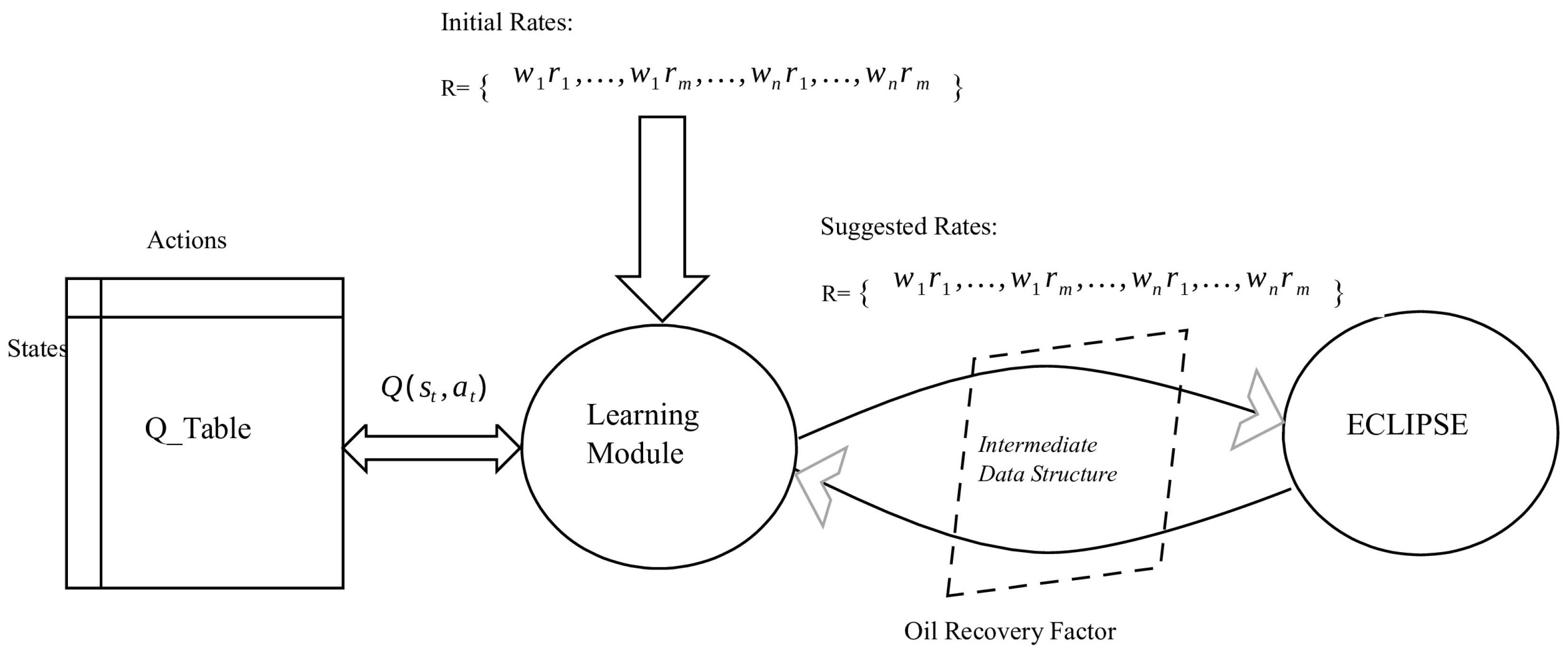
The overall architecture of the proposed system is depicted in Figure 2. The process begins with an initial well-rate set, $R=w_1{r}_1,\dots ,w_1{r}_m,\dots ,w_n{r}_1,\dots ,w_n{r}_m$, which is provided by an expert and inputted into the system. These rates are then passed to the ECLIPSE reservoir simulator.

The system then treats the initial well-rate set as a baseline and initiates a new episode. Using the Q-table and the current state, the system randomly selects a permissible new action or chooses a previously tried one based on the $ϵ-greedy$ algorithm. It updates the reward table by assigning a reward to the chosen action. Once all wells have been addressed, the episode concludes.

The resulting well-rate set is passed to the ECLIPSE simulator, which returns the corresponding oil recovery factor. This value is compared with previous amounts, and a positive or negative reward is assigned for higher or lower amounts, respectively. The process repeats iteratively until the system converges to an acceptable oil recovery factor.

To prevent redundant simulator runs, an $IntermediateDataStructure$ is introduced. It records the chosen well-rate and the resulting oil recovery factor, eliminating the need for repetitive simulations.

3. Evaluation of the Method

The objective of the proposed method is to provide effective input rates for each well within a reservoir in order to optimize the oil recovery factor. The system engages with the reservoir simulator and incrementally enhances the input rate set based on the Q-learning algorithm. To assess the efficacy of the proposed method, an experiment is conducted in the oil reservoir domain.

3.1. Experimental Setup

In this study, the Eclipse 100 reservoir simulator is chosen to synchronize with the Q-learning (QL) algorithm. Eclipse 100 is a fully implicit, three-phase, three-dimensional black oil simulator with a gas condensate option. It is implemented in FORTRAN 77 and can run on any computer with an ANSI-standard FORTRAN 77 compiler and sufficient memory [20].

The ECLIPSE simulator supports standard input data files containing reservoir characteristics and other required information for reservoir simulation. For our experiment, we utilize the SPE9 reservoir model, which is a three-dimensional black oil reservoir model. The SPE9 model consists of 26 wells, including 25 oil-producing wells and 1 injection well. However, for the purpose of our experiment, the reservoir is simplified to include only 2 producing wells and 1 injection well. We must emphasize that the choice of well locations has no impact on the process. These instances are merely examples that can be subject to change. Any number of wells in any spatial configuration provided as output by simulators can be utilized by the new method.

Figure 3 illustrates the simplified SPE9 reservoir model used in our study. It comprises 15 layers, each with a thickness of 24.25. The grid blocks are rectangular, with dimensions of 300 feet in both the x and y directions. The top layer has a depth of 9000 feet below sea level, and the porosity remains constant within each layer. The oil-water contact is at a depth of 9950 feet below sea level. In the base case, the injection well operates at a constant rate of 10,000, while the production wells have a rate of 4500. However, in this case study, the production rates are allowed to vary among 4400 barrels, 4500 barrels, and 4600 barrels, while for the injection well, the rates can vary among 9900 barrels, 10,000 barrels, and 10,100 barrels. The specific range of rates was determined by a reservoir engineer for this particular small-scale case study.

3.2. Results

The evaluation experiment focuses on the Q-learning method’s capability to improve the oil recovery factor.

The proposed model runs with initial rates from an expert and converges to a fixed value after enough iterations. The primary estimation from the reservoir engineer is 0.047407. The system runs for four iteration numbers, 100, 500, 1000, and 5000, and the experiment is repeated ten times each time. The system is completely trained in 500, 1000, and 5000 iterations and converges to a fixed value. Figure 4 shows the model training and converging graph for 1000 iterations. The result shows that the system converged to the fixed number of 0.047427 for the oil recovery factor after enough iterations. This indicates the reinforcement learning capability to learn the reservoir environment.

The evaluation experiment focuses on assessing the ability of the Q-learning method to enhance the oil recovery factor. The proposed model is initialized with initial rates provided by an expert and undergoes multiple iterations until convergence to a fixed value is achieved. The reservoir engineer’s initial estimation for the oil recovery factor is 0.047407. The experiment is conducted for four different iteration numbers: 100, 500, 1000, and 5000, with each experiment repeated ten times.

The system demonstrates improvement as the number of iterations increases, ultimately converging to a fixed value. The model is fully trained within 500, 1000, and 5000 iterations, reaching a stable state. Figure 4 depicts the training and convergence graph for 1000 iterations, illustrating how the system progressively converges to an oil recovery factor of 0.047427. This showcases the capability of reinforcement learning to understand and adapt to the reservoir environment.

Figure 5 presents the comparison of the oil recovery factor (FOE) over time. The solid line represents the results obtained from the proposed model, while the dashed line represents the FOE resulting from the initial well-rate set provided by the expert. The results consistently indicate an increased oil recovery factor across all time intervals when the proposed model is applied. This demonstrates the effectiveness of reinforcement learning in improving the oil recovery factor.

3.3. Analysis and Discussion

In this section, we analyze and interpret the results obtained from the experiment and discuss the implications and significance of the obtained results within the broader context of the research field. We examine the convergence of the model, the improvement over the expert’s initial rates, and the reinforcement learning capabilities. We also explore potential future research directions and acknowledge the limitations of the study.

3.3.1. Convergence of the Model

The proposed model demonstrates convergence to a fixed value after a sufficient number of iterations. For the experiment conducted, the system runs for four different iteration numbers: 100, 500, 1000, and 5000. After running the experiment ten times for each iteration number, it is observed that the model converges to a fixed value. Figure 4 illustrates the model training and converging graph for 1000 iterations, showing a clear convergence trend. The obtained results indicate the reinforcement learning capability of the model to learn the reservoir environment.

3.3.2. Improvement over Initial Rates

The primary estimation of the oil recovery factor from the reservoir engineer was 0.047407. By applying the proposed model, the system achieves an improvement in the oil recovery factor. The model is trained for different iteration numbers, and the results demonstrate that the system converges to a fixed number after a sufficient number of iterations. The oil recovery factor reaches a value of 0.047427, indicating an improvement over the initial rates provided by the expert. This suggests the effectiveness of the proposed model in optimizing the oil recovery factor.

3.3.3. Implications of the Results

The results of the experiment provide evidence of the effectiveness of the proposed model in optimizing the oil recovery factor. By iteratively improving the input rate set using the Q-learning algorithm, the system demonstrates the ability to learn from the reservoir simulator and converge to an optimized solution. This has practical implications for the oil reservoir domain, as it offers a method to efficiently determine input rates for each well to enhance oil recovery.

3.3.4. Future Research Directions

While the current study focused on a simulated simplified oil reservoir, there are opportunities for further research. One potential direction is to explore the application of the proposed model on real data from actual oil reservoirs. This would allow for the evaluation of the model’s performance in more complex and larger-scale scenarios. Additionally, investigating the effect of removing the limitation on well access by utilizing computational geometry could be another interesting avenue for future study.

3.3.5. Limitations

The experiment was conducted on a simplified oil reservoir model, which may not fully capture the complexities of real-world reservoirs. The results obtained from this study should be interpreted within the context of these simplifications. Further validation and testing on a wider range of reservoir scenarios are necessary to establish the robustness and generalizability of the proposed model.

4. Conclusions

In conclusion, this paper presented a model for optimizing the oil recovery factor in reservoirs using the Q-learning algorithm. The proposed model demonstrated its capability to improve the oil recovery factor through iterative interactions with a reservoir simulator. The results indicated the effectiveness of the reinforcement learning approach in optimizing input rates for each well.

The findings of this study contribute to the field of reservoir optimization and highlight the potential of using reinforcement learning techniques in the oil industry. The proposed model shows promise for improving oil recovery and can serve as a basis for further research and development in this area.