
Anomaly Recognition, Diagnosis and Prediction of Massive Data Flow Based on Time-GAN and DBSCAN for Power Dispatching Automation System


Abstract
:1. Introduction
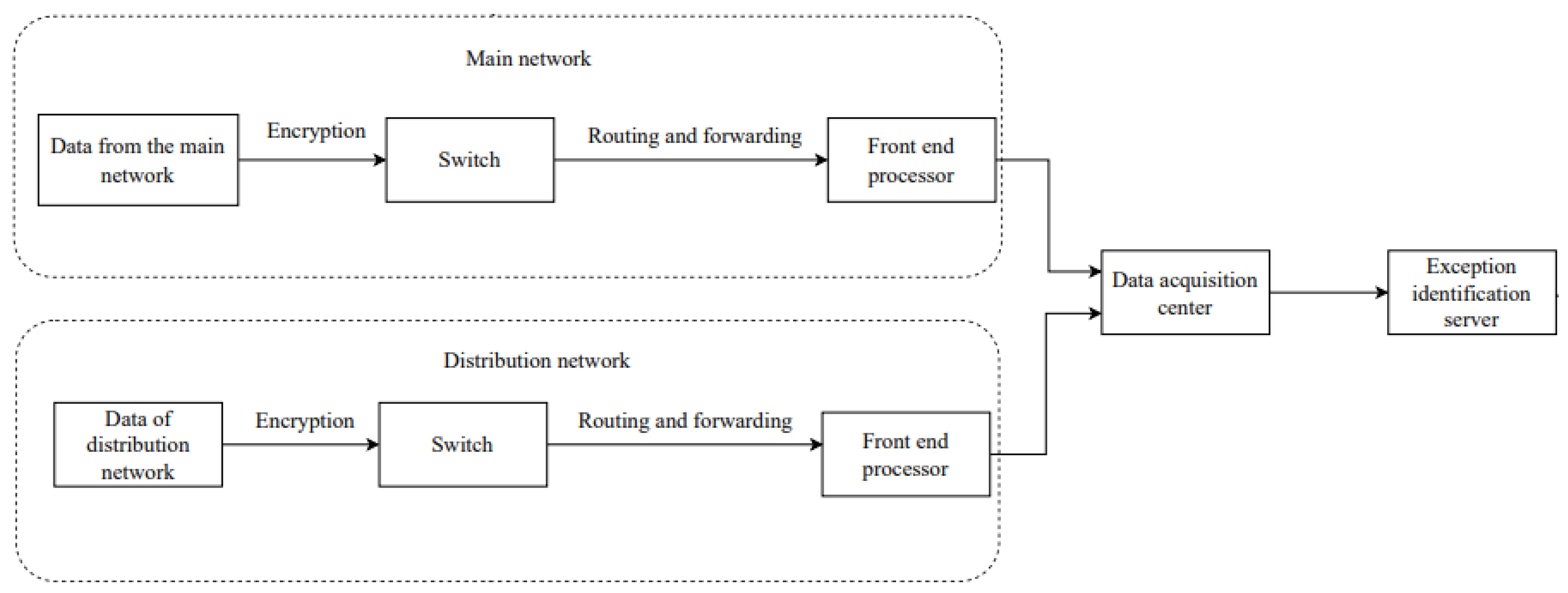
2. System Model
2.1. Power Dispatching Automatic System
2.2. Anomaly Classification of Scheduling Service Information Flow
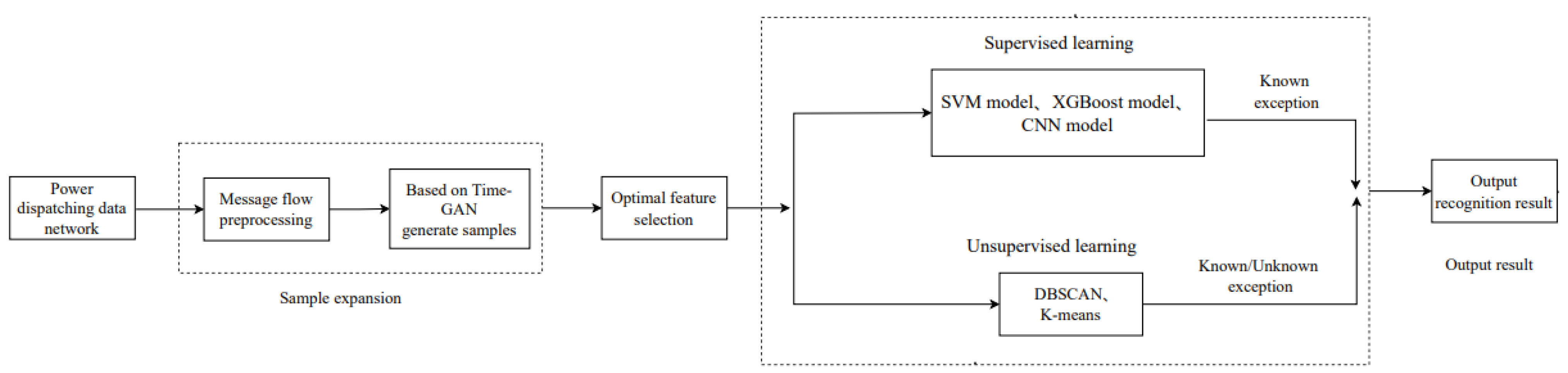
2.3. Abnormal Characteristics and Fault Identification Process Based on Massive Information Flow
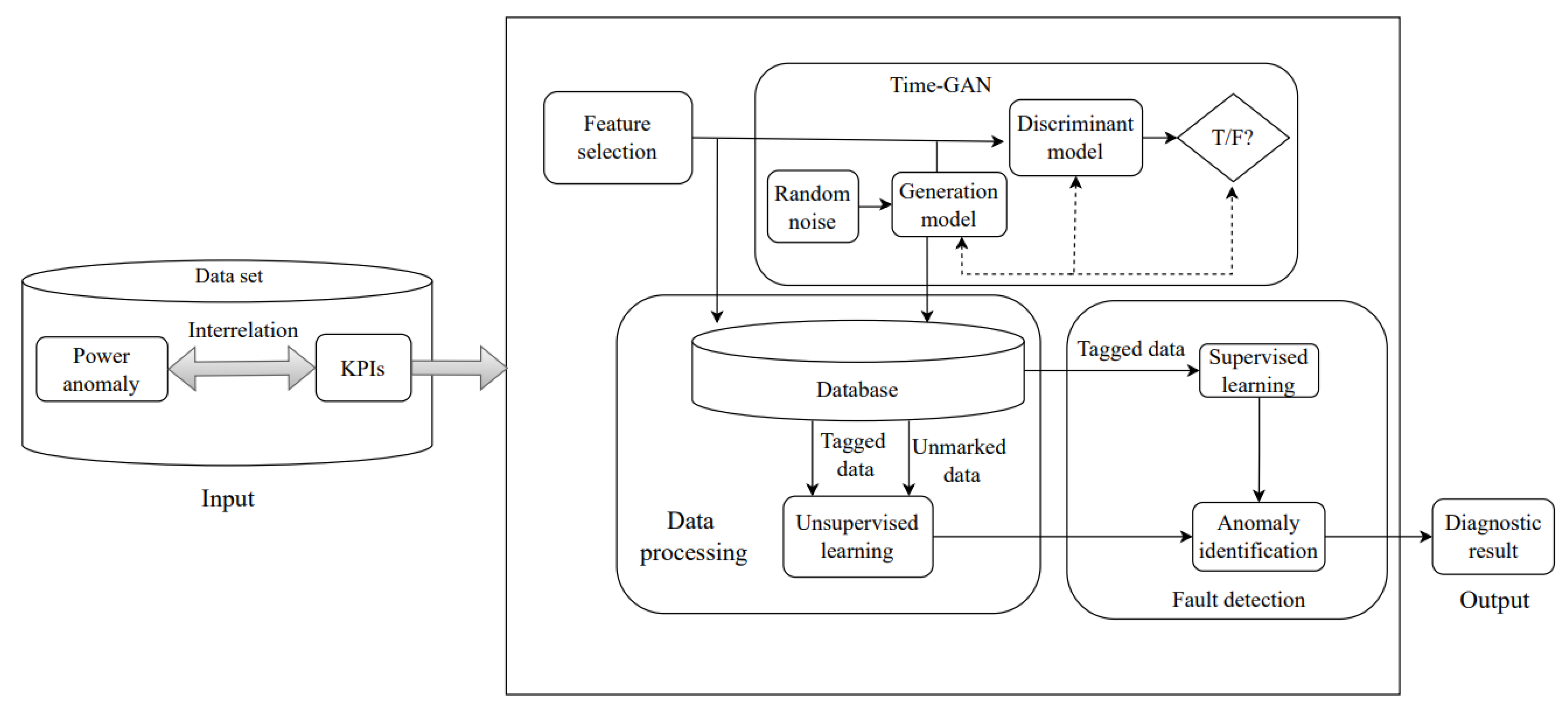
3. System Fault Diagnosis and Prediction Based on Time-GAN and DBSCAN
3.1. Data Generation by Time-GAN
| Algorithm 1 Time-GAN Algorithm [14] |
| 1 Input: , training set , input size per batch , learning rate 2 Initialization: 3 while generator does not converge do 4 Transformation between feature space and latent space 5 Sample 6 for do 7 8 9 Generate latent space codes 10 Sample 11 for do 12 13 Discrimination between real data and synthetic data 14 for do 15 16 17 Calculate reconstruction loss, unsupervised and supervised loss 18 19 20 21 Update by gradient operator 22 23 24 25 26 Generate synthetic data 27 Sample 28 Generate synthetic hidden space codes 29 for do 30 31 Convert latent space code to feature space 32 for do 33 34 end while 35 output: |
3.2. DBSCAN Algorithm
| Algorithm 2 DBSCAN algorithm [15] |
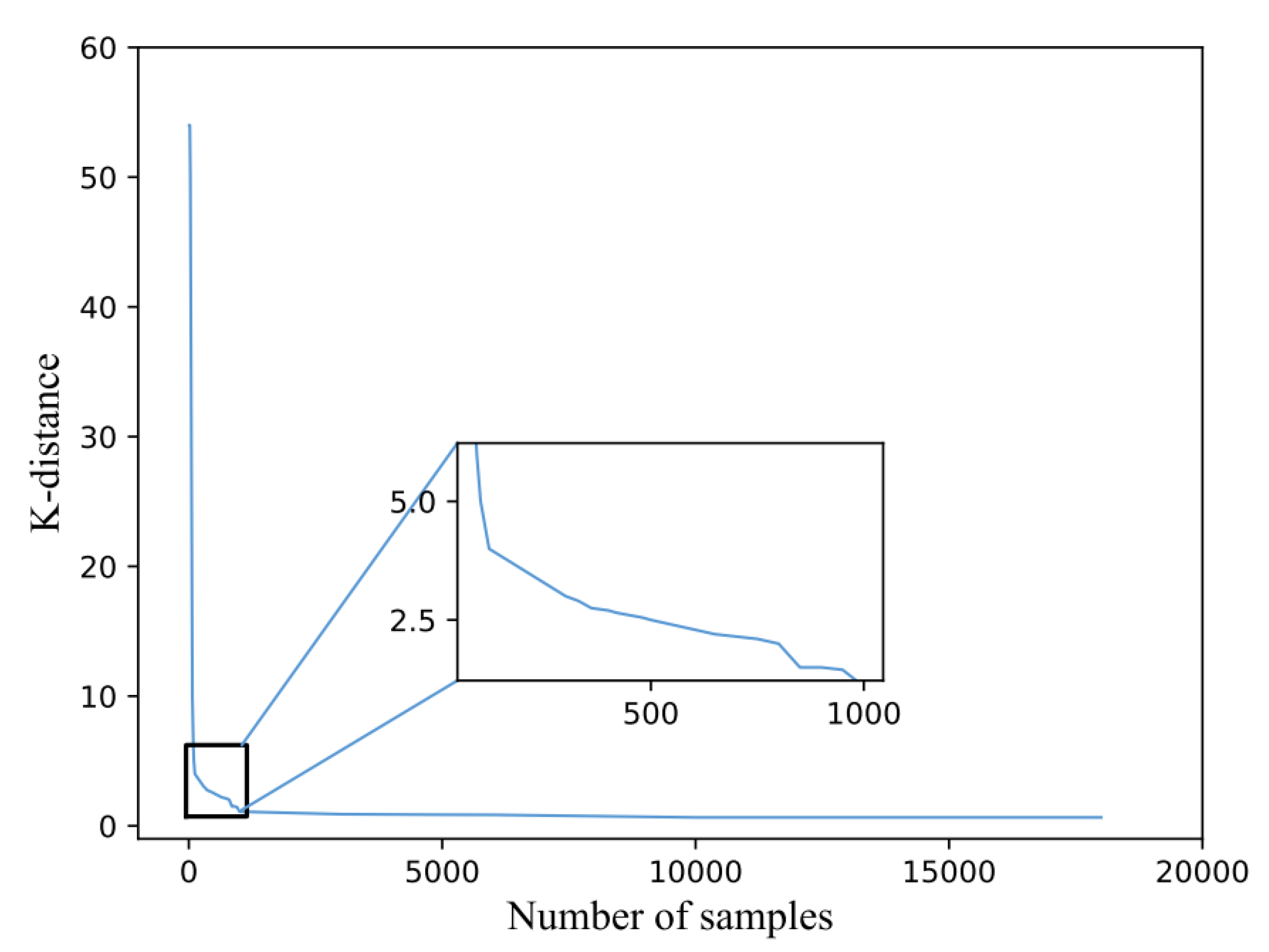
| 1 Input: dataset D containing n objects, radius parameter ε, minimum number of samples μ 2 Initialization: ε = 2.5, μ = 14, Cluster list[ ] 3 Set the cluster classification tag D.cluster of data in the dataset as unclustered 4 For i , do 5 If there are at least μ samples within the domain radius ε of (whether the sample is a core instance) 6 Create a new cluster C, add C to the Cluster list[ ], and add to C 7 Take all samples in the ε-neighborhood radius of to form a set N (N is consisted of ) 8 for each sample in N 9 mark as clustered 10 If there are at least μ samples within the neighborhood radius ε 11 Add sample to C 12 If does not belong to C 13 Set the cluster classification tag D.cluster of data in the dataset as unclustered 14 End while 15 Data that are still marked as unclustered are classified as outliers, marked as −1 and placed in the Cluster 16 list[] 17 Output: the samples tagged as unclustered |
4. Performance Analysis
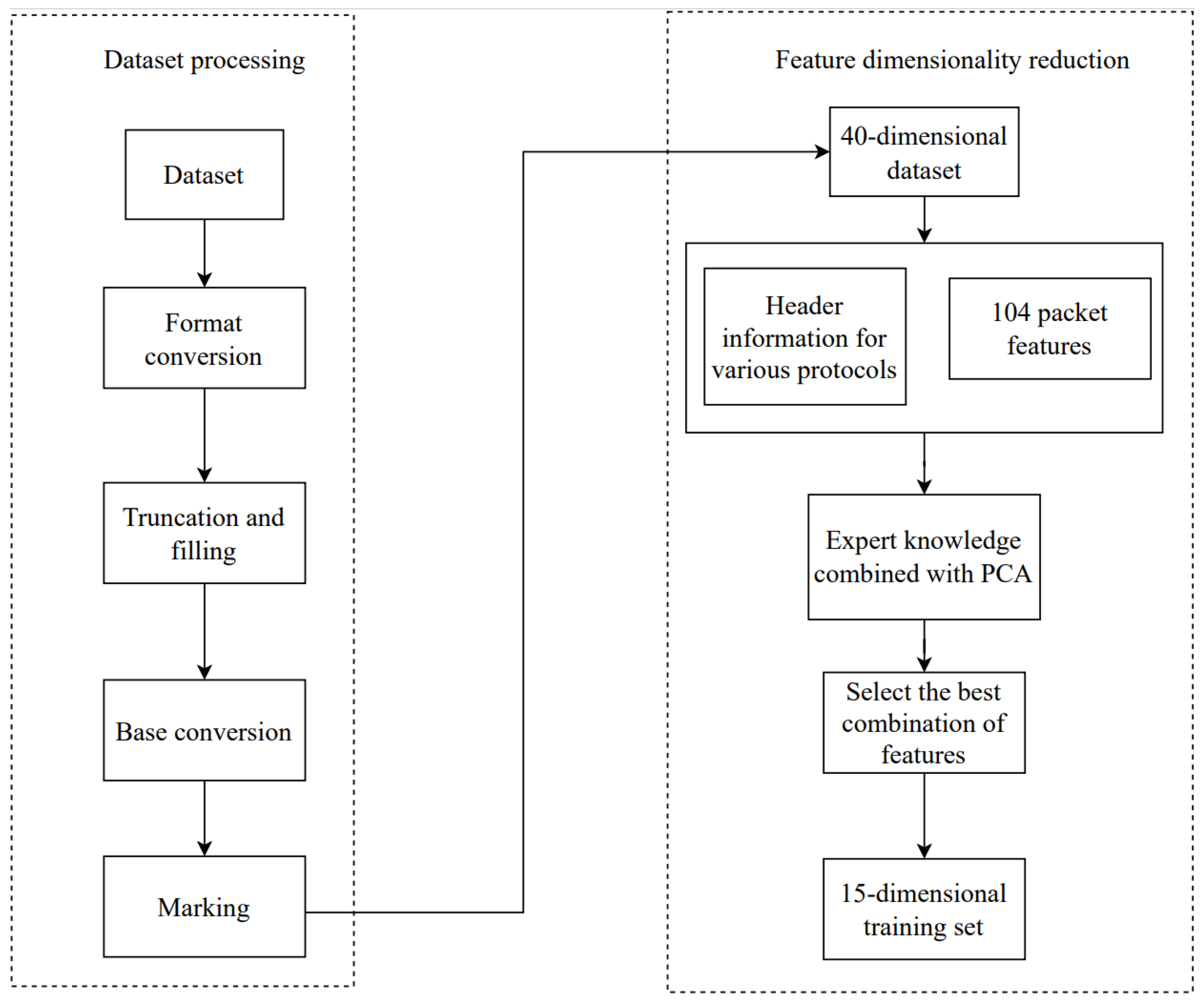
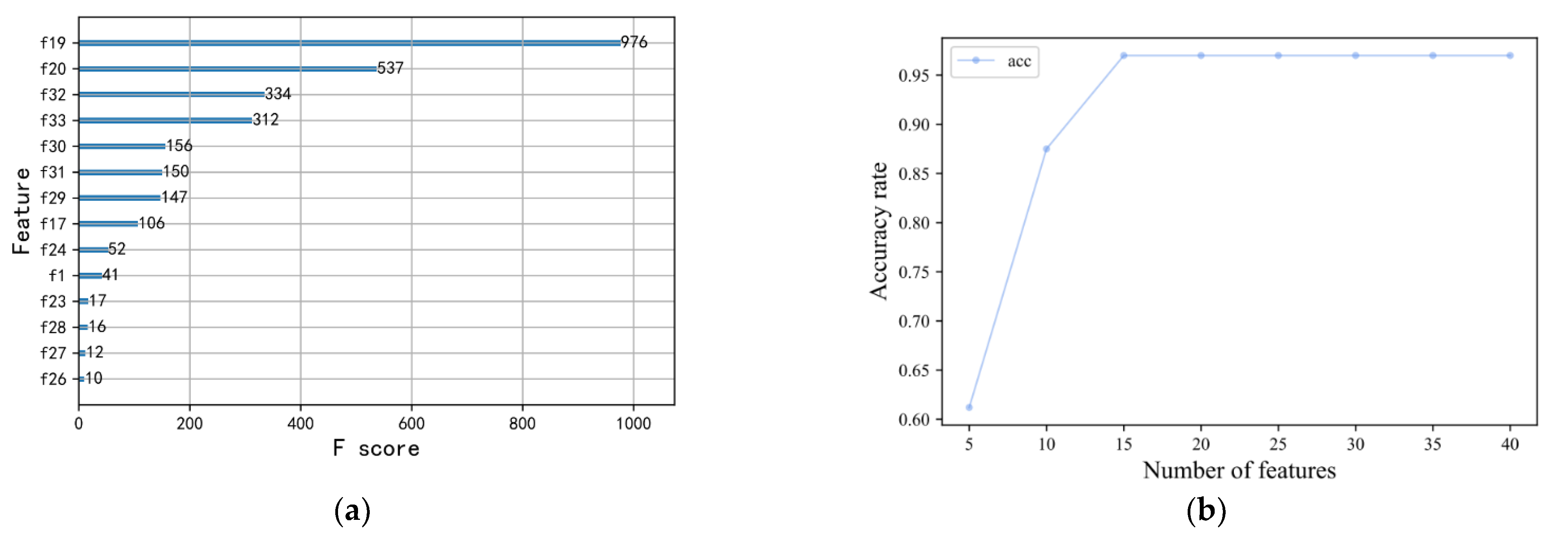
4.1. Optimal Feature Selection
4.2. Comparison of Accuracy of Various Algorithms on Known Anomalies
4.3. Comparison of Accuracy of Various Algorithms on Unknown Anomalies
4.4. Unknown Anomaly Detection
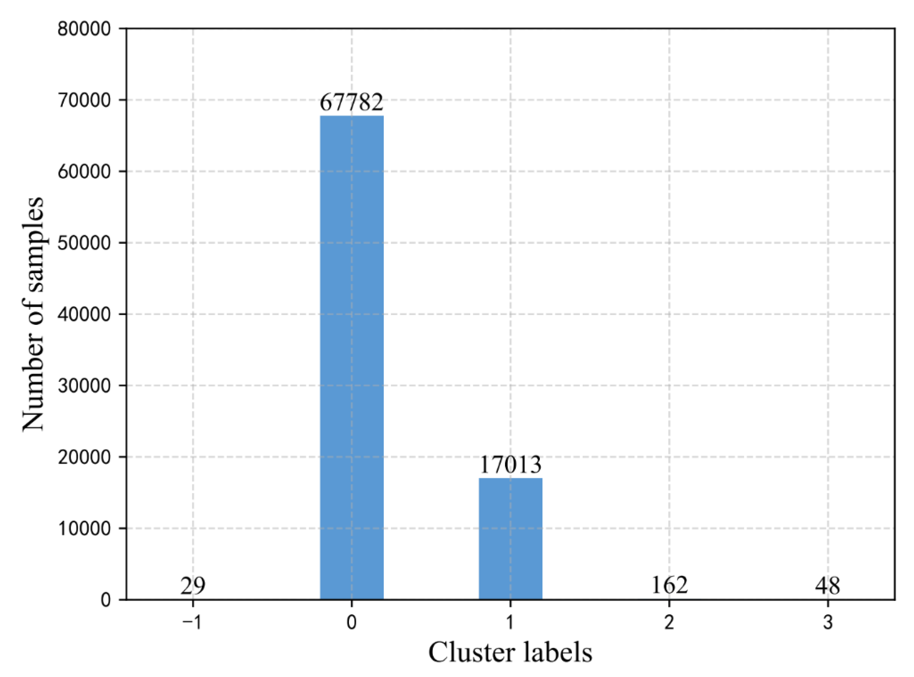
4.4.1. Applying DBSCAN Algorithm to Detect Unknown Anomalies
4.4.2. Applying K-Means to Detect Unknown Anomalies
4.4.3. The Practical Application of the Algorithm
5. Conclusions
Author Contributions
Funding
Data Availability Statement
Conflicts of Interest
References
- Jian, F.; Cao, M.; Wang, L.; Sun, Z.; Zhang, J.; Wang, H. Research on Electrical anomaly Detection in AMI environment based on SV [基于SVM的AMI环境下用电异常检测研究]. Electr. Meas. Instrum. 2014, 51, 64–69. [Google Scholar]
- Xu, Y.; Li, S.; Han, Y. Abnormal power consumption behavior detection based on CNN-GS-SVM [基于CNN-GS-SVM的用户异常用电行为检测]. Control. Eng. China 2021, 28, 1989–1997. [Google Scholar]
- Yang, Z.; Ding, J.; Chen, G.; Kang, X.; Sheng, M. Research on Abnormal Power Consumption Detection Method of Power Big Data based on LightGBM and LSTM model [基于 LightGBM 和LSTM模型的电力大数据异常用电检测方法研究]. Electr. Instrum. Meas. 2023, 1–7. Available online: http://kns.cnki.net/kcms/detail/23.1202.TH.20220713.1958.004.html (accessed on 15 May 2023).
- Liu, D.; Jiang, Z.; Zhu, Y.; Huang, Y.; Xiao, Y. Abnormal detection of power monitoring system network traffic based on LDSAD [基于LDSAD的电力监控系统网络流量异常检测]. J. Zhejiang Electr. Power 2022, 9, 87–92. [Google Scholar] [CrossRef]
- Yan, Y.; Sheng, G.; Chen, Y.; Jiang, X.; Guo, Z.; Du, X. Abnormal detection method of state data of power transmission and transformation equipment based on big data analysis [基于大数据分析的输变电设备状态数据异常检测方法]. Proc. CSEE 2015, 35, 52–59. [Google Scholar]
- Huang, G.J. Research on Flow Data Analysis of power Enterprises based on Canopy-Kmeans algorithm [基于Canopy-Kmeans算法的电力企业流量数据分析研究]. Inf. Technol. Netw. Secur. 2022, 41, 5. [Google Scholar] [CrossRef]
- Wu, G.; Yao, J.; Guan, M.; Zhu, X.; Wu, K.; Li, H.; Song, S. Power transformer fault diagnosis based on DBSCAN [基于DBSCAN的电力变压器故障诊断]. J. Wuhan Univ. (Eng. Sci.) 2021, 54, 1172–1179. [Google Scholar]
- Wang, P.; Zhang, Q. Power expert fault diagnosis information fusion method based on fuzzy clustering [基于模糊聚类的电力专家故障诊断信息融合方法]. J. Heilongjiang Electr. Power 2020, 2, 109–112+118. [Google Scholar] [CrossRef]
- Dong, X.-Y. Research on Intrusion Detection Method of Wireless Network based on Clustering Algorithm [基于聚类算法的无线网络入侵检测方法研究]. Master’s Thesis, Hebei Normal University, Shijiazhuang, China, 2022. [Google Scholar] [CrossRef]
- Jian, S.; Lu, Z.; Jiang, B.; Liu, Y.; Liu, B. Traffic anomaly detection based on hierarchical clustering method. Inf. Secur. Res. 2020, 6, 474–481. [Google Scholar]
- Goodfellow, I.J.; Pouget-Abadie, J.; Mirza, M.; Xu, B.; Warde-Farley, D.; Ozair, S.; Courville, A.; Bengio, Y. Generative adversarial nets. In Proceedings of the International Conference on Neural Information Processing System/s, Montreal, QC, Canada, 8–13 December 2014; MIT Press: Cambridge, MA, USA, 2014; pp. 2672–2680. [Google Scholar]
- Arjovsky, M.; Bottou, L. Towards principled methods for training generative adversarial networks. arXiv 2017, arXiv:1701.04862. [Google Scholar]
- Liu, H.; Gu, X.; Samaras, D. Wasserstein GAN With Quadratic Transport Cost. In Proceedings of the 2019 IEEE/CVF International Conference on Computer Vision (ICCV), Seoul, Republic of Korea, 27 October–2 November 2019; pp. 4831–4840. [Google Scholar] [CrossRef]
- Yoon, J.; Jarrett, D.; Van der Schaar, M. Time-series generative adversarial networks. In Proceedings of the Neural Information Processing Systems (NeurIPS), Vancouver, BC, Canada, 8–14 December 2019. [Google Scholar]
- Ester, M.; Kriegel, H.P.; Sander, J.; Xu, X. A Density-Based Algorithm for Discovering Clusters in Large Spatial Databases with Noise. In Proceedings of the 2nd International Conference on Knowledge Discovery and Data Mining, Portland, OR, USA, 2–4 August 1996. [Google Scholar]


| KPI Parameters | Symbolic | KPI Parameters | Symbolic |
|---|---|---|---|
| 104 message | 104_M | TCP Keep-Alive message explosion | TCP_KA_E |
| Type ID | TY | The number of retransmission packets exploded | RET_E |
| Timestamp | TS | Remote letters explosion | RL_E |
| Telemetry message explosion | TM_E | Status value | SV |
| Anomaly Classification | Representational Phenomenon | KPI |
|---|---|---|
| Device reboot error | A large number of devices restart recovery | 104_M, TY, TS, TCP_KA_E |
| Device Alternate Channel Error | Can’t connect to backup channel | 104_M, TY, TS, TCP_KA_E, RET_E |
| telemetry error | Collective telemetry upload | 104_M, TY, TS, TM_E |
| Total call error | The total summoning frequency is abnormal | 104_M, TY, TS, TCP_KA_E |
| Generating Algorithm | Classic GAN | WGAN | Time-GAN |
|---|---|---|---|
| Optimal generation ratio | 1:1 | 1:2.1 | 1:4 |
| Generating model accuracy | 0.93 | 0.96 | 1 |
| Generating model precision | 0.92 | 0.96 | 1 |
| Generating model recall | 0.94 | 0.96 | 1 |
| SVM | XGBoost | CNN | DBSCAN | K-Means | |
|---|---|---|---|---|---|
| Device restart error | 0.12 | 1 | 0.92 | 1 | 0.37 |
| Communication interruption | 0.74 | 0.65 | 0.72 | 1 | 0.45 |
| Collective telemetry upload | 0.23 | 0.52 | 0.82 | 1 | 0.76 |
| Total call error | 0.46 | 0.92 | 1 | 1 | 0.49 |
| Length | Control Bit 1 | Control Bit 2 | Control Bit 3 | Control Bit 4 | Send Reason | Address 1 | Address 2 | Telemetry Value 1 | Telemetry Value 2 | Cluster Class |
|---|---|---|---|---|---|---|---|---|---|---|
| 70 | 60 | 58 | 238 | 9 | 3 | 12 | 64 | 99 | 122 | −1 |
| 154 | 22 | 124 | 242 | 9 | 3 | 7 | 64 | 0 | 0 | −1 |
| 124 | 88 | 235 | 244 | 9 | 3 | 145 | 64 | 46 | 9 | −1 |
| APDU Length | Type ID | Transmission Reason | ASDU Public Address | Information Object Address | Telemetry Value |
|---|---|---|---|---|---|
| 58 | 9 | 3 | 1 | 0x4001 | 10,441 |
| 58 | 9 | 3 | 1 | 0x4039 | 10,462 |
| 64 | 9 | 3 | 1 | 0x4037 | 10,442 |
| 64 | 9 | 3 | 1 | 0x4037 | 10,458 |
| 64 | 9 | 3 | 1 | 0x4037 | 10,431 |
Disclaimer/Publisher’s Note: The statements, opinions and data contained in all publications are solely those of the individual author(s) and contributor(s) and not of MDPI and/or the editor(s). MDPI and/or the editor(s) disclaim responsibility for any injury to people or property resulting from any ideas, methods, instructions or products referred to in the content. |
© 2023 by the authors. Licensee MDPI, Basel, Switzerland. This article is an open access article distributed under the terms and conditions of the Creative Commons Attribution (CC BY) license (https://creativecommons.org/licenses/by/4.0/).
Share and Cite
Liu, W.; Lei, P.; Xu, D.; Zhu, X. Anomaly Recognition, Diagnosis and Prediction of Massive Data Flow Based on Time-GAN and DBSCAN for Power Dispatching Automation System. Processes 2023, 11, 2782. https://doi.org/10.3390/pr11092782
Liu W, Lei P, Xu D, Zhu X. Anomaly Recognition, Diagnosis and Prediction of Massive Data Flow Based on Time-GAN and DBSCAN for Power Dispatching Automation System. Processes. 2023; 11(9):2782. https://doi.org/10.3390/pr11092782
Chicago/Turabian StyleLiu, Wenjie, Pengfei Lei, Dong Xu, and Xiaorong Zhu. 2023. "Anomaly Recognition, Diagnosis and Prediction of Massive Data Flow Based on Time-GAN and DBSCAN for Power Dispatching Automation System" Processes 11, no. 9: 2782. https://doi.org/10.3390/pr11092782
APA StyleLiu, W., Lei, P., Xu, D., & Zhu, X. (2023). Anomaly Recognition, Diagnosis and Prediction of Massive Data Flow Based on Time-GAN and DBSCAN for Power Dispatching Automation System. Processes, 11(9), 2782. https://doi.org/10.3390/pr11092782