Research on a Carbon Emission Prediction Method for Oil Field Transfer Stations Based on an Improved Genetic Algorithm—The Decision Tree Algorithm

Abstract

The background of “dual carbon” is accelerating low-carbon transformation in the energy field, and oil field enterprises are facing challenges in energy conservation and emissions reduction for sustainable development. However, oil field gathering and transfer station systems, which are crucial components of the onshore transportation system, face challenges in energy conservation and emissions reduction. Therefore, it is necessary to predict the carbon emissions of oil field gathering and transfer station systems. To improve the accuracy of carbon emission prediction for the system, this study proposes an improved GA-decision tree (IGA-decision tree) algorithm. First, chaotic mapping was introduced to initialize the population, ensuring a uniform distribution of initial particles in the search space and enhancing population diversity. Second, the firefly perturbation strategy was employed to avoid the problem of genetic algorithms becoming trapped in local optima during the later stages of the search. The results show that the enhanced GA-decision tree algorithm effectively avoided being stuck in local optima while performing global searches. When predicting the carbon emissions of oil field gathering and transfer stations, the improved GA-decision tree (IGA-decision tree) algorithm outperformed traditional decision tree and GA-decision tree algorithms in terms of error and convergence efficiency. It achieved a root mean square error (RMSE) value of 74.5181 and a correlation coefficient (R²) of 0.99, indicating a high level of fitness and good convergence, as well as high prediction accuracy. This algorithm contributes to carbon accounting and energy conservation efforts in oilfield gathering and the transfer station system, filling the research gap in carbon emissions prediction for the system within the framework of energy internet projects.

1. Introduction

The oil industry is the basic industry of the Chinese national economy and energy security, and it is also an industry with high energy consumption, high pollution, and high carbon emissions. Since reform and opening up, the Chinese petroleum refining industry has developed rapidly, and the cumulative processing volume of China’s crude oil reached 703.554 million tons in December 2021, a cumulative increase of 4.3%, while the corresponding energy consumption and carbon emissions also showed a rapid growth trend. China has officially announced that it strives to achieve a carbon peak before 2030 and carbon neutrality before 2060. Under such circumstances, it is particularly important to accurately and efficiently grasp the carbon emissions level of enterprises in advance to provide strong support for the development of practical emission reduction pathways.

At present, research on carbon emissions prediction is mainly divided into three aspects. The first aspect is to combine historical data to establish a regression prediction model and estimate carbon emissions through several sets of statistical data. Wei et al. [1] analyzed the relationship between carbon dioxide emissions and influencing factors through correlation analysis and then used the optimized least squares support vector machine to predict carbon emissions, which effectively improved the prediction accuracy of carbon emissions. Faruque et al. [2] established a prediction model for the impact of carbon dioxide emissions on electric consumption and gross domestic product (GDP) and compared and analyzed the prediction accuracy of four deep learning methods: convolutional neural network (CNN), convolutional neural network-long short-term memory (CNN-LSTM), LSTM and dense neural network (DNN). Chen et al. [3], based on private car trajectory data, using inverse geocoding and an artificial neural network to predict the carbon emissions of private cars in various regions, also evaluated the emissions reduction potential of various regions from the perspectives of efficiency, effect, and fairness, which provided a reference for formulating emission reduction strategies in China’s road transportation field. The second aspect is to conduct scenario analysis or establish a carbon peaking prediction model to predict the carbon peaking situation of various industries. Xu et al. [4] built a top-down energy system model of China’s civil aviation industry based on LEAP (Long-Range Energy Alternatives Planning System) and discussed the technical path of low-carbon development in the civil aviation industry in the medium and long term, including how the number of flights is expected to quadruple in China by 2060, and under the current policy scenario, carbon emissions from the civil aviation industry are expected to peak at around 2046, with a peak level of about 350 million tons. Li et al. [5] firstly used Kaya identity and the logarithmic mean Di exponential decomposition method (LMDI) to decompose the influencing factors of carbon emissions from civil aviation transportation in China; secondly, a Tapio decoupling model was established to analyze the correlation between carbon emissions of civil aviation transport and various influencing factors; and finally, the improved and scalable STURBANAT model is used to realize the carbon emissions prediction of China’s civil aviation transportation, and it is expected that there will be no peak carbon emissions before 2050 under the baseline scenario. The third aspect is to establish a time series forecasting model with the help of computer deep learning and other methods to conduct the short-term or medium-term prediction of carbon emissions. Hu et al. [6] predicted the trend of carbon emissions intensity in China based on an LSTM neural network model. At the same time, the ARIMA-BP neural network model was established as a validation model to directly predict carbon emissions intensity, and the prediction results of these two models differed by 2.03 percentage points.

For the analysis of carbon emission reduction pathways, the existing research mainly uses scenario analysis methods on the basis of carbon emissions prediction to explore the carbon peak time and carbon emissions reduction potential under different paths by setting different scenarios. Stan [7] used the LEAP model, coupled with the logarithmic mean Diehlschild decomposition model, and used the scenario analysis method to predict the carbon peak time of Jiangsu Province under different scenarios. Bian [8] constructed a dynamic model of the carbon emissions system and set up six scenarios to simulate and predict the carbon peak time and emissions reduction potential of the Beijing–Tianjin–Hebei region. Liu [9], based on the PLS-VIP algorithm, studied 10 influencing factors related to carbon emissions for PLS (partial least squares) modeling as independent variables; the results showed that the proposed method could effectively identify the variables with a strong correlation to the dependent variable and fundamentally reduce the number of variables entering the model. Wang et al. [10] studied the influencing factors of the carbon emissions allowance price, constructed the graph structure of the index based on the complex network theory, and then established the graph structure adaptive Lasso method (G-AdLasso) to identify the influencing factors, and found that G-AdLasso could identify the more important indicators in the graph’s structure, and it is clear that this method can optimize and refine the model. Ke et al. [11] solved the problem of nonlinearity and instability of carbon emission data in order to use time series data information to predict carbon emissions more comprehensively, and the BAS-LSTM model of quadratic decomposition was used to predict the carbon emissions of Shaanxi Province. Gao et al. [12] established a support vector machine (GA-SVR) prediction model optimized by a genetic algorithm to predict the future carbon emissions of Beijing’s transportation industry; the results showed that there was a good fitting regression effect between the data obtained by the model and the actual value. Some scholars use neural network correlation methods to predict future carbon emission trends and, from the model prediction results, the neural network correlation method can predict future carbon emissions more accurately, which provides a quantitative basis for the city’s low-carbon planning and control of carbon emissions [13,14,15,16] at a regional level. Zhou [17] proposed a grey rolling prediction model, which considered the influence of new information on development trends and improved the accuracy and stability of predictions. YU [18] proposed a multi-objective optimization model for economic carbon emissions costs to predict China’s energy structure, and the results show that carbon emission peaks can be reached between 2025 and 2028. Yan [19] used the STIRPAT model to predict carbon emissions in the blue economic zone of the Shandong Peninsula, and the relationship between population, energy intensity, and carbon emissions was analyzed by the ridge regression method. At the industry level, many scholars have studied the timing of carbon emissions peaking in industries such as electricity [20], transportation [21], construction [22], and industry [23] and control measures to promote carbon peaking. Some authors [24,25,26,27,28,29] argue that population levels are strongly correlated with CO₂ emission levels. Al-Majidi [30] proposed a bacterial foraging algorithm (BF), which was employed to enhance the learning of the NN model for AGCs based on adequately identifying the initial weights of the model. Al-Majidi [31] proposed an artificial neural network (ANN) technique, which was utilized to design the optimal LFC.

In order to establish an accurate carbon emissions prediction model for the oil field transfer station, we selected variables such as daily power consumption, daily air consumption, and heat energy provided for analysis [32]. We optimized this model using the IGA-decision tree method and improved the accuracy of prediction by globally optimizing decision tree model parameters through the genetic algorithm.

There are many existing carbon emission prediction methods, and carbon emission prediction models have become a research hotspot, while traditional classical forecasting methods include single model methods, such as decision trees and support vector machines. However, there are some problems such as unstable regression and uncertain influencing factors, which make it difficult to predict carbon emissions scientifically and accurately. Therefore, in view of the shortcomings of traditional carbon emission prediction methods, this paper used the IGA-decision tree method to establish a carbon emissions prediction model for oilfield transfer stations to improve the accuracy of prediction.

The oil industry is a basic industry, and it holds significant importance in the context of carbon peaking and carbon neutrality. It is crucial to establish and implement emission reduction pathways for the oil industry in order to align with these objectives. Energy conservation and emission reduction can effectively reduce energy consumption in the actual production process of oilfield enterprises, thereby producing and processing more oil and gas resources. This enhances the economic benefits of oil field enterprises and achieves sustainable development. By combining the actual conditions of the oil field, implementing emission reduction measures, and establishing an evaluation and assessment system for energy conservation, water conservation, and clean production, we could establish a benchmark for building energy-efficient enterprises. This system evaluates and assesses the indicators related to energy conservation, water conservation, and clean production, thereby promoting sustainable development in the oil field industry. Vigorously adopting and actively implementing application-oriented and energy-efficient equipment is beneficial for improving energy utilization efficiency and achieving the goal of skill-based emissions reduction [33].

2. Methods Section

2.1. Measurement of Carbon Emissions

The oil field transfer station system is a crucial component in the oil production process, responsible for transporting crude oil from wells to gathering pipelines or storage tanks. However, this process inevitably generates a significant amount of carbon emissions. The oil field transfer station system requires the use of energy supply equipment, such as compressors and pumps, as well as control and transmission devices, during its operation. These devices typically rely on the combustion of fossil fuels, such as natural gas or diesel, which can lead to the emissions of greenhouse gases like carbon dioxide. In addition, the construction and maintenance of the oil field transfer station system also consumes a certain amount of energy and may generate some indirect carbon emissions.

The most important forms of carbon accounting can be divided into two methods: measurement-based and calculation-based, which can be summarized into three main methods: the measured method, emissions factor method, and mass balance method. Among these, the emissions factor method is the most widely applied and widely used carbon accounting method [11]. The carbon emission factors of each energy source are extrapolated based on data from research reports such as the 2005 China Greenhouse Gas Inventory Study and the 2006 IPCC Guidelines for National Greenhouse Gas Inventories. The carbon emissions accounting formula is as follows [3]:

CO₂ emissions from fossil fuel combustion are based on the amount of fuel burned by each combustion facility within the boundary, multiplied by the corresponding fuel carbon content and carbon oxidation rate. The carbon emissions of the furnace formula can be obtained as follows:

E_jrl = AD_jrl × CC_jrl × OF_jrl × 44/12

(1)

where E_jrl is the CO₂ emissions of the heating furnace, tCO₂; AD_jrl is the fuel consumption of the furnace, t or ten thousand Nm³; CC_jrl is the average carbon content of the furnace fuel, tCO₂/t or tCO₂/ten thousand Nm³; OF_jrl is the carbon oxidation rate of the furnace fuel, and the value range is 0~1.

Fuel carbon oxidation rate: the carbon oxidation rate of liquid fuel can take a default value of 0.98; the carbon oxidation rate of gas fuel can take a default value of 0.99 [28]; the carbon oxidation rate of solid fuel can be found according to different fuels.

The carbon footprint of the pump unit is calculated as:

E_bjz = AD_bjz × EF

(2)

where E_bjz is the CO₂ emissions for pump units, tCO₂; AD_bjz is the electricity consumed for the pump, MW·h; EF is CO₂ emission factors for the electricity supply, tCO₂/(MW·h).

2.2. Carbon Emission Prediction Model Methods

2.2.1. Decision Tree Algorithm Fundamentals

The gradient-boosting decision tree, abbreviated as GBDT, belongs to one of the branches of the decision tree model. Its core idea is to take residual learning as the basis, optimize the gradient direction to form a large number of regression trees, and all the regression tree results are added to the final model. To reduce residuals iterating one after another while, at the same time, obtaining high-precision results, they are suitable for working with a variety of nonlinear data. The gradient-boosting algorithm based on boosting, proposed by Friedman [34], has been widely used in various fields. The gradient-boosting decision tree algorithm consists of multiple decision trees, and the value of the negative gradient of the loss function in the current model is used as an approximation of the residual value in the boosted tree to fit the regression decision tree [35]. The general steps of the GBDT algorithm are as follows:

(1)

Enter N training samples X, and set the relevant parameters, the number of iterations (N), F as a function space composed of all trees, $f_k$ as a single decision tree model, and the initial value = 0, The GBDT algorithm expression is as follows:

$$y_i^1={\displaystyle \sum _{k=1}^K{f}_k\left(x_i\right)}$$

(3)

where $x_i$ is the eith feature vector of the sample; k is the number of weak regression trees; $f_k\left(x_i\right)$ is the output value of the kth weak regression tree; $y_i^1$ is the final predicted value of the i sample.

(2)

Define the objective function of the GBDT algorithm as:

$$Obj={\displaystyle \sum _{i=1}^{n}l\left(y_i,y_i^1\right)}+{\displaystyle \sum _{k=1}^K\Omega \left(f_k\right)}$$

(4)

where $\Omega$ is the complexity of the decision tree; n is the total number of samples; l is the loss function; $y_i$ is the i sample’s truth value.

This complexity is defined by the regular term:

$$\Omega \left(f_t\right)=kT+\frac{1}{2}\lambda {\displaystyle \sum _{j=1}^T{w}_j^2}$$

(5)

where T is the number of nodes on the leaf; $w_j$ is the vector value corresponding to the leaf node; k is the minimum amount of loss reduction required for the leaf node splitting of the tree; $\lambda$ is the penalty term coefficient.

(3)

According to the additive structure of the GBDT algorithm:

$$y_i^t=y_i^{t-1}+f_t\left(x_i\right)$$

(6)

where $y_i^t$ is the sum of the outputs of the top t trees of the ith sample; $y_i^{t-1}$ is the sum of the outputs of the first for t − 1 trees in the ith sample; and $f_t\left(x_i\right)$ is the output value of the top t tree of the ith sample.

Substituting Equation (4) into the objective function and expanding it using Taylor yields:

$$Ob{j}^t={\displaystyle \sum _{i=1}^n\left[g_i{f}_t\left(x_i\right)+\frac{1}{2}{h}_i{f}_t^2\left(x_i\right)+kT+\frac{1}{2}\lambda {\displaystyle \sum _{j=1}^T{w}_j^2}\right]}={\displaystyle \sum _{j=1}^T\left[G_i{w}_j+\frac{1}{2}\left(H_i+\lambda \right)w_j^2\right]}+kT$$

(7)

where $G_i={\displaystyle \sum g_i}$, $H_i={\displaystyle \sum h_i}$, $g_i$ and $h_i$ is the first and second derivatives of the loss function, respectively.

Let the first derivative of $Ob{j}^t$ be 0; the optimal value of the leaf node can be obtained by $w_j^{\ast }$:

$$w_j^{\ast }=-\frac{G_j}{H_j+\lambda }$$

(8)

where $G_i$ is the sum of the first derivatives of loss function; $H_i$ is the sum of the second derivatives of the loss function; $\lambda$ is the penalty term coefficient.

The objective function value at this time was:

$$Obj=-\frac{1}{2}{\displaystyle \sum _{j=1}^T\frac{G_j^2}{H_j+\lambda }}+kT$$

(9)

where $Obj$ is the objective function; $G_i$ is the sum of the first derivatives of the loss function; $H_i$ is the sum of the second derivatives of the loss function; $\lambda$ is the penalty term coefficient; T is the number of nodes on the leaf; k is the minimum amount of loss reduction required for the leaf node splitting of the tree.

(4)

Generate a new decision tree through a greedy strategy to minimize the objective function value, and the optimal predicted value corresponding to the leaf node is obtained, $w_j^{\ast }$, add the newly generated decision tree $f_t\left(x\right)$ to the model, obtaining:

$$y_i^t=y_i^{t-1}+f_t\left(x_i\right)$$

(10)

where $y_i^t$ is the sum of the outputs of the top t trees of the ith sample; $y_i^{t-1}$ is the sum of the outputs of the first t − 1 trees in the ith sample; $f_t\left(x_i\right)$ is the output value of the top t tree in the ith sample.

(5)

Keep iterating until the end of N iterations, and the output of the GBDT algorithm is composed of N decision trees.

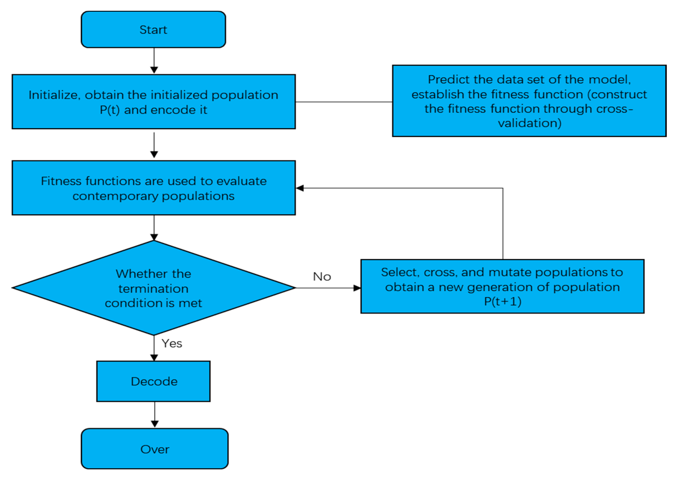
2.2.2. GA-Decision Tree Predictive Model Construction

A decision tree is a very representative algorithm in the field of machine learning, which can solve the classification problem and regression problem at the same time and has the characteristics of easy understanding and high computational efficiency. It is different from the integrated algorithms such as random forest and Adaboost, and a single decision tree often leads to the over-fitting of the model because of excessive division, especially when it trains small sample data sets. Aiming at the problem that the generalization ability of a single decision tree is not ideal, this paper proposes a decision tree regression model combining cross-validation and genetic algorithms (GA). Specifically, in the process of constructing decision tree branches, the maximum number of splits (MaxNumSplits), the minimum number of leaf size (MinLeafSize), and the minimum number of parent (MinParent) were the key superparameters that determined the degree of model splitting. The under-fitted model was set to young leads so that deep information in the training set could not be fully mined. When the setting was too large, the calculation often took a long time because of the deep layers of the tree, and the excessive split depth was also an important reason for the over-fitting of the model.

K-fold cross-validation is a practical method to cut data samples into smaller subsets statistically, which is mainly used in machine learning model training. In the given data sample, the training set was divided into K parts in equal quantities, and K − 1 copies were taken out in turn for modeling, while the remaining part of the sample was used to verify the established model and calculate the prediction error of this small part of the sample. Each time a different training set and test set were taken, the modeling was repeated K times, and the average prediction error of K models was used as the final model error. Since a certain sample was left for verification after each time modeling, the decision tree model based on K-fold cross-validation had strong overfitting resistance compared with the modeling method in which the whole training set participated in the training.

The genetic algorithm can be used to optimize the grid search to achieve global optimization. The GA algorithm and the decision tree model are connected by the fitness function, and the fitness function in this paper should be the average cross-validation error rate. It can be calculated from Equations (11) and (12):

$$Fi{t}^{*}=\frac{1}{K}{\displaystyle {\sum }_{i=1}^{K}fi{t}_i}$$

(11)

$$fi{t}_i=\frac{1}{N}{{\displaystyle {\sum }_{n=1}^{N_{}}(y_n-y{\prime }_n)}}^2$$

(12)

where $fi{t}_i$ represents the cross-validation error of the ith fold and represents the predicted MSE value of the validation fold; N is the number of samples per fold; $y_n$ and $y{\prime }_n$ represent the true and predicted values of the nth test sample in the validation compromise; $Fi{t}^{*}$ represents the mean cross-validation error, which is the final fitness function value.

The average cross-validation error rate is used as the fitness function to obtain the initialized population P(t), and then the selected population iteration can be carried out through the fitness function, and the selected genetic operator adopts the roulette method. The specific expression for this is as follows:

$$P_i=\frac{Fitnes{s}_i}{{\displaystyle \sum {}_{j=1}^{P}Fitnes{s}_j}}$$

(13)

where $P_i$ is the number of populations; $Fitnes{s}_i$ is the fitness value; ${\displaystyle \sum {}_{j=1}^{P}Fitnes{s}_j}$ is the total fitness value for the population, Selection through the fitness function can generate a new population P(t + 1), and the genetic operator operation continues on the basis of this population, operating in the order of selection, crossing, and mutation, and the selection is operated by roulette, leaving the individuals with high fitness behind while, on the contrary, low fitness is eliminated. Crossover is the following operation of individuals in a population:

$$\left\{\begin{array}{l}{x}^1=rx+\left(1-r\right)y\\ y^1=ry+\left(1-r\right)x\end{array}\right.$$

(14)

where x, y both represent the mother; $x^1,y^1$ represent two new individuals resulting from a maternal crossover; r is a random number between (0 and 1); nutation is the mutation operation of a gene in an individual:

$$\left\{\begin{array}{l}{x}_i^1=x_i+\left(b_i-x_i\right)f\left(g\right),i=j\&r_1<0.5\\ x_i^1=x_i+\left(a_i-x_i\right)f\left(g\right),i=j\&r_1\ge 0.5\\ x_i^1=x_i,otherwise\end{array}\right.$$

(15)

where $f\left(g\right)={\left(r_2\left(1-\frac{g}{K}\right)\right)}^k$, $r_1,r_2$ is a uniform random variable between (0 and 1); $j$ is a randomly selected variable; $g$ indicates the current generation; K represents the maximum number of iterations; i denotes the individual; $b_i,a_i$ indicates the next and previous sessions in the process of individual evolution; k represents a factor that decreases with the number of iterations.

After the operation of the above three genetic operators, the new population P(t + 2) was obtained; it is worth pointing out that this population was based on the hyperparameters of the decision tree prediction model. The specific process is shown in Figure 1:

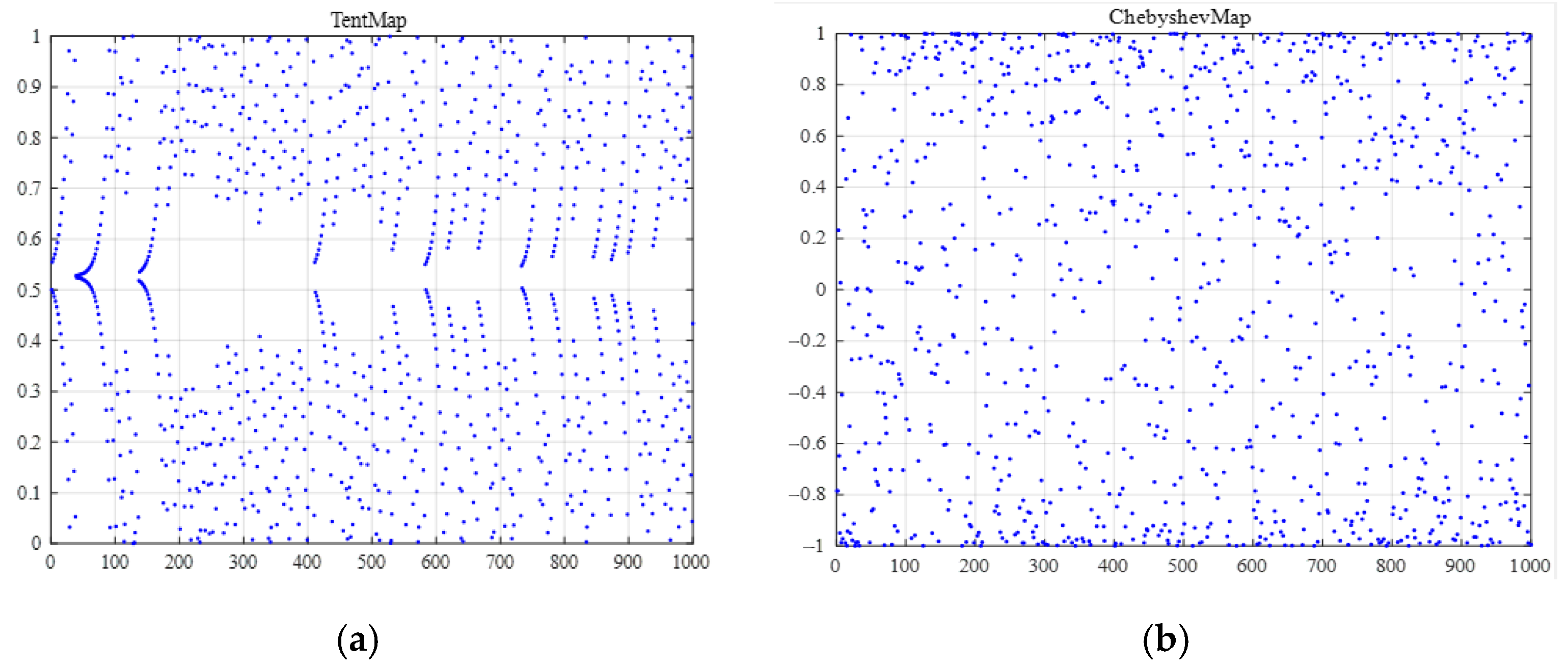
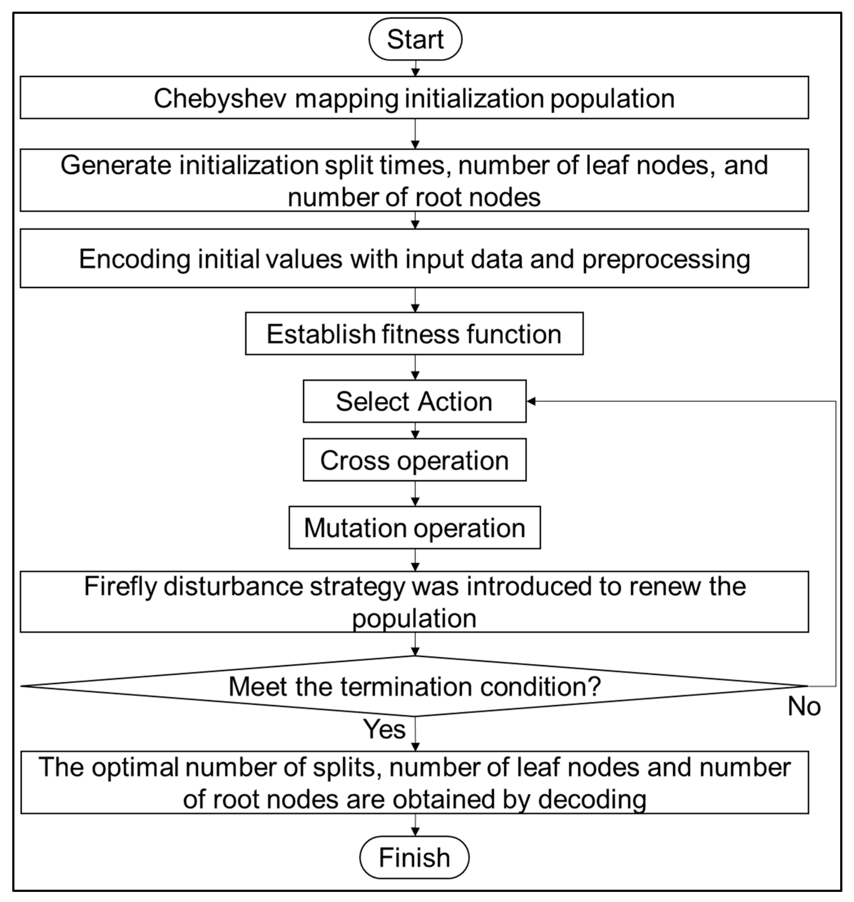
2.2.3. Establish an IGA-Decision Tree Algorithm Model

This model proposes two improvement strategies for the GA-decision tree algorithm. First, the population was initialized using Chebyshev chaotic maps to better cover the entire solution space with the initial chromosome; second, in response to the problem of genetic algorithm searching for the optimal individual in the later stage, which is prone to falling into local optima, a firefly disturbance strategy was introduced to modify it.

The standard genetic algorithm uses a random method to initialize the population, making it difficult to obtain stable target accuracy and convergence speeds during the search process. The more evenly distributed the initial population in the solution space, the greater the probability the algorithm has of finding the optimal value. Compared with random search strategies, chaotic search is widely used in the generation of initial populations due to its randomness and ergodicity.

The Firefly algorithm is a meta-heuristic algorithm proposed by Yang based on the flickering behavior of fireflies, characterized by its simple structure and global utilization ability [36]. In the genetic algorithm, specifically, chromosomes are equivalent to fireflies, and the distance between them and the optimal solution is denoted as $r_i=\left|x_i-x_{pot}\right|$·$x_{pot}$ represents the optimal individual and $x_i$ represents a random individual. Chromosomes guide population renewal through “luminescence”. The attractiveness of the optimal chromosome to an individual can be expressed as follows:

$$\zeta ={\zeta }_0\cdot \exp (-\gamma r_{i,j}^2)$$

(16)

where $\zeta$ is attractiveness; ${\zeta }_0$ is the maximum attraction, and can be related to the value of the objective function; $\gamma$ is the absorption coefficient of light intensity; $r_{i,j}$ is the spatial distance between firefly i and j.

The formula for updating the position of the population is as follows:

$$x_{newpot}=x_i+\zeta \cdot (x_i-x_{pot})+\alpha \cdot [rand(D)-0.5]$$

(17)

where α ∈ [0, 1] is a step size factor; $x_{pot}$ represents the optimal individual, $x_i$ represents a random individual; rand(D) ∈ [0, 1] is a random factor and is used to increase the search range and avoid entering local optima in later stages.

The steps for improving the GA-decision tree model are listed below:

This study used three parameters of decision tree optimization: the maximum number of splits, the minimum number of leaf nodes, and the minimum number of root nodes. The fitness function in this article should be the average cross-validation error rate, which can be calculated from Equations (18) and (19):

$$Fi{t}^{*}=\frac{1}{K}{\displaystyle {\sum }_{i=1}^{K}fi{t}_i}$$

(18)

$$fi{t}_i=\frac{1}{N}{{\displaystyle {\sum }_{q=1}^{N_{}}(y_q-y{\prime }_q)}}^2$$

(19)

where fit_i represents the cross-validation error of the i-th fold, and represents the predicted mse value of the validation fold; N is the number of samples per fold, y_q, and y′_q represent the true and predicted values of the qth test sample in the validation compromise; Fit* represents the average cross-validation error, which is the final fitness function value. The specific steps are as follows:

Step 1: Firstly, the Chebyshev chaotic map is used to initialize the population. The mathematical model of Chebyshev chaotic mapping is:

$$x(t+1)=\cos (t{\cos }^{-1}(x(t)))$$

(20)

where x(t) is the population individual at the tth iteration and x ∈ [−1, 1] while t is the current number of iterations. Tent chaotic mapping is the most commonly used population initialization method in the improvement process of intelligent optimization algorithms [37], and its results with Chebyshev chaotic mapping under a certain number of iterations are shown in Figure 2a,b. From Figure 2, it can be seen that compared to the Tent map, the initial population distribution generated by the Chebyshev map was more uniform, and the Chebyshev map had more efficient searchability when dealing with extreme problems.

Step 2: Generate the initial maximum number of splits, minimum number of leaf nodes, and minimum number of root nodes;

Step 3: Input data and preprocess to encode initial values;

Step 4: Establish a fitness function;

Step 5: Select the genetic, crossover, and mutation operations;

Step 6: Introduce a firefly disturbance strategy to update the population, determining whether the preset error conditions are met. If the conditions are met, the maximum number of splits, minimum number of leaf nodes, and minimum number of root nodes are output. If the conditions are not met, step 5 is revisited.

The main training process for improving the GA decision tree algorithm is shown in Figure 3:

3. Empirical Analysis

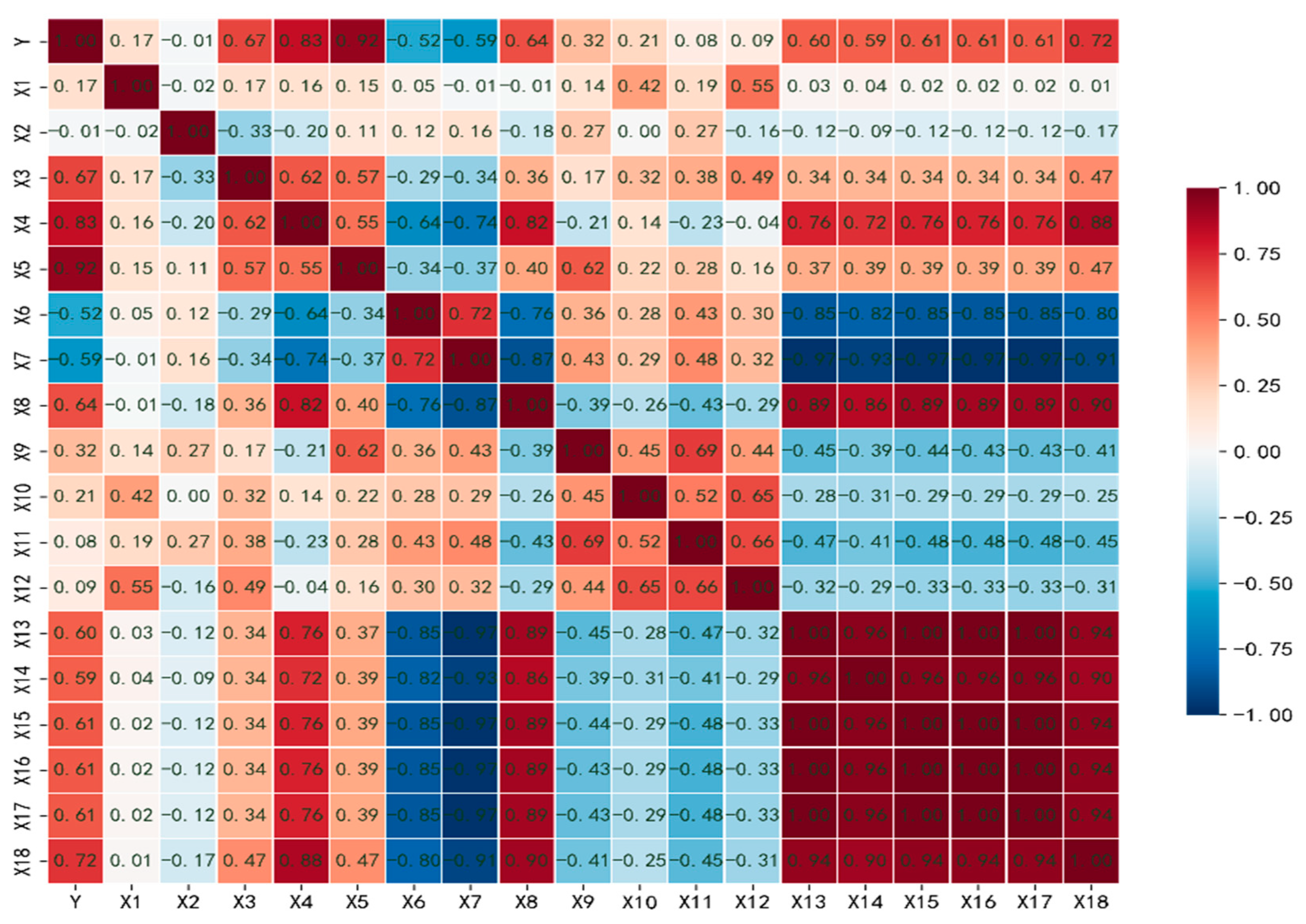
3.1. Correlation Analysis of Influencing Factors of Carbon Emissions

The measured data of an oilfield transfer station in Northeast China in 2022 was selected as the data set, and the data of the oil field transfer station system was cleaned. Identify abnormal data through box plots based on Jupyter in the Anaconda platform and use Python language programming to reconstruct missing data. According to the national and industry-standard monitoring methods for the production data of the oilfield transfer station system, 16 major carbon emission influencing factors are selected and used as input parameters of the prediction model. The source of carbon emission influencing factors is the measured data of the oil field transfer station in Northeast China in 2022, as shown in

Table 1. A description of the variables of the model.

Variable	Name	Definition	Unit
Y	Carbon emissions	The total CO2 emissions	tones
X1	Pressure difference	The difference in pressure between the two points	MPa
X2	Temperature difference	The difference between the temperature of the object	°C
X3	Daily infusion volume	The amount of crude oil transported per day	t
X4	Daily power consumption	Electricity is consumed daily	kW·h
X5	Daily air consumption	The amount of natural gas consumed per day	m3
X6	Density	A measure of mass within a specific volume	kg/m3
X7	Specific heat capacity	Indicates the ability of a substance to absorb heat or dissipate heat	kJ/(kg °C)
X8	Fuel calorific value	Indicates the amount of heat release capacity when the fuel is completely burned	GJ/ten thousands Nm3
X9	Thermal energy provided	Heat provided	kJ
X10	Pressure energy provided	Pressure energy provided by the outside world	kJ
X11	Oil absorbs heat energy	The thermal energy carried by the logistics entering the transfer station	kJ
X12	The pressure energy absorbed by the oil	Enter the transfer station logistics to carry pressure energy	kJ
X13	Thermal energy utilization	The efficiency with which heat energy is utilized	%
X14	Electrical energy utilization	The efficiency with which electrical energy is utilized	%
X15	Power consumption per unit of liquid volume collection and transmission	The power consumption of the transfer station system per 1t of produced liquid processed	kW·h/t
X16	Gas consumption per unit of liquid volume collection and transportation	The gas consumption of the transfer station system per 1t of produced liquid processed	m3/t
X17	Comprehensive energy consumption per unit of liquid volume	The comprehensive energy consumption of the transfer station system per 1t of produced liquid processed	kgce/t
X18	Transfer station energy utilization	The extent to which the energy of the transfer station system is used efficiently	%

.

Due to the different units of carbon emission influencing factors, the order of magnitude difference is large, so it is necessary to normalize the value into a number between [0, 1]; the purpose of normalization processing is to eliminate the order of magnitude difference between the data, to avoid large errors due to the large difference in the magnitude of the input data. This article adopts the following normalization method:

$$x_i^{*}=\frac{x_i-x_{\min }}{x_{\max }-x_{\min }}$$

(21)

where x_min is the minimum value in the influencing factor data series, x_max is the maximum value in the influencing factor data series, $x_i^{*}$ is the initial input data with the normalized data.

In the oil field transfer station system, there is a linear relationship between carbon emission and energy utilization rate. However, there is a linear relationship between carbon emissions and comprehensive energy consumption per unit of liquid volume. Pearson correlation coefficient can measure the wireless correlation between two features and the degree of correlation. Therefore, the Pearson correlation coefficient is used to measure the correlation between carbon emissions and other characteristics. The specific results are shown in Figure 4:

In the oil field transfer station system, there is a linear relationship between carbon emissions and energy utilization, and there is a linear relationship between carbon emissions and comprehensive energy consumption per unit of liquid quantity. The Pearson correlation coefficient can measure the wireless correlation between the two characteristics, so the Pearson correlation coefficient is used to measure the correlation between carbon emissions and other characteristics. The Pearson correlation coefficient was used to analyze the data of oilfield transfer stations, and the factors that had a greater impact on carbon emissions were found, and the energy utilization rate, comprehensive energy consumption per unit liquid volume, gas consumption per unit liquid volume, and power consumption per unit liquid volume were greatly affected. In order to avoid multicollinearity, X18 and X1–X12, which have great influence, are selected to model.

3.2. Example Application of Improved GA-Decision Tree (IGA-Decision Tree) Algorithm

In the given data sample, dividing the training, setting into K equal parts, taking out K − 1 parts for modeling, and using the remaining part of the sample to validate the established model, calculating the prediction error of this small part of the sample. Taking different training and testing sets each time and repeating the modeling K times, taking the average prediction error of K models as the final model error. Due to leaving a certain number of samples for validation during each modeling, the decision tree model based on K-fold cross-validation has stronger resistance to overfitting compared to the modeling method, where the entire training set participates in training. This article uses an Improved GA algorithm to optimize the three parameters of the decision tree: maximum number of splits, minimum number of leaf nodes, and minimum number of root nodes. It sets the upper and lower bounds of the optimization interval to [100, 1, 2] and [500, 5, 20], respectively, and sets the population number and maximum iteration times of the improved GA to 30 and 50. The improved GA algorithm and decision tree model are connected through fitness functions. The fitness function in this article should be the average cross-validation error rate, which can be calculated from Equations (22) and (23):

$$Fi{t}^{*}=\frac{1}{K}{\displaystyle {\sum }_{i=1}^{K}fi{t}_i}$$

(22)

$$fi{t}_i=\frac{1}{N}{{\displaystyle {\sum }_{q=1}^{N_{}}(y_q-y{\prime }_q)}}^2$$

(23)

where fit_i represents the cross-validation error of the ith fold and represents the predicted mse value of the validation fold; N is the number of samples per fold, y_q and y′_q represent the true and predicted values of the qth test sample in the validation compromise; Fit* represents the average cross-validation error, which is the final fitness function value.

After a finite number of iterations, the traversal scatter plot of the GA decision tree and the improved GA decision tree algorithm for searching for key hyperparameters is shown in Figure 5.

After a finite number of iterations, the traversal scatter plot of GA and improved GA for searching for key hyperparameters of the decision tree is shown in Figure 1. This is similar to the RF default parameter setting (default MinLeafSize = 1, MinParent = 10). When MinLeafSize and MinParent are small, the tree model has sufficient nodes to mine the data information in the training set. The model that improves the GA search for key hyperparameters performs better than the GA model. Further, the search–iteration curve under the optimal hyperparameter value is shown in Figure 6.

With the continuous advancement of the search process, the average cross-validation error continues to decrease, and the value of k is 4, and finally convergence is reached in the 35th generation.

4. Empirical Results and Discussion

The IGA-decision tree algorithm can combine the global optimization ability of the IGA-decision tree algorithm and the local search ability of the decision tree algorithm to solve the risk problem of the decision tree becoming stuck in the local optimal solution and improve its generalization and learning ability. Therefore, the IGA-decision tree algorithm can obtain output values faster than the decision tree, which is a clear advantage for involving large amounts of data.

In order to quantitatively analyze the effect of the optimized model, the performance of the IGA-decision tree and decision tree on the training set and testing set are plotted in Figure 7 and Figure 8, respectively.

As shown in Figure 7, the fitting effect of the IGA-decision tree with cross-validation and IGA-decision tree optimization on the training set is weaker than that of the decision tree because the fitness function during parameter tuning is the average cross-validation error rate. Each fold submodel is part of the training subset that does not participate in training, which reduces the goodness-of-fit in the training stage to a certain extent.

As shown in Figure 8, in the test set, the prediction error RMSE of the IGA-decision tree and GA-decision tree was 74.5181 and 228.4773, respectively, indicating that the IGA-decision tree has a better generalization performance in unknown sample sets.

In this paper, the IGA-decision tree algorithm is mainly used for its high accuracy and the effectiveness of predicted values. In order to further verify the feasibility and accuracy of IGA-decision tree model prediction, square correlation coefficient (R²) and mean absolute proportional error (MAPE) were used for evaluation. Evaluation indicators are defined as follows:

$$R^2=\frac{{\left[n{\displaystyle \sum {}_{i=1}^{n}f\left(x_i\right)y_i-{\displaystyle \sum {}_{i=1}^{n}f\left(x_i\right){\displaystyle \sum {}_{i=1}^n{y}_i}}}\right]}^2}{\left[n{\displaystyle \sum {}_{i=1}^n}f{\left(x_i\right)}^2-{\left({\displaystyle \sum {}_{i=1}^n}f\left(x_i\right)\right)}^2\right]\left[n{\displaystyle \sum {}_{i=1}^n}{y}_i{}^2-{\left({\displaystyle \sum {}_{i=1}^n}{y}_i\right)}^2\right]}$$

(24)

$$MAPE=\frac{1}{n}{\displaystyle \sum _{i=1}^n\frac{|Y_i-Y^{\wedge }{}_i|}{\left|Y_i\right|}}\times 100\%$$

(25)

where n is the number of samples; $Y_i$ is the actual value; and $Y^{\wedge }{}_i$ is the predicted value. R² is the degree to which the variance of the dependent variable can be explained by the independent variable, and the closer to one, the better the model effect; MAPE is the ratio of the absolute value of all sample errors compared to the actual value, and the closer the value is to 0, the more accurate the model; the data are cross-validated, and the optimal model prediction result error pair is shown in

Table 2. Results error comparison.

Predictive Models	RMSE	R2	MAPE/%
Decision tree	195.7539	0.86	8.02
GA-Decision tree	228.4773	0.97	3.35
IGA-Decision tree	74.5181	0.99	2.06

. R² was higher than that of the other two prediction models, indicating that the IGA-decision tree predictive model had a good and stable prediction effect.

When predicting carbon emissions for a specific oilfield transfer station, the IGA-decision tree model showed improvements compared to the GA-decision tree and decision tree models. The R² value increased by 0.02 and 0.13, respectively, while the RMSE value decreased by 153.9594 and 121.2358, respectively. In summary, although the IGA-decision tree sacrifices part of its fitting accuracy in the training phase, based on K-fold cross-validation, the trained model has a stronger adaptability to the test set. It has been shown that the proposed improvement strategy can effectively enhance the overfitting resistance of decision trees.

In the field of carbon emissions prediction, many traditional and classical forecasting methods have been widely used, including decision trees, support vector machines, and other single-model methods. The decision tree model has the advantage of being insensitive to missing values, can handle irrelevant feature data, and is easy to understand and implement. However, this algorithm is also easy to converge to a non-global local optimal solution; however, the generalization performance of such a model on the data is very poor, and the phenomenon of overfitting occurs. In contrast, the IGA-decision tree model is optimized on the basis of the decision tree model and searches for the optimal solution globally. The model has short prediction times, improved accuracy, and prevents overfitting.

5. Conclusions and Recommendations

(1)

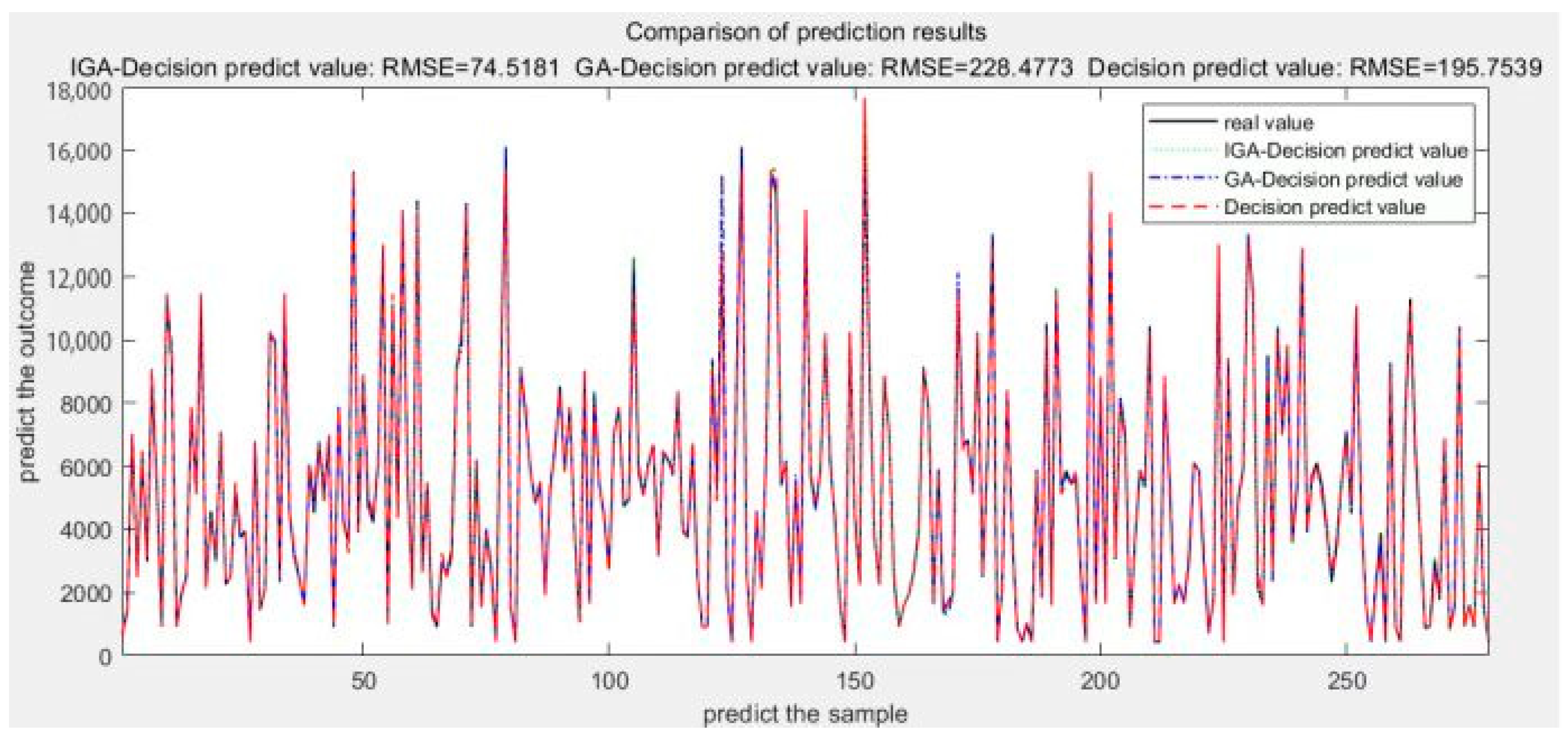
This paper proposes an improved GA-decision tree algorithm. It introduces chaotic mapping to initialize the population, aiming to achieve a uniform distribution of initial particles in the search space and increase population diversity. Additionally, a Firefly disturbance strategy was adopted to avoid the problem of genetic algorithms becoming trapped in local optima during the later stages of the search. The results show that this model can accurately predict the carbon emissions of the oilfield transfer station system, which verifies the accuracy and reliability of the model. When predicting carbon emissions for a specific oilfield transfer station, the IGA-decision tree model showed improvements compared to the GA-decision tree and decision tree model. The R² value increased by 0.02 and 0.13, respectively, while the RMSE value decreased by 153.9594 and 121.2358, respectively. It has high accuracy in predicting the carbon emissions of the oilfield transfer station system, which can provide an important basis for related work.

(2)

Under the “dual carbon” development strategy, the petroleum and petrochemical industry is facing carbon reduction challenges, especially the energy consumption and carbon emission problems faced by China’s oil and gas extraction industry. In this paper, taking an oilfield transfer station in Northeast China as an example, the carbon emissions of the transfer station were calculated using the IPCC method, and the IGA-decision tree model was used to search for optimization globally. The model validation results showed that this model had high accuracy and could be used to predict the carbon emissions of the oilfield transfer station system. This is of practical significance for carbon accounting, energy conservation, and carbon reduction and fills the research gap in carbon emission prediction in energy Internet projects.

(3)

The model also has some limitations: the study chose MAPE and R² as evaluation indicators but did not explain why these indicators were selected. At the same time, these evaluation indicators could only reflect part of the model performance, and other evaluation indicators might need to be considered to fully evaluate the accuracy and stability of the model. As the prediction interval expands, the predictive power of the model also decreases. Therefore, the above issues need to be improved in subsequent studies.

(4)

To further improve the accuracy and precision of carbon emissions prediction models in the future, it is recommended that more accurate and comprehensive data are collected while enhancing data availability. Additionally, exploring new machine learning algorithms, deep learning techniques, or employing ensemble modeling approaches could be beneficial in enhancing predictive performance. Performing sensitivity analysis on key factors in carbon emissions prediction models could help study the impact of different variables on prediction results. This could aid in identifying the main driving factors and provide a scientific basis for prioritizing emission reduction measures.

References

1. Wei, S.; Wang, T.; Li, Y. Influencing factors and prediction of carbon dioxide emissions using factor analysis and optimized least squares support vector machine. J. Environ. Eng. Res. 2017, 22, 175–185. [Google Scholar] [CrossRef]
2. Faruque, O.; Rabby, A.J.; Hossain, A.; Islam, R.; Rashid, M.U.; Muyeen, S. A comparative analysis to forecast carbon dioxide emissions. J. Energy Rep. 2022, 8, 8046–8060. [Google Scholar] [CrossRef]
3. Chen, W.J.; Wu, X.G.; Xiao, Z. Prediction of carbon emissions from road traffic in four major economic regions in China and assessment of emission reduction potential: Scenario model based on private car trajectory data. J. Econ. Geogr. 2022, 42, 44–52. [Google Scholar]
4. Xu, J.H.; Wang, K. Medium- and long-term carbon emission forecasting and technical emission reduction potential analysis of China’s civil aviation industry. J. Environ. Sci. China 2022, 42, 3412–3424. [Google Scholar]
5. Li, X.Y.; Zhao, R.J.; Gao, C.N.; Xie, X.L. Analysis of decoupling of carbon emissions from China’s civil aviation transport and peak forecasting. J. Environ. Pollut. Prev. 2022, 44, 729–733, 739. [Google Scholar]
6. Hu, J.B.; Zhao, K.; Yang, Y.H. Research on the prediction and control factors of China’s industrial carbon emission peaking: Empirical analysis based on BP-LSTM neural network model. J. Guizhou Soc. Sci. 2021, 9, 135–146. [Google Scholar]
7. Shi, D.; Li, P. Simulation of industrial carbon emission structure and policy impact under the “dual carbon” goal. J. Reform 2021, 12, 30–44. [Google Scholar]
8. Bian, Y.; Lin, X.Q.; Zhou, X.; Cui, W.J. Spatial-temporal evolution characteristics and influencing factors of industrial carbon emissions in Beijing-Tianjin-Hebei. J. Environ. Sci. Technol. 2021, 44, 37–47. [Google Scholar]
9. Liu, X.Z.; Yang, X. Variable Screening of Influencing Factors of China’s Carbon Emissions: Based on PLS-VIP Method. J. Environ. Ecol. 2019, 1, 60–65. [Google Scholar]
10. Wang, X.Y.; Zhou, S.M.; Xu, X.L.; Zhou, S.J. Analysis of influencing factors of carbon emission allowance price based on graph structure adaptive Lasso. J. Stat. Inf. Forum 2022, 37, 73–83. [Google Scholar]
11. Ke, H.; Zhang, X.S.; Cheng, Z.Z. Research on carbon emission prediction in Shanxi Province based on quadratic decomposition BAS-LSTM. J./OL. Oper. Manag. 2023, 1–14. [Google Scholar]
12. Gao, J.H.; Zheng, B.Z.; Zhou, W.H.; Li, P. Research on carbon emission prediction of urban transportation based on GA-SVR. J. East China Univ. Technol. (Nat. Sci. Ed.) 2022, 45, 269–274. [Google Scholar]
13. Hao, J.Y.; Gao, J. Based on NSGA-II the BP neural network is improved to predict the carbon emission reduction of buildings. J. Energy Effic. Build. 2016, 44, 122–124. [Google Scholar]
14. Sun, W.; Zhang, X. China’s carbon emission prediction based on QPSO-LSSVM algorithm. J. State Grid Inst. Technol. Newsp. 2017, 20, 20–25. [Google Scholar]
15. Yan, F.Y.; Liu, S.X.; Zhang, X.P. Research on land carbon emission prediction based on PCA-BP neural network. West. J. Hum. Settl. 2021, 36, 1–7. [Google Scholar]
16. Zhang, D.; Wang, T.T.; Zhi, J.H. Carbon emission prediction and eco-economic analysis of Shandong Province based on IPSO-BP neural network model. J. Ecol. Sci. 2022, 41, 149–158. [Google Scholar]
17. Zhou, W.; Zeng, B.; Wang, J.; Luo, X.; Liu, X. Forecasting Chinese carbon emissions using a novel grey rolling prediction model. J. Chaos Solitons Fractals 2021, 147, 110968. [Google Scholar] [CrossRef]
18. Yu, S.; Zheng, S.; Li, X. The achievement of the carbon emissions peak in China: The role of energy consumption structure optimization. J. Energy Econ. 2018, 74, 693–707. [Google Scholar] [CrossRef]
19. Yan, W.; Huang, Y.R.; Zhang, X.Y.; Gao, M.F. Carbon emission prediction of blue economic zone in Shandong Peninsula based on STIRPAT model. J. Univ. Jinan Nat. Sci. Ed. 2021, 35, 125–131. [Google Scholar]
20. Qu, P.; Liu, C.; Li, D.Z.; Guo, B.Q. Research on the development strategy of electric energy substitution under the goal of “carbon neutrality”. J. Electr. Demand Side Manag. 2021, 23, 1–3, 9. [Google Scholar]
21. Zhao, J.M. Incentive mechanism and realization method of transportation carbon emission reduction in megacities. J. Ecol. Econ. 2021, 37, 34–39. [Google Scholar]
22. Hu, M.F.; Zheng, Y.B.; Li, Y.H. Prediction of peak transportation carbon emissions in Hubei Province under multiple scenarios. J. Environ. Sci. 2022, 42, 464–472. [Google Scholar]
23. Xu, Y.G.; Song, W.X. Research on carbon emission prediction of construction industry based on FCS-SVM. J. Ecol. Econ. 2019, 35, 37–41. [Google Scholar]
24. Salman, B.; Ong, M.Y.; Nomanbhay, S.; Salema, A.A.; Sankaran, R.; Show, P.L. Thermal analysis of nigerian oil palm biomass with sachet-water plastic wastes for sustainable production of biofuel. Processes 2019, 7, 475. [Google Scholar] [CrossRef]
25. Hou, Y.; Iqbal, W.; Muhammad Shaikh, G.; Iqbal, N.; Ahmad Solangi, Y.; Fatima, A. Measuring energy effificiency and environmental performance: A case of South Asia. Processes 2019, 7, 325. [Google Scholar] [CrossRef]
26. Hsiao, W.L.; Hu, J.L.; Hsiao, C.; Chang, M.C. Energy effificiency of the Baltic Sea countries: An application of stochastic frontier analysis. Energies 2019, 12, 104. [Google Scholar] [CrossRef]
27. Paul, A.; Martins, L.M.; Karmakar, A.; Kuznetsov, M.L.; Novikov, A.S.; da Silva, M.F.C.G.; Pombeiro, A.J. Environmentally benign benzyl alcohol oxidation and C-C coupling catalysed by amide functionalized 3D Co(II) and Zn(II) metal organic frameworks. J. Catal. 2020, 385, 324–337. [Google Scholar] [CrossRef]
28. Alabdullah, M.A.; Gomez, A.R.; Vittenet, J.; Bendjeriou-Sedjerari, A.; Xu, W.; Abba, I.A.; Gascon, J. A Viewpoint on the Refinery of the Future: Catalyst and Process Challenges. J. ACS Catal. 2020, 10, 8131–8140. [Google Scholar] [CrossRef]
29. Alexander, N.; Maxim, K.; Bruno, R.; Armando, P.; Georgiy, S. Oxidation of olefins with H2O2 catalysed by salts of group III metals (Ga, In, Sc, Y and La): Epoxidation versus hydroperoxidation. J. Catal. Sci. Technol. 2016, 6, 1343–1356. [Google Scholar]
30. Al-Majidi, S.D.; Altai, H.D.S.; Lazim, M.H.; Al-Nussairi, M.K.; Abbod, M.F.; Al-Raweshidy, H.S. Al-Raweshidy, Bacterial Foraging Algorithm for a Neural Network Learning Improvement in an Automatic Generation Controller. J. Energ. 2023, 16, 2802. [Google Scholar]
31. Al-Majidi, S.D.; Kh AL-Nussairi, M.; Mohammed, A.J.; Dakhil, A.M.; Abbod, M.F.; Al-Raweshidy, H.S. Design of a Load Frequency Controller Based on an Optimal Neural Network. J. Energy 2022, 15, 6223. [Google Scholar]
32. Sun, W.; Liu, Y.D.; Li, M.Y.; Cheng, Q.L.; Zhao, L.X. Study on heat flow transfer characteristics and main influencing factors of waxy crude oil tank during storage heating process under dynamic thermal conditions. J. Energy 2023, 269, 127001. [Google Scholar] [CrossRef]
33. Lin, L.; Li, Y.M.; Wang, W. Energy-saving Management Measures in Oilfield Engineering Construction Processes. J. Stand. Qual. Chin. Pet. Chem. Ind. 2013, 33, 228. [Google Scholar]
34. Cheng, Q.L.; Liu, H.G.; Meng, L.; Wang, X.; Sun, W. Analysis and optimization of carbon emission from natural gas ethanolamine desulfurization process. J. Contemp. Chem. Ind. 2023, 52, 1389–1395. [Google Scholar]
35. Friedman, J.H. Greedy function approximation: A gradient boosting machine. J. Ann. Stat. 2001, 29, 1189–1232. [Google Scholar] [CrossRef]
36. Ahang, Y.; Wang, J.; Wang, X.; Xue, Y.; Song, J. Efficient selection on spatial modulation antennas: Learning or boosting. J. IEEE Wirel. Commun. Lett. 2020, 9, 1249–1252. [Google Scholar]
37. Liu, L.; Jiang, B.W.; Zhou, H.Y.; Pu, C.W.; Qian, P.F.; Liu, B. A Novel Particle Swarm Optimization Algorithm with Improved Sine Chaotic Mapping Integration. J. Xi’an Jiaotong Univ. 2023, 57, 183–191. [Google Scholar]
Figure 1. Genetic algorithm optimization decision tree grid search flowchart.
Processes 11 02738 g001
Figure 2. Comparison of Tent and Chebychev maps. (a) Tent. (b) Chebyshev.
Processes 11 02738 g002
Figure 3. Main training flowchart for improving GA decision tree algorithm.
Processes 11 02738 g003
Figure 4. Correlation analysis of influencing factors.
Processes 11 02738 g004
Figure 5. The traversal scatterplot of key hyperparameter. (a) GA-Decision Tree Model. (b) IGA-Decision Tree Model.
Processes 11 02738 g005
Figure 6. The genetic–iteration curve.
Processes 11 02738 g006
Figure 7. The training set predicts the outcome.
Processes 11 02738 g007
Figure 8. The testing set predicts the outcome.
Processes 11 02738 g008