A Low-Carbon Scheduling Method of Flexible Manufacturing and Crane Transportation Considering Multi-State Collaborative Configuration Based on Hybrid Differential Evolution

Abstract

With increasingly stringent carbon policies, the development of traditional heavy industries with high carbon emissions has been greatly restricted. Manufacturing companies surveyed use multifunctional machining machines and variable speed cranes, as the lack of rational planning results in high energy wastage and low productivity. Reasonable scheduling optimization is an effective way to reduce carbon emissions, which motivates us to work on this research. To reduce the comprehensive energy consumption of the machining process and transportation process in an actual manufacturing environment, this paper addresses a new low-carbon scheduling problem of flexible manufacturing and crane transportation considering multi-state collaborative configuration (LSP-FM&CT-MCC). First, an integrated energy consumption model based on multi-state machining machines and cranes is established to optimize the overall energy efficiency of the production process. Then, a new hybrid differential evolution algorithm and firefly algorithm with collaborative state optimization strategy (DE-FA-CSOS) is proposed to solve the proposed MIP model. In DE-FA-CSOS, the differential evolution algorithm (DE) is used for global search, and the firefly algorithm (FA) is used for local search. The collaborative state optimization strategy (CSOS) is proposed to guide the search direction of the DE-FA algorithm, which greatly improves the performance of the hybrid algorithm. Finally, the practicality and superiority of the solution method are verified by examples. The results show that machining and transportation energy consumption is reduced by 25.17% and 34.52%, respectively. In the context of traditional optimization methods and manual scheduling modes facing failure, the method has a broad application background for manufacturing process optimization in such workshops, which is of guiding significance for promoting the low-carbon development of traditional heavy industry manufacturing.

1. Introduction

The increasing carbon emissions have caused a series of environmental pollution problems, and the global manufacturing industry urgently needs to transition to low carbon. According to relevant surveys, the energy efficiency of the manufacturing industry is low and pollution emissions are high in China, e.g., the proportion of industrial GDP, 33.2%, is obtained by consuming 70% of the national energy in 2022. With coal and oil accounting for 56% and 18.5%, respectively, of China’s energy mix in 2022, these two high-carbon emissions fuels remain the country’s main energy sources [1]. In this context, the government has introduced a series of strict countermeasures to accelerate the industrial transformation to low-carbon, which has greatly restricted the development of high-emission traditional heavy manufacturing industry [2]. It is well known that energy consumption is the primary source of carbon emissions. According to the National Bureau of Statistics, China’s power sector emitted about 9.64 billion tons of carbon dioxide in 2019, accounting for 45.8% of the country’s total emissions. The power sector has been the industry that generates the most carbon emissions in China, causing serious environmental problems [3]. So, improving energy efficiency can effectively reduce carbon emissions in manufacturing industries. In traditional heavy industry manufacturing enterprises, the machining process is the main contributor to carbon emissions. In addition, the energy consumption during the transportation of large workpieces cannot be ignored, and the proportion of transportation energy consumption in the actual manufacturing process of the surveyed enterprises can reach 38% [4]. Through the collaborative scheduling optimization of the machining process and the transportation process, the machining energy consumption and transportation energy consumption of the production process can be effectively reduced, thus reducing carbon emissions. Therefore, it is of great significance to study the problem of low-carbon coordination scheduling.

In the production environment of heavy manufacturing enterprises, the machining process and the transportation process in the workshop are often interrelated and affect each other. This makes the production process prone to problems such as idle machines and chaotic planning, making scheduling much more difficult. In addition, due to the increasing complexity of the production process, the use of variable-speed multi-functional machining machines and cranes is the development trend of the heavy manufacturing industry. This type of equipment has a variety of states, such as on/off and changing speed during operation. Changes in the various operating states of machines and cranes directly affect the entire production process, further increasing the flexibility and complexity of the manufacturing environment. However, various existing manufacturing systems in traditional heavy industries still rely heavily on manual scheduling. Limited by human decision-making, this mode cannot cope with such a complex production environment. It leads to the disorganized production process in heavy manufacturing enterprises, resulting in serious energy waste. Therefore, it is urgent to design an effective optimization method to optimize the multi-state collaborative configuration of the machining process and the transportation process to improve the energy efficiency of the manufacturing system and reduce the carbon emissions of the production process of heavy manufacturing enterprises.

On this basis, this paper introduces a new low-carbon scheduling problem of flexible manufacturing and crane transportation considering multi-state collaborative configuration (LSP-FM&CT-MCC) based on the background of a large cement equipment manufacturing company. The contributions of this paper are summarized as follows: (1) A new mixed integer programming (MIP) model is established to solve LSP-FM&CT-MCC. The model describes in detail the energy consumption of machines and cranes in various states. The goal of the model is to minimize the total energy consumption and makespan; (2) A novel hybrid differential evolution (DE) with firefly algorithm (FA) and collaborative state optimization strategy (CSOS) is developed to solve the model. The CSOS consists of a load transport state optimization strategy and a machining state optimization strategy (This strategy is used to configure the state of machines and cranes to save energy, mainly by shutting down equipment and reducing operating speeds).

The remainder of this paper is organized as follows. Section 2 reviews and summarizes the relevant literature. Section 3 describes the problems. Next, the framework and detailed components of the hybrid DE-FA-CSOS algorithm are presented in Section 4. To demonstrate the effectiveness and superiority of the algorithm, Section 5 illustrates a case study. The experimental results are discussed in Section 6. Finally, the conclusions and further research prospects for this problem are presented in Section 7.

2. Literature Review

This section reviews relevant studies on low-carbon manufacturing scheduling optimization and manufacturing scheduling optimization considering transportation.

2.1. Low-Carbon Manufacturing Scheduling Optimization

Research on low-carbon manufacturing scheduling problems in various manufacturing environments can be divided into two main categories: flow shop scheduling problems and job shop scheduling problems.

For the optimization of low carbon flow shop scheduling, the construction of optimization models and algorithm innovation are the research focus of scholars. Tirkolaee et al. [5] proposed a novel dual-objective mixed-integer linear programming model with outsourcing options and just-in-time delivery to simultaneously minimize the total cost and total energy consumption of the production system. Yu and Han [6] examined machine scheduling problems inspired by the semiconductor manufacturing production environment and developed a flow shop scheduling model focusing on an important special case with proportional processing times. Fu et al. [7] proposed a dual-objective stochastic hybrid flow shop deteriorating scheduling problem to minimize makespan and total tardiness. For scheduling problems of energy-efficient block flow shop with setup time, Han et al. [8] constructed a multi-objective optimization model with makespan and energy consumption criteria. Shao et al. [9] developed a MIP model that considers time-of-use electricity tariffs for the distributed heterogeneous mixed-flow store scheduling problem under unequal time tariffs.

Furthermore, some scholars contributed algorithmic improvements and innovations to improve the optimization effect. For the distributed permutation flow shop with sequence-dependent setup times scheduling problem, Huang et al. [10] proposed three constructive heuristics and an effective discrete artificial bee colony algorithm. For the distributed heterogeneous hybrid flow shop scheduling problem with unrelated parallel machines and the sequence-dependent setup time, Li et al. [11] proposed an improved artificial bee colony algorithm. Wu et al. [12] focused on the robotic cell scheduling problem with batch-processing machines, and a green schedule algorithm and a multi-objective differential evolution algorithm are proposed to optimize the makespan and energy consumption of the batch-processing machines simultaneously. Pan et al. [13] executed five meta-heuristics are executed to solve the distributed batch flow alignment process shop scheduling problem. Qin et al. [14] considered the limited waiting time between batch and discrete processors to develop a learning-based scheduling method through custom genetic programming.

Research on low-carbon scheduling optimization in job shop scheduling is divided into two groups: machining process optimization and comprehensive method application.

For the machining process optimization group, Afsar et al. [15] established a multi-objective optimization model based on the green job shop scheduling problem with uncertain processing times, in which the dual goal is to minimize energy consumption and total manufacturing span during machine idle time. Wei et al. [16] proposed an energy-aware estimation model to compute different energy consumptions for different operating conditions of a machine. Duan et al. [17] developed a dynamic scheduling mathematical model considering machine idle time schedule and speed level selection during processing and proposed a method of calculating machine energy consumption and completion time under different states. Wu et al. [18] established a multi-objective mathematical model with the joint minimum of maximum completion time and total setup time, which effectively reduces the fixture loading and unloading time. Luo et al. [19] developed a hierarchical multi-intelligence deep reinforcement learning-based real-time scheduling approach to address the dynamic scheduling problem with new job insertions and machine breakdown. Jiang et al. [20] introduced a resilient scheduling model for the steel mill by considering the buffering times and machining speeds to enable the solution to absorb random disturbances and recover quickly.

For the comprehensive method application, Feng et al. [21] proposed an integrated method for intelligent green scheduling of the sustainable flexible workshop with edge computing considering uncertain machine state. He et al. [22] proposed a multi-objective optimization framework based on the fitness evaluation mechanism and an adaptive local search strategy. Wang et al. [23] presented a multi-period production planning-based real-time scheduling approach to carry out real-time scheduling based on real-time manufacturing data. Based on the processing energy characteristics in resource-constrained processing environments, Li et al. [24] proposed a comprehensive solution to minimize the energy consumption and completion time of resource-constrained. Kovalenko et al. [25] proposed a multi-intelligent control strategy to improve the flexibility of manufacturing systems. Kung and Liao [26] consider the optimization of joint predictive maintenance and job scheduling problems to minimize total shortage losses and develop a heuristic algorithm based on the Tabu search.

Extensive studies have been conducted on the scheduling problem of manufacturing systems with different influencing factors (including factors such as processing speed, setup, and time-sharing tariff). However, there is no further study on the multi-state collaborative configuration optimization problem. It is worth noting that machine and crane multi-states often interact with each other, further increasing the complexity of the optimization problems.

2.2. Manufacturing Scheduling Optimization Considering Transportation

For the flow shop scheduling optimization problem considering transportation, Wang et al. [27] considered constraints such as transportation capacity and transportation time and proposed a heuristic optimization algorithm. Lei et al. [28] studied the flexible flow shop scheduling problem with dynamic transportation waiting times and developed a memetic algorithm integrated with the waiting time calculation approach. For the permutation flow shop scheduling problem with sequence-dependent setup time, Xin et al. [29] designed an improved discrete whale swarm optimization algorithm that combines differential evolution, augmented search, and job-swapped mutation to enhance performance; Yuan et al. [30] considered both sequence-dependent setup time between groups and the transportation time between machines and proposed a novel discrete differential evolution mechanism with a cooperative-oriented optimization strategy to evolve both the sequence of jobs in each group and the sequence of groups synergistically.

For the job shop scheduling optimization problems considering transportation, Goli et al. [31] investigated the role of AGVs and human factors in cell formation and scheduling of parts under fuzzy processing time and developed a hybrid genetic algorithm and a whale optimization algorithm. Zhou et al. [32] focused on the green scheduling problem of the flexible manufacturing cell with material handling robots and proposed a levy flight and weighted distance-updated multi-objective grey wolf algorithm. Ren et al. [33] considered the constraints of transportation resources and transportation time, and a novel particle swarm optimization algorithm integrated with genetic operators is developed to respond to dynamic events and generate the rescheduled plan in time. Li et al. [34] proposed an efficient hybrid of iterated greedy and simulated annealing algorithms, taking into account the two objectives of makespan and total energy consumption. Li and Lei [35] studied the energy-efficient flexible job shop integrated scheduling problem considering transportation and process-dependent setup times and developed an imperialist competitive algorithm with feedback to minimize the makespan, total tardiness, and total energy consumption, simultaneously.

For other forms of job shop scheduling optimization considering transportation, Zhao et al. [36] proposed a digital twin-driven energy-efficient multi-crane scheduling and crane number selection method for multi-crane systems. Sun et al. [37] proposed two novel robotic job-shop scheduling models with robot movement and deadlock considerations to avoid transportation conflicts for the deadlock problem of robot-driven production lines. Numerical examples illustrate that models can completely avoid transportation conflicts. Zou et al. [38] studied a novel automatic guided vehicle (AGV) energy-efficient scheduling problem with release time and established a multi-objective mathematical model with energy consumption, number of AGVs used, and customer satisfaction as optimization objectives, and proposed an efficient multi-objective greedy algorithm. Li et al. [39] used deep reinforcement learning to address the dynamic flexible job shop scheduling problem with insufficient transportation resources. Zhao et al. [40] developed a model for the scheduling problem of considering multiple cranes and their dual-load capacity and proposed a heuristic method based on the two-stage model.

From the above studies, it is shown that a great deal of effort has been made to solve the scheduling problems of flow shops and job shops in different environments. However, while considering the optimization of transport energy consumption, most studies have yet to study the optimization problem of multi-state collaborative configuration of machines and cranes accordingly. To address the above limitations, this paper investigates a flexible manufacturing system with a crane transportation problem considering a multi-state collaborative configuration.

3. Formulation

In this section, the LSP-FM&CT-MCC is introduced in detail to the actual manufacturing environment of heavy equipment manufacturing enterprises. The corresponding MIP model considered comprehensive energy consumption and makespan was established. All symbol definitions in the text are set out in Nomenclature.

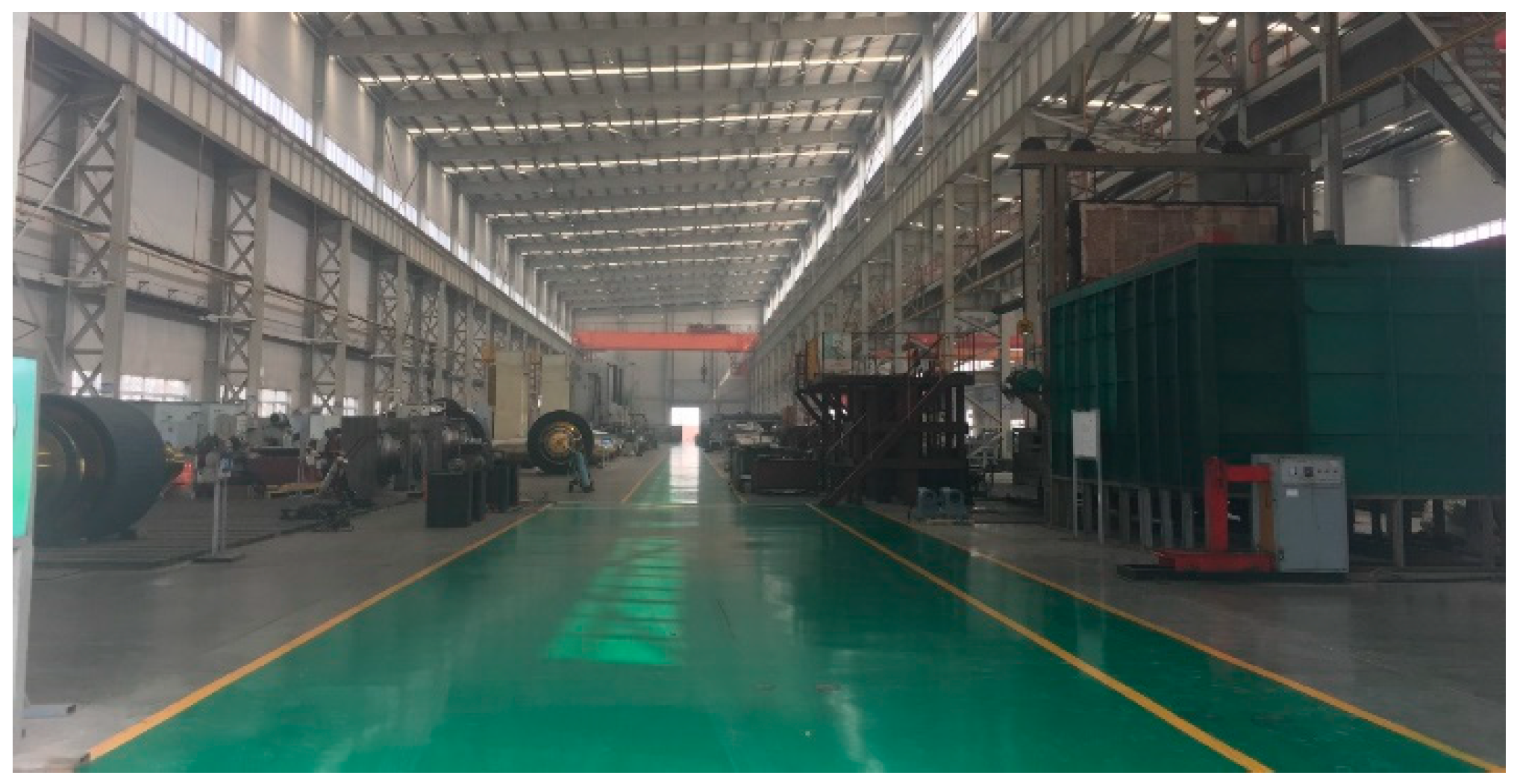
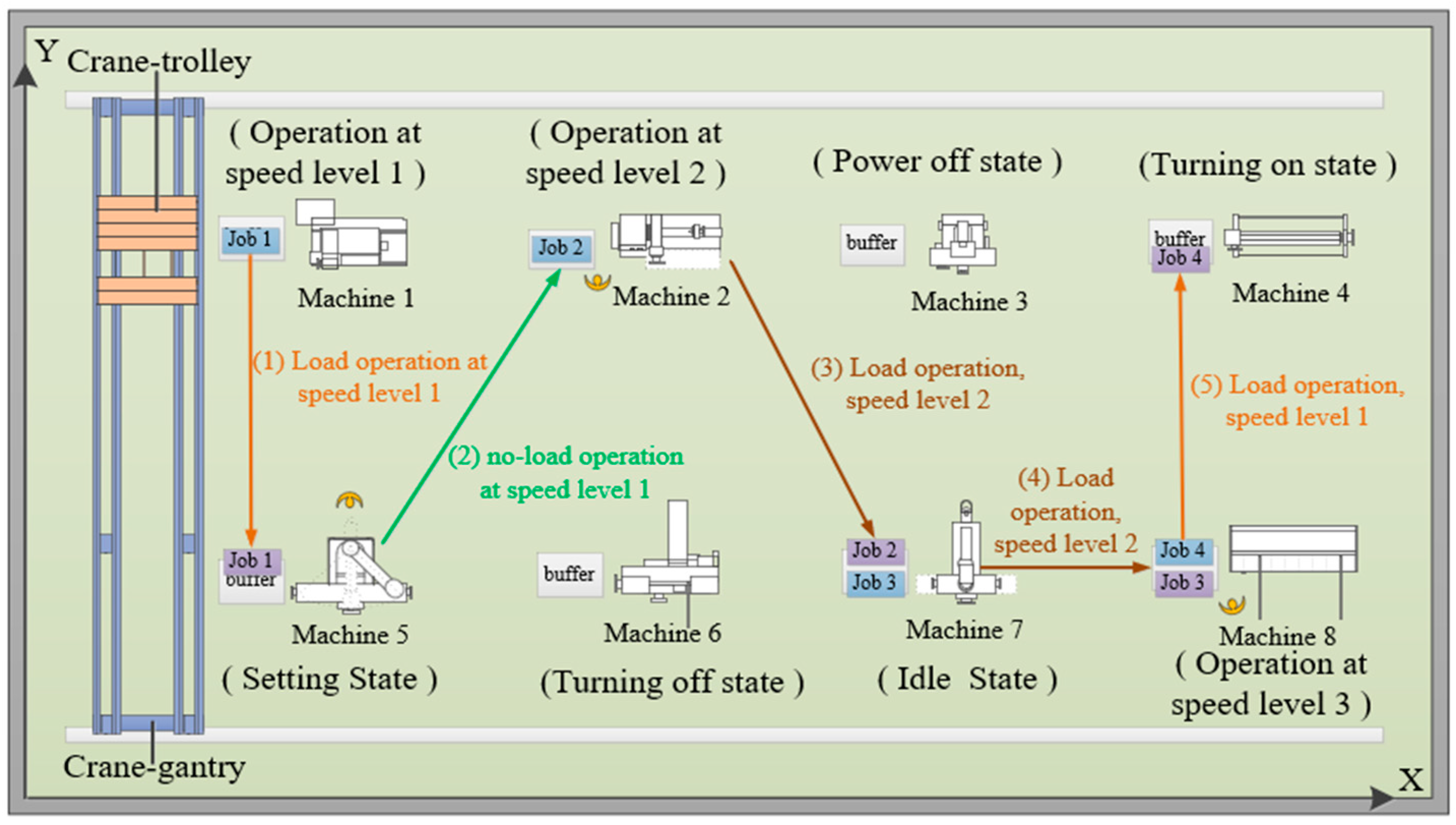
3.1. Problem Description

Figure 1 shows the actual workshop environment of the investigated company. The machining environment is a flexible manufacturing environment with multi-functional and multi-state machines. The transport equipment is a bridge crane located on the top of the workshop. The position of each machine is fixed and represented in the plane coordinate (X, Y). The crane consists of a gantry and a trolley. The gantry can only move in the X-axis direction and the trolley can only move in the Y-axis direction. Due to the discontinuity of workpiece processing, there are different states of the machining machine and crane, such as variable speed, on and off, and idle. In addition, the machining machine needs to go through the setting state before the speed changes. Therefore, the main scheduling tasks of the manufacturing system include the following three points: (1) Arrange the appropriate machining sequence of the workpiece; (2) Plan the path of the crane to transport the workpieces; (3) Collaborative configuration of the operating status of the machines and the crane. This paper considers two objectives: minimizing the total comprehensive energy consumption and makespan.

To illustrate the operation process of the workshop, a scheduling scheme shown in Figure 2 is taken as an example to describe: (1) First, the crane is in the power-off state above machine 1, which processes workpiece 1 at speed level 1. When workpiece 1 finishes processing on machine 1, the crane opens and transports workpiece 1 to machine 5. Machine 5 converts the processing speed of workpiece 1 by setting; (2) Second, the crane runs to the buffer area of machine 2 without loading and waits until workpiece 2 finishes processing. Meanwhile, to reduce the crane waiting time, machine 2 is processed at speed level 2; (3) Third, the crane delivers workpiece 2 to machine 7, unloads workpiece 2, loads workpiece 3, and waits in the loaded state until workpiece 4 finishing processing on machine 8. Simultaneously, machine 7 has already finished machining workpiece 3 and is in an idle state; (4) To shorten the crane load idle time, machine 8 is operated at speed level 3. After workpiece 4 is processed, the crane immediately transports workpiece 3 to machine 8; (5) Finally, the crane transports workpiece 4 to machine 4 and enters the power-off state above machine 4. Machine 4 enters the power-on state after receiving workpiece 4. In addition, machine 3 is turned off state to save energy consumption.

3.2. Assumptions

• Each workpiece can only be processed on one of the available machines with a certain speed at a certain time.
• Each machine can only process one workpiece at a certain time.
• The crane can only transport one workpiece at a certain time.
• The gantry and trolley cannot run at the same time for safety.
• The workpiece does not occupy the current machine after completing a certain process.
• When a certain process is completed, the transportation must be started after the next machine is idle for safety; otherwise, the crane needs to wait in place.

3.3. The Comprehensive Energy Consumption Model

In this section, to better analyze the energy consumption of machining and transportation processes, a comprehensive energy consumption model based on multiple states of machines and cranes is established. The comprehensive energy consumption is divided into two categories: machine processing process and crane transportation process. The comments of relevant notations are described in Nomenclature.

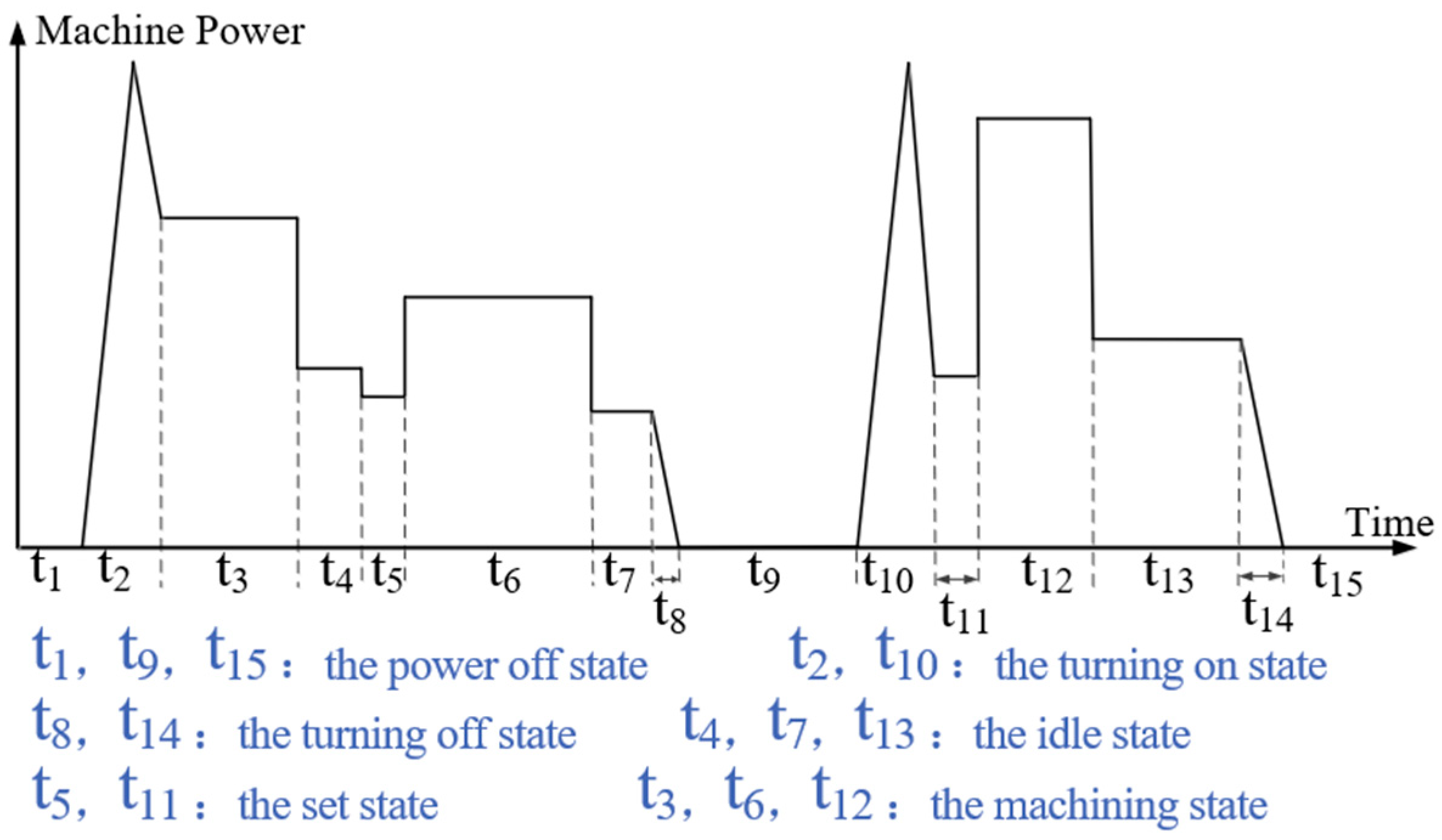
3.3.1. The Energy Consumption of the Machine Operation Process

In LSP-FM&CT-MCC, the input power of the machine changes with its state. There are four states for machines in total: the turning-on/off state, the idle state, the machining state, the power-off state, and the set state. Each machine has diverse kinds of speed levels, with different speed levels corresponding to different machining power and times. The machine is in an idle state between two adjacent tasks. There is an option to turn off the machine to save energy in idle time [41]. Turning on and off the machine need consumes a certain amount of energy. In particular, the machine needs to be set up first when switching between different speeds. To visualize the characteristics of the machine more, Figure 3 shows the variation of the machine’s power relative to the state in a real case.

• The energy consumption of the set state of the machine.

The amount of setting power is only related to the properties of the machine. The set energy consumption may be calculated by (1) and (2).

$$E^{ms}\left(P_{i,n}\right)=\left\{\begin{array}{l}{\displaystyle \sum _{m=1}^M{\displaystyle \sum _{q=1}^Q{P}_m^s\cdot T_{i,n,m,q}^s\cdot x_{i,n,m,q}}} , P_{i,n}\in \phi \left(P_{1,m}\right)\\ {\displaystyle \sum _{m=1}^M{\displaystyle \sum _{q=1}^Q{\displaystyle \sum _{i1=1}^{P_{i1}}{\displaystyle \sum _{n1}^{N}u\left(m,P_{i1,n1},P_{i,n}\right)\cdot v\left(Q_{i1,n1,m},Q_{i,n,m}\right)\cdot P_m^s\cdot T_{i,n,m,q}^s\cdot x_{i,n,m,q}}} , \mathrm{other}}}\end{array}\right.$$

(1)

$$E^{ms}={\displaystyle \sum _{n=1}^N{\displaystyle \sum _{i=1}^{P_n}{E}^{ms}\left(P_{i,n}\right)}}.$$

(2)

II.

The energy consumption of the machining state.

The processing energy consumption can be calculated with (3) and (4).

$$E^{mo}\left(P_{i,n}\right)={\displaystyle \sum _{m=1}^M{\displaystyle \sum _{q=1}^Q{P}_{m,q}^o\cdot T_{i,n,m,q}^o\cdot x_{i,n,m,q}}},$$

(3)

$$E^{mo}={\displaystyle \sum _{n=1}^N{\displaystyle \sum _{i=1}^{P_n}{E}^{mo}\left(P_{i,n}\right)}}.$$

(4)

III.

The energy consumption of idle state

The idle time of process P_i,n is calculated by (5). The idle energy consumption of the machine can be expressed by (6) and (7). In particular, the idle power changes with the machining speed level.

$$T_{i,n,m}^i=\left\{\begin{array}{l}0 , P_{i,n}\in \phi \left(P_{1,m}\right)\\ T{s}_{i,n}-{\displaystyle \sum _{q=1}^Q{\displaystyle \sum _{i1=1}^{P_{i1}}{\displaystyle \sum _{n1}^N{T}_{i,n,m,q}^s\cdot u\left(m,P_{i1,n1},P_{i,n}\right)\cdot v\left(Q_{i1,n1,m},Q_{i,n,m}\right)\cdot x_{i,n,m,q}}}}-{\displaystyle \sum _{i1=1}^{P_{i1}}{\displaystyle \sum _{n1=1}^{N}T{c}_{i1,n1}\cdot u\left(m,P_{i1,n1},P_{i,n}\right)}} , \mathrm{other}\end{array}\right.$$

(5)

$$E^{mi}\left(P_{i,n}\right)=\left\{\begin{array}{l}0 , P_{i,n}\in \phi \left(P_{1,m}\right)\cup y_{i,n,m}=1\\ {\displaystyle \sum _{m=1}^M{\displaystyle \sum _{q=1}^Q{P}_{m,q}^i\cdot T_{i,n,m}^i\cdot x_{i,n,m,q} , \mathrm{other}}}\end{array}\right.$$

(6)

$$E^{mi}={\displaystyle \sum _{n=1}^N{\displaystyle \sum _{i=1}^{P_n}{E}^{mi}\left(P_{i,n}\right)}}.$$

(7)

IV.

The energy consumption of turn-on/off state.

In scheduling, the turning-on/off energy consumption of the machine is related to the time of on and off. The total turning-on/off energy consumption of the production process is calculated by (8) and (9).

$$E^{mof}\left(P_{i,n}\right)={\displaystyle \sum _{m=1}^M{E}_m^{of}\cdot y_{i,n,m}},$$

(8)

$$E^{mof}={\displaystyle \sum _{n=1}^N{\displaystyle \sum _{i=1}^{P_n}{E}^{mof}\left(P_{i,n}\right)}}.$$

(9)

V.

The total energy consumption of the machine operation process.

The total energy consumption of the machining process is the sum of the above four components, expressed as (10).

$$E^m=E^{ms}+E^{mo}+E^{mi}+E^{mof}$$

(10)

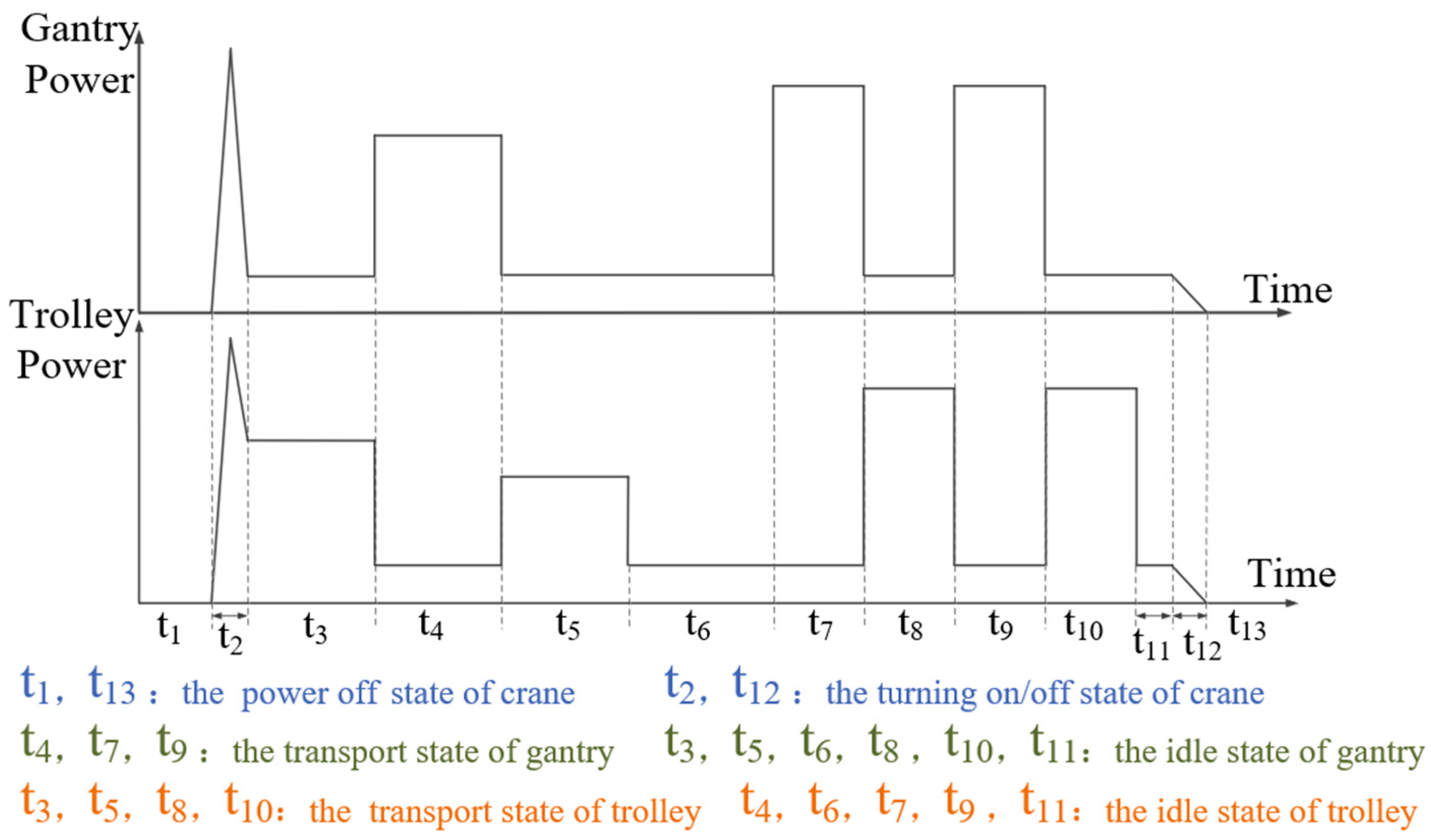
3.3.2. The Energy Consumption of Crane Operation Process

This section describes the crane operation process with a scheduling case in Figure 2. The corresponding schematic diagram of the crane power variation with the state is shown schematically in Figure 4, where the time for loading and unloading the workpiece is not considered. The states of the crane can be summarized into the following three: variable speed transport state, turning on/off state, and idle state. In particular, the crane does not need to be set for variable speed.

• The energy consumption of the crane idle state.

The idle phase of the crane is divided into two situations: load idle and no-load idle. The no-load idle time of the crane is calculated by (11), and the idle load time of the crane is calculated by (12). The energy consumption of unloaded idle and loaded idle is expressed by (13) and (14), respectively.

In particular, all workpieces do not need to be transported in the first process, so the corresponding idle time and energy consumption are zero.

$$T_{i,n}^{ni}=\left\{\begin{array}{l}0 , P_{i,n}\in \sigma \left(P_{1,n}\right)\cup P_{i,n}\in \phi \left(P_{1,m}\right)\\ {\displaystyle \sum _{i1=1}^{P_{n1}}{\displaystyle \sum _{n1=1}^N\max \left(T{c}_{i-1,n}-T{s}_{i1,n1}-T_{i,n}^{no,g}-T_{i,n}^{no,t},0\right)\cdot u\left(P_{i1,n1},P_{i,n}\right)}} , \mathrm{other}\end{array}\right.$$

(11)

$$T_{i,n}^{li}=\left\{\begin{array}{l}0 , P_{i,n}\in \sigma \left(P_{1,n}\right)\cup P_{i,n}\in \phi \left(P_{1,m}\right)\\ {\displaystyle \sum _{i2=1}^{P_{n2}}{\displaystyle \sum _{n2=1}^N{\displaystyle \sum _{m=1}^M{\displaystyle \sum _{q=1}^Q\max \left(T{c}_{i2,n2}-T{c}_{i-1,n},0\right)\cdot u\left(m,P_{i2,n2},P_{i,n}\right)\cdot x_{i,n,m,q}}}}} , \mathrm{other}\end{array}\right.$$

(12)

$$E^{ci}\left(P_{i,n}\right)=\left\{\begin{array}{l}0 , P_{i,n}\in \sigma \left(P_{1,n}\right)\cup P_{i,n}\in \phi \left(P_{1,m}\right)\cup \left(w_{i,n}^{ni}=1\cap w_{i,n}^{li}=1\right)\\ T_{i,n}^{ni}\cdot P_c^s , P_{i,n}\notin \sigma \left(P_{1,n}\right)\cap P_{i,n}\notin \phi \left(P_{1,m}\right)\cap \left(w_{i,n}^{ni}=0\cap w_{i,n}^{li}=1\right)\\ T_{i,n}^{li}\cdot P_c^s , P_{i,n}\notin \sigma \left(P_{1,n}\right)\cap P_{i,n}\notin \phi \left(P_{1,m}\right)\cap \left(w_{i,n}^{ni}=1\cap w_{i,n}^{li}=0\right)\\ \left(T_{i,n}^{ni}+T_{i,n}^{li}\right)\cdot P_c^s , P_{i,n}\notin \sigma \left(P_{1,n}\right)\cap P_{i,n}\notin \phi \left(P_{1,m}\right)\cap \left(w_{i,n}^{ni}=0\cap w_{i,n}^{li}=0\right)\end{array}\right.,$$

(13)

$$E^{ci}={\displaystyle \sum _{i=1}^{P_n}{\displaystyle \sum _{n=1}^N{E}^{ci}\left(P_{i,n}\right)}}.$$

(14)

II.

The energy consumption of crane turning on/off state.

There is an option to turn it off to save energy if the crane is idle for a long time. The crane turning on and off will generate energy consumption, and the size of the energy consumption is related to the number of times the crane is turned on and off. The energy consumption of the crane turning on/off is calculated by (15) and (16).

$$E^{cof}\left(P_{i,n}\right)=\left\{\begin{array}{l}0 , w_{i,n}^{ni}=w_{i,n}^{li}=0\\ \left(w_{i,n}^{ni}+w_{i,n}^{li}\right)\cdot E_c^{of} , w_{i,n}^{ni}\ne w_{i,n}^{li}\\ w_{i,n}^{ni}\cdot w_{i,n}^{li}\cdot E_c^{of} , w_{i,n}^{ni}=w_{i,n}^{li}=1\end{array}\right.,$$

(15)

$$E^{cof}={\displaystyle \sum _{n=1}^N{\displaystyle \sum _{i=1}^{P_n}{E}^{mof}\left(P_{i,n}\right)}}.$$

(16)

III.

The energy consumption of crane operation state.

During the operation of the crane, it is divided into two situations: load operation and no-load operation. The crane sometimes needs no-load transport to a designated machine to pick up a workpiece. After the workpiece is picked up, the crane transports it to the target machine. Therefore, the energy consumption corresponding to the above two cases will be generated during the operation process of the crane.

In the transport task of a process P_i,n, the no-load operation time of the gantry and the trolley are calculated by (17) and (18), respectively. Then, calculate the energy consumption of the crane no-load operation for P_i,n by (19). The load operation time of the gantry and trolley are calculated by (20) and (21), respectively. Equation (22) represents the energy consumption generated by the crane to complete the transport task of a process P_i,n. The energy consumption of the operation of the crane is the sum of the crane’s no-load operation energy consumption and load operation energy consumption, as shown in (23).

In particular, the crane has multiple operating speed classes, with different operating speeds corresponding to different operating powers and operating times, resulting in different energy consumption.

$$T_{i,n}^{no,g}={\displaystyle \sum _{i1=1}^{P_{n1}}{\displaystyle \sum _{n1=1}^N{\displaystyle \sum _{m=1}^M{\displaystyle \sum _{m1=1}^M{\displaystyle \sum _{q=1}^Q{\displaystyle \sum _{q1=1}^Q{\displaystyle \sum _{r=1}^R\left(\frac{\left|D{x}_m-D{x}_{m1}\right|\cdot z_{i,n,r}}{V_{g,r}}\right)\cdot u\left(P_{i1,n1},P_{i,n}\right)\cdot x_{i1,n1,m1,q1}\cdot x_{i-1,n,m,q}}}}}}}}$$

(17)

$$T_{i,n}^{no,t}={\displaystyle \sum _{i1=1}^{P_{n1}}{\displaystyle \sum _{n1=1}^N{\displaystyle \sum _{m=1}^M{\displaystyle \sum _{m1=1}^M{\displaystyle \sum _{q=1}^Q{\displaystyle \sum _{q1=1}^Q{\displaystyle \sum _{r=1}^R\left(\frac{\left|D{y}_m-D{y}_{m1}\right|\cdot z_{i,n,r}}{V_{t,r}}\right)\cdot u\left(P_{i1,n1},P_{i,n}\right)\cdot x_{i1,n1,m1,q1}\cdot x_{i-1,n,m,q}}}}}}}}$$

(18)

$$E^{no}\left(P_{i,n}\right)=\left(\frac{W_{la}}{W_{lc}}\right)\cdot \left(T_{i,n}^{no,g}\cdot P_{g,r}^r+T_{i,n}^{no,t}\cdot P_{t,r}^r\right)$$

(19)

$$T_{i,n}^{lo,g}={\displaystyle \sum _{m=1}^M{\displaystyle \sum _{m2=1}^M{\displaystyle \sum _{q=1}^Q{\displaystyle \sum _{q2=1}^Q{\displaystyle \sum _{r=1}^R\left(\frac{\left|D{x}_{m2}-D{x}_m\right|\cdot z_{i,n,r}}{V_r^g}\right)\cdot x_{i,n,m2,q2}\cdot x_{i-1,n,m,q}}}}}}$$

(20)

$$T_{i,n}^{lo,t}={\displaystyle \sum _{m=1}^M{\displaystyle \sum _{m2=1}^M{\displaystyle \sum _{q=1}^Q{\displaystyle \sum _{q2=1}^Q{\displaystyle \sum _{r=1}^R\left(\frac{\left|D{y}_{m2}-D{y}_m\right|\cdot z_{i,n,r}}{V_r^t}\right)\cdot x_{i,n,m2,q2}\cdot x_{i-1,n,m,q}}}}}}$$

(21)

$$E^{lo}\left(P_{i,n}\right)=\left(\frac{W_{la}+W_n}{W_{lc}}\right)\cdot \left(T_{i,n}^{lo,g}\cdot P_{g,r}^r+T_{i,n}^{lo,t}\cdot P_{t,s}^r\right)$$

(22)

$$E^{co}={\displaystyle \sum _{i=1}^{P_n}{\displaystyle \sum _{n=1}^N\left(E^{no}\left(P_{i,n}\right)+E^{lo}\left(P_{i,n}\right)\right)}}$$

(23)

IV.

Total energy consumption of crane transportation process

The total energy consumption of transportation is the sum of the energy consumption of three parts: idle energy consumption, turning on/off energy consumption, and operation energy consumption. The calculation is shown in (24).

$$E^c=E^{co}+E^{ci}+E^{cof}.$$

(24)

3.4. The Formulation of the Mixed-Integer Programming Model

The LSP-FM&CT-MCC is formulated as the following MIP model, in which two objectives are considered, as follows:

$$\mathrm{Objective} 1: \min E=E^m+E^c,$$

(25)

$$\mathrm{Objective} 2: \min T=\underset{i,n}{\max }(T{c}_{i,n}),$$

(26)

where objective 1 is to minimize the total comprehensive energy consumption during processing and transportation, and objective 2 is to minimize the makespan. In this paper, the makespan and comprehensive energy consumption are converted into costs, thus transforming the scheduling optimization problem from a bi-objective to a single objective. The cost function is as follows:

$$\min F=PE\cdot \left(E^m+E^c\right)+PT\cdot \underset{i,n}{\max }(T{c}_{i,n}),$$

(27)

where PT denotes the average price of unit processing time and PE represents the average price of unit energy consumption in the manufacturing enterprise. The constraints of the model consist of machine constraints and crane constraints. The constraints of the machining process are as follows:

The constraints of the machining process are as follows:

$$T{s}_{i,n}\ge T{c}_{i-1,n}=T{s}_{i-1,n}+T_{i-1,n,m,q}^o , P_{i,n}\notin \sigma \left(P_{1,n}\right),$$

(28)

$$T{s}_{i,n}-T{c}_{i1,n1}\ge 0 , P_{i,n}\notin \sigma \left(P_{1,m}\right)\cap u\left(m,P_{i1,n1},P_{i,n}\right)=1,$$

(29)

$$M_{i,n}\in \theta \left(P_{i,n}\right),$$

(30)

$${\displaystyle \sum _{m=1}^M{x}_{i,n,m,q}}=1,$$

(31)

$${\displaystyle \sum _{q=1}^Q{x}_{i,n,m,q}}=1.$$

(32)

Constraint (28) is the precedence relation of workpiece n. Constraint (29) means that the same machine can only handle one process at a time. Constraint (30) states that the machine for processing operations must be one of the machines available for process P_i,n. Constraint (31) denotes that an operation can only be processed by one machine. Constraint (32) shows that the same machine can only operate at a fixed processing speed at the same time.

The constraints of crane transport are shown in Formulas (33)–(36).

Constraint (33) indicates that the initial position of the crane is directly above machine 1. Constraint (34) states that the crane can only transport one workpiece at a time. Constraint (35) represents that the first operation of each workpiece does not require transport. (36) means that when two successive processes of the same workpiece are on the same machine, no crane is required for transport.

The constraints of crane transport are as follows:

$$D_c^i=\left(D{x}_{M_1},D{y}_{M_1}\right),$$

(33)

$$T{c}_{i-1,n}+T_{i,n}^{li}-T{c}_{i2,n2}\ge 0 , P_{i,n}\notin \sigma \left(P_{1,n}\right)\cap u\left(m,P_{i2,n2},P_{i,n}\right)=1,$$

(34)

$$D_c^n\left(P_{1,n}\right)=D_c^l\left(P_{1,n}\right)=D_c^l\left(P_{i1,n1}\right) , u\left(P_{i1,n1},P_{1,n}\right)=1,$$

(35)

$$D_c^n\left(P_{i,n}\right)=D_c^l\left(P_{i,n}\right)=D_c^l\left(P_{i1,n1}\right) , M_{i,n}=M_{i-1,n}\cap u\left(P_{i1,n1},P_{i,n}\right)=1.$$

(36)

The constraints of the decision variables are as follows:

$$x_{i,n,m,q}=\left\{\begin{array}{l}1 P_{i,n} \mathrm{is} \mathrm{processed} \mathrm{on} \mathrm{machine} m \mathrm{with} \mathrm{speed} q\\ 0 \mathrm{Otherwise}\end{array}\right.,$$

(37)

$$y_{i,n,m}=\left\{\begin{array}{l}1 \mathrm{The} \mathrm{machine} m \mathrm{shuts} \mathrm{down} \mathrm{before} P_{i,n} \\ 0 \mathrm{Otherwise}\end{array}\right.,$$

(38)

$$z_{i,n,r}^g=\left\{\begin{array}{l}1 \mathrm{The} \mathrm{gantry} \mathrm{operates} \mathrm{at} r\text{-}\mathrm{th} \mathrm{speed} \mathrm{level} \mathrm{for} P_{i,n} \\ 0 \mathrm{Otherwise}\end{array}\right.,$$

(39)

$$z_{i,n,s}^t=\left\{\begin{array}{l}1 \mathrm{The} \mathrm{trolley} \mathrm{operates} \mathrm{at} s\text{-}\mathrm{th} \mathrm{speed} \mathrm{level} \mathrm{for} P_{i,n} \\ 0 \mathrm{Otherwise}\end{array}\right.,$$

(40)

$$w_{i,n}^{ni}=\left\{\begin{array}{l}1 \mathrm{The} \mathrm{crane} \mathrm{shuts} \mathrm{down} \mathrm{at} \mathrm{no}\text{-}\mathrm{load} \mathrm{idle} \mathrm{phase} \mathrm{for} P_{i,n} \\ 0 \mathrm{Otherwise}\end{array}\right.,$$

(41)

$$w_{i,n}^{li}=\left\{\begin{array}{l}1 \mathrm{The} \mathrm{crane} \mathrm{shuts} \mathrm{down} \mathrm{at} \mathrm{load} \mathrm{idle} \mathrm{phase} \mathrm{for} P_{i,n} \\ 0 \mathrm{Otherwise}\end{array}\right.,$$

(42)

$$u\left(P_{i1,n1},P_{i2,n2}\right)=\left\{\begin{array}{l}1 P_{i2,n2} \mathrm{is} \mathrm{the} \mathrm{subsequent} \mathrm{process} \mathrm{of} P_{i1,n1}\\ 0 \mathrm{Otherwise}\end{array}\right.,$$

(43)

$$u\left(m,P_{i1,n1},P_{i2,n2}\right)=\left\{\begin{array}{l}1 P_{i2,n2} \mathrm{is} \mathrm{the} \mathrm{subsequent} \mathrm{process} \mathrm{of} P_{i1,n1} \mathrm{on} \mathrm{machine} m\\ 0 \mathrm{Otherwise}\end{array}\right.,$$

(44)

$$v\left(Q_{i1,n1,m},Q_{i2,n2,m}\right)=\left\{\begin{array}{l}1 P_{i2,n2} \mathrm{and} P_{i1,n1} \mathrm{have} \mathrm{the} \mathrm{different} \mathrm{operation} \mathrm{speed} \mathrm{on} \mathrm{machine} m\\ 0 \mathrm{Otherwise}\end{array}\right.$$

(45)

Constraints (37)–(45) are the decision variable constraints.

4. Methodology

This section presents a hybrid DE-FA-CSOS algorithm to solve the proposed MIP model. Figure 5 shows the flowchart of the hybrid DE-FA-CSOS algorithm. Algorithm 1 lists partial pseudocodes of the hybrid algorithm. The differential evolution algorithm (DE) and firefly algorithm (FA) are effective methods for solving NP-hard problems. DE is an efficient global optimization algorithm with the advantages of simple structure, ease of implementation, fast convergence speed, and good robustness, but the local search ability of DE is weak [42]. The Firefly algorithm has better convergence speed and convergence accuracy, as well as strong local search ability, high stability, and easy engineering implementation [43]. These two algorithms have been widely used in the field of scheduling optimization and have achieved great optimization results. Through experimental comparisons by others, the DE algorithm provides more reliable and accurate results than algorithms such as PSO and ABC, which proves the relative superiority of the DE algorithm [44]. The algorithm is very suitable for the problem presented in this paper. Therefore, in this paper, DE is organically combined with FA to obtain better performance. In addition, based on the dual objectives of the MIP model, a CSOS strategy is proposed to guide the search direction of the integration algorithm. In CSOS, Strategy 1 (Load Transportation State Optimization Strategy) optimizes the energy consumption of the crane by coordinating the state of crane operation; Strategy 2 (Machine State Optimization Strategy) coordinates the state and speed of the processing machines.

Algorithm 1 Framework of DE-FA-CSOS
	Input: task set, population size per task (R)
	Output: optimal solution
1	Initialization
2	While Terminate iteration is not satisfied do
3	Output populations
4	Input DE population
5	Update the fluorescence of all individuals
6	for i ← 1 to n do
7	Select two firefly individuals
8	Compare the fitness of two individuals
9	The firefly with poor fitness moves to another
10	Update the location of fireflies
11	Mutation
12	Crossover
13	Selection
14	CSOS # Optimization by strategy 1 and strategy2
15	Update population
16	End

4.1. Representation and Encoding

Due to the particularity of the LSP-FM&CT-MCC, its solution structure contains the processing sequence, the processing position, the transport path, and the operating state of the machine and crane. To this end, this paper proposes a process-machine-state-based encoding method to encode the solution into a chromosome. The chromosome contains four pieces of information: (1) the process fragment ($\overrightarrow{P}$) indicates the processing order consisting of the index of the workpiece; (2) the machine fragment ($\overrightarrow{M}$) represents the corresponding processing machine order consisting of the index of the machine; (3) the machine speed fragment ($\overrightarrow{Q}$) denotes the machine speed level corresponding to the machine fragment; (4) the crane speed fragment ($\overrightarrow{N}$) represents the crane speed level corresponding to the process fragment.

Since the chromosome does not contain the transport path information directly, the transport path mapping function (46) is proposed for mapping the transport location code of the crane from the chromosome. In this paper, the transport position encoding is used to represent the crane operating path. Where the no-load operation position represents the destination machine of the crane no-load transportation for P_i,n, and the load operation position represents the destination machine of the crane load transportation for P_i,n.

$$\left(M_{i,n}^n,M_{i,n}^l\right)=\left\{\begin{array}{l}\left(M_1,M_1\right) , P_{i,n}=P_1\\ \left(M_{i1,n1},M_{i1,n1}\right) , P_{i,n}\ne P_1\cap P_{i,n}\in \sigma \left(P_{1,n}\right)\cap u\left(P_{i1,n1},P_{i,n}\right)=1\\ \left(M_{i-1,n},M_{i,n}\right) , \mathrm{other}\end{array}\right.$$

(46)

To explain encoding and decoding more clearly, an example of encoding is shown in Figure 6. The decoding solution of the chromosome in Figure 6 is represented as the Equation (47), where the symbol $\to$ represents the crane’s no-load operation and symbol $\Rightarrow$ represents the crane’s load operation.

$$\begin{array}{l}Processing sequence: P_{1,2}-P_{1,1}-P_{2,1}-P_{1,3}-P_{2,2}-P_{3,1}-P_{3,2}-P_{1,3}\\ Processing machine: \left\{\begin{array}{l}Workpiece 1: 1-3-2\\ Workpiece 2: 2-1-3\\ Workpiece 3: 2-1\end{array}\right.\\ Machine’s speed level:\left\{\begin{array}{l}Machine 1: 2-3-2\\ Machine 2: 1-1-3\\ Machine 3: 1-2\end{array}\right. \\ Transport path: 2\to 1\Rightarrow 3\to 2\Rightarrow 1\to 3\Rightarrow 2\to 1\Rightarrow 3\to 2\Rightarrow 1\\ Crane’s speed level: 2-3-3-1-2\end{array}.$$

(47)

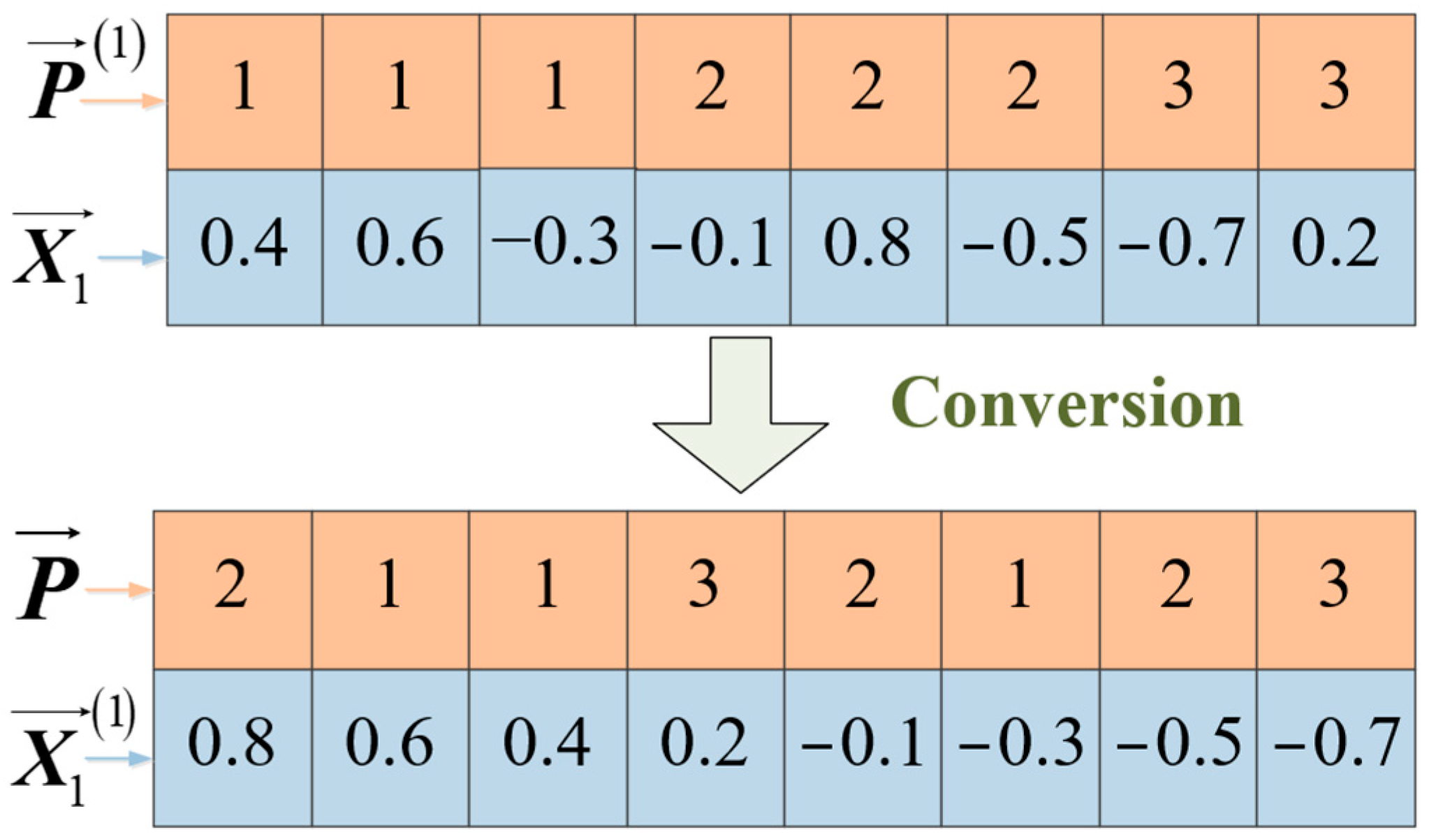
4.2. The Transformation of Chromosome

Due to the nature of the DE algorithm, its chromosomes appear as a real parameter vector ($\overrightarrow{X}=\left[{\overrightarrow{X}}_1,{\overrightarrow{X}}_2,{\overrightarrow{X}}_3,{\overrightarrow{X}}_4\right]=$ [x₁, x₂, …, x_k, …, x_4d] ($x_k\in \left[-\delta ,\delta \right]$)). However, due to the nature of the problem being asked, the chromosomes appear as four integer parameter vectors generated based on the encoding of the processing machine state. Therefore, to facilitate the fitness calculation and the execution of the heuristic strategy, a corresponding conversion method is introduced to realize the mutual conversion between the real parameter vector and the integer parameter vector.

4.2.1. Positive Transformation

The positive transformation is to transform the real-parameter vector to an integer–parameter vector. For the process fragment, this paper proposes a bidirectional sorting rule to transform ${\overrightarrow{X}}_1$ = [x₁, x₂, …, x_d] to $\overrightarrow{P}$ = [p₁, p₂, …, p_d].

First, arrange all process codes in non-decreasing order to generate ${\overrightarrow{P}}^{\left(1\right)}$ and map ${\overrightarrow{X}}_1$ and ${\overrightarrow{P}}^{\left(1\right)}$ to each other. Second, arrange ${\overrightarrow{X}}_1$ in non-incremental order to generate ${{\overrightarrow{X}}_1}^{\left(1\right)}$ and the related mapping ${\overrightarrow{P}}^{\left(1\right)}$ is $\overrightarrow{P}$. An example of process fragment conversion is illustrated in Figure 7.

For the machine fragment, Equation (48) is employed to transform ${\overrightarrow{X}}_2=\left[x\left(d+1\right),x\left(d+2\right),\dots ,xk,\dots ,x2d\right]$ to M = [m₁,m₂, …, m_k, …, m_d]. Where $i_k=m_k$, $\left[-\delta ,\delta \right]$ is the bound of $x_k$ and $l_k$ indicates the quantity of the available machines for the k-th process in $\overrightarrow{P}$. For the machine speed fragment and crane speed fragment, the transformation method is the same as the machine fragment. The parameter $l_k$ denotes the quantity of the machine’s speed level or the quantity of the crane’s speed level in Equation (48) when converting ${\overrightarrow{X}}_3=\left[x2d+1,x2d+2,\dots ,xk,\dots .x3d\right]$ to $\overrightarrow{Q}=\left[q1,q2,\dots ,qk,\dots ,qd\right]$ = or converting ${\overrightarrow{X}}_4=\left[x3d+1,x3d+2,\dots ,xk,\dots ,x4d\right]$ to $\overrightarrow{N}=\left[n1,n2,\dots ,nk,\dots ,nd\right]$.

$$i_k=round\left(\frac{\left(l_k-1\right)\cdot \left(x_k+\delta \right)}{2\delta }+1\right).$$

(48)

4.2.2. Negative Transformation

The negative transformation is to transform the integer–parameter vector to the real-parameter vector. For the process fragment, the transformation from $\overrightarrow{P}$ to ${\overrightarrow{X}}_1$ can be achieved by mapping ${\overrightarrow{P}}^{\left(1\right)}$ ↔${\overrightarrow{X}}_1$. For the fragment of the machine, machine speed, and crane speed, the negative transformation is an inverse linear transformation of the Equation (49). However, it is necessary to regenerate $x_k$ randomly when $l_k=1$.

$$x_k=\left\{\begin{array}{l}\frac{2\delta \left(i_k-1\right)}{l_k-1}-\delta , l_k\ne 1\\ rand(-\delta ,\delta ) , l_k=1\end{array}\right..$$

(49)

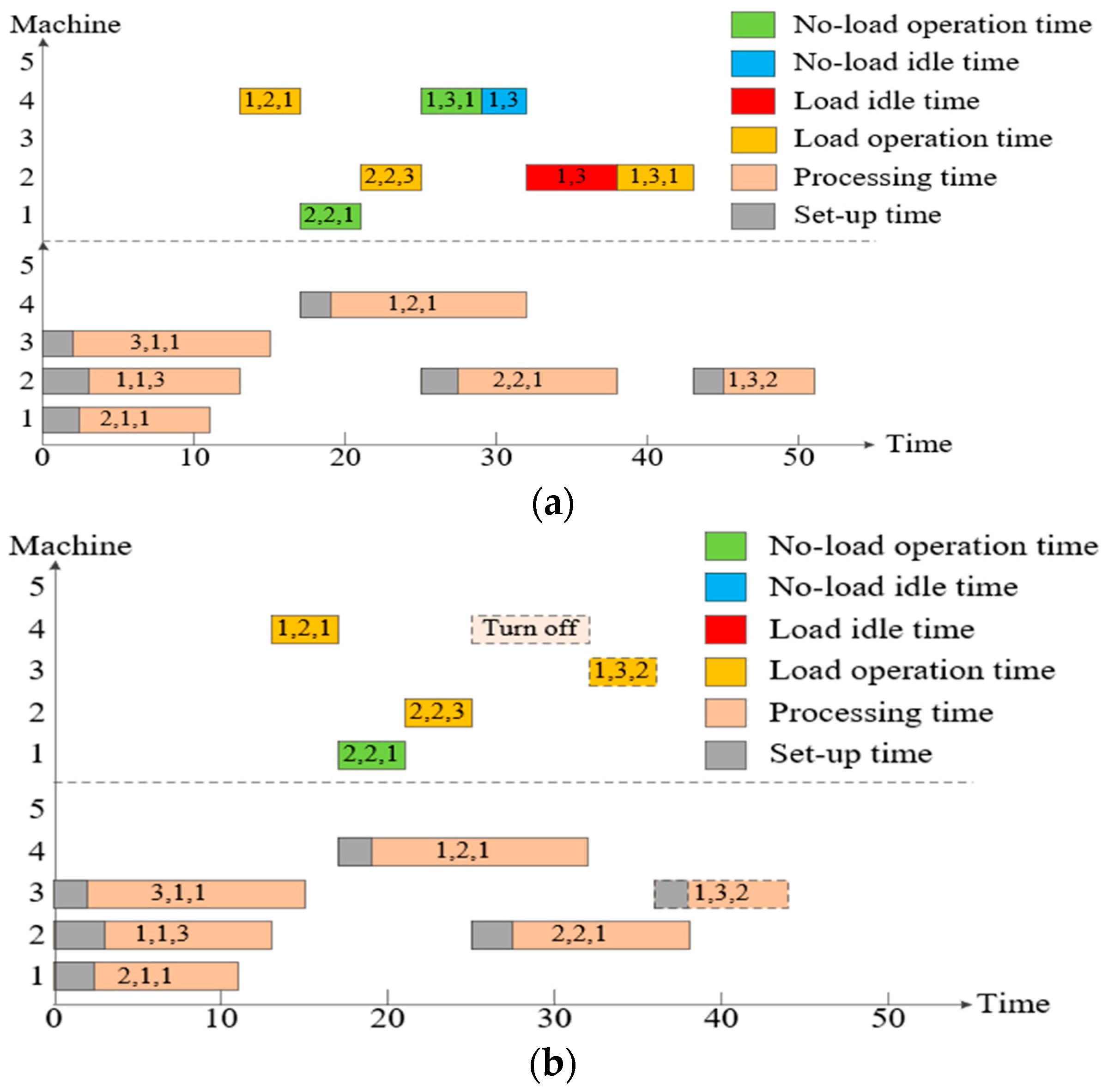
4.3. The Collaborative State Optimization Strategy

The collaborative state optimization strategy is introduced here to guide the search direction for collaboratively optimizing the state of the machine and crane. The CSOS contains two following strategies: load transportation state optimization strategy and machine state optimization strategy. For each process, the two strategies are executed in sequential order to update the chromosome.

4.3.1. Strategy 1: Load Transportation State Optimization Strategy

There is a lot of room for optimization of load energy consumption. This strategy optimizes the energy consumption of the crane load by coordinating the crane operation state. The main principles are: (1) Placing the workpiece to the nearest idle machine can effectively reduce the distance and time of load transport and load idle time; (2) Recon the crane speed for the updated process to optimize the crane operation energy consumption; (3) The crane idle energy consumption is optimized by turning off. The main steps are as follows:

Step 1: Suppose that machine m ($m\in \theta \left(P_{i,n}\right)$) is for P_i,n and the corresponding crane speed level is r in a chromosome, judge whether P_i,n has neighboring available machines (The machine whose load transport distance is not greater than machine m in $\theta \left(P_{i,n}\right)$). If yes, build the neighboring machine set ${\theta }^{\prime }\left(P_{i,n}\right)$ and go to step 2; otherwise, go to step 6.

Step 2: Judge whether there are idle machines in ${\theta }^{\prime }\left(P_{i,n}\right)$ at the completion time of $P_{i-1,n}$ ($T{c}_{i-1,n}$). If yes, go to step 3; otherwise, go to step 6.

Step 3: Construct the process-level comprehensive energy consumption evaluation for the idle machine m′ in ${\theta }^{\prime }\left(P_{i,n}\right)$, as shown in Equations (50) and (51). When the evaluation value is positive, the larger the evaluation value, the lower the comprehensive energy consumption of machine m′ for P_i,n. If there exists at least one idle machine with a positive evaluation value in ${\theta }^{\prime }\left(P_{i,n}\right)$, go to step 4; otherwise, go to step 5.

$$E\left(P_{i,n},m\right)=E^{ms}\left(P_{i,n}\right)+E^{mo}\left(P_{i,n}\right)+E^{mi}\left(P_{i,n}\right)+E^{ci}\left(P_{i,n}\right)+E^{no}\left(P_{i,n}\right)+E^{lo}\left(P_{i,n}\right) , M_{i,n}=m,$$

(50)

$$E\left(P_{i,n},m,m^{\prime }\right)=E\left(P_{i,n},m\right)-E\left(P_{i,n},m^{\prime }\right).$$

(51)

Step 4: Select the idle machine m′ with the highest evaluation value from ${\theta }^{\prime }\left(P_{i,n}\right)$ and replace machine m with machine m′ for P_i,n, go to step 5.

Step 5: Reassign the crane speed level to P_i,n with machine m′. Comprehensively evaluate the load operation energy consumption and time of the crane speed level by Equation (52), and select the speed level r′ with the highest evaluation value to replace the original crane speed level r of P_i,n, go to step 6.

$$F\left(P_{i,n},m^{\prime },r^{\prime }\right)=\frac{1}{E^{lo}\left(P_{i,n}\right)\cdot PE+\left(T_{i,n}^{lo,g}+T_{i,n}^{lo,t}\right)\cdot PT}.$$

(52)

Step 6: Judge whether the crane is in an idle state before load transport ($E^{ci}\left(P_{i,n}\right)\ne 0$). If yes, go to step 7; otherwise, go to step 8.

Step 7: Evaluate $E^{ci}\left(P_{i,n}\right)$ by Equation (53). If the evaluation value is positive, maintain the current idle state of the crane; otherwise, temporarily turn off the crane until load transport begins. Go to step 8.

$$E\left(E^{ci}\left(P_{i,n}\right)\right)=E^{ci}\left(P_{i,n}\right)-E_c^{of}.$$

(53)

Step 8: Perform steps 1–7 for each process in the process order of the chromosome.

To present strategy 1 more intuitively, an instance is introduced in Figure 8.

For the Gantt chart, the upper half of the dotted line indicates the operating path of the crane, and the lower half of the dotted line denotes the processing order of the workpiece. The first two digits of the number denote the operation of the workpiece, and the last digit indicates the speed level. The update effect of strategy 1 is shown in Figure 8b. First, process P_3,1 is rescheduled from machine 2 to machine 3; second, the crane speed level of P_3,1 is reassigned; third, the shutdown status of the crane is determined. Obviously, the updated processing plan not only reduces transport energy consumption but also economizes makespan.

4.3.2. Strategy 2: Machining State Optimization Strategy

Since the machines are reassigned to the process in strategy 1, it is necessary to reallocate the machining state to further the optimization of the machining energy consumption. The detailed steps of the strategy are as follows:

Step 1: Suppose that machine m ($m\in \theta \left(P_{i,n}\right)$) with speed level q is for P_i,n in a chromosome, judge whether machine m needs to be set up for P_i,n. If yes, go to step 2; otherwise, it needs to consider the impact of the resetting time on makespan, go to step 3.

Step 2: Perform process-level machine energy consumption evaluation (54) for machine m with different speed levels. Select the machine speed level q′ with the lowest energy consumption to replace the original speed level q of machine m and go to step 4.

Step 3: Construct the comprehensive evaluation of energy consumption and makespan (55) for machine m with different speed levels. Select the machine speed level q with the lowest evaluation value to replace the original speed level q of machine m and go to step 4.

Step 4: Judge whether machine m is in idle state before P_i,n ($T_{i,n,m}^i\ne 0$). If yes, go to step 5; otherwise, go to step 8.

Step 5: Judge whether machine m needs to be set up for P_i,n. If yes, go to step 6; otherwise, go to step 7.

Step 6: Evaluate the energy consumption of machine state change (idle or power on/off) by Equation (56). Where $E^{ms,of}\left(P_{i,n}\right)$ denotes the restarting set-up energy consumption of machine m. If the energy difference is positive, temporarily turn off machine m until load transport begins; otherwise, maintain the current idle state of machine m. Go to step 8.

Step 7: Comprehensively evaluate the energy consumption and makespan of machine state change by Equation (57). Where $T_{i,n,m,q}^{s,of}$ denotes the restarting set-up time of machine m. If the evaluation value is positive, maintain the current idle state of machine m; otherwise, temporarily turn off machine m until transport begins. Go to step 8.

Step 8: Perform steps 1–3 for each process in the process order of the chromosome.

$$E\left(P_{i,n},m,q\right)=E^{ms}\left(P_{i,n}\right)+E^{mo}\left(P_{i,n}\right)+E^{mi}\left(P_{i,n}\right) , M_{i,n}=m\cap Q_{i,n,m}=q,$$

(54)

$$F\left(P_{i,n},m,q\right)=\left(E^{ms}\left(P_{i,n}\right)+E^{mo}\left(P_{i,n}\right)+E^{mi}\left(P_{i,n}\right)\right)\cdot PE+\left(T_{i,n,m,q}^s+T_{i,n,m,q}^o+T_{i,n,m}^i\right)\cdot PT , M_{i,n}=m\cap Q_{i,n,m}=q,$$

(55)

$$E^{msc}\left(P_{i,n}\right)=E^{mi}\left(P_{i,n}\right)+E^{ms}\left(P_{i,n}\right)-E_m^{of}-E^{ms,of}\left(P_{i,n}\right),$$

(56)

$$F^{msc}\left(P_{i,n}\right)=\left(E_m^{of}+E^{ms,of}\left(P_{i,n}\right)-E^{mi}\left(P_{i,n}\right)-E^{ms}\left(P_{i,n}\right)\right)\cdot PE+\left(T_{i,n,m,q}^{s,of}\right)\cdot PT.$$

(57)

4.4. The Differential Evolution Algorithm

The differential evolution algorithm is a global search algorithm based on group optimization. Similar to GA, differential evolution also has mutation, crossover, and selection operations. However, since all individuals in DE perform genetic mutation operations on each other, DE has stronger optimization and convergence ability than traditional GA, DE has faster convergence speed and more accurate results, and the algorithm is relatively more stable.

4.4.1. Initialization

In the DE algorithm, each individual of a population is represented in the form of a real parameter vector. Since the encoding method proposed in Section 4.2 contains the information on 4d dimensions (d indicates the quantity of all processes), the initialization of the DE algorithm needs to generate real parameter vector individuals on the same dimension. Suppose that $g=0,1,2,\dots ,G$ denotes the generation, $i=1,2,\dots ,4d$ indicates the dimension index of the chromosome and NP is the size of the population. The j-th ($j\in \left\{1,2,\dots ,NP\right\}$) individual in the g-th generation is represented as ${\overrightarrow{X}}_{j,g}=\left[x_{1,j,g},x_{2,j,g},\dots ,x_{i,j,g},\dots ,x_{4d,j,g}\right]$.

The initial population is generated randomly by Equation (58), where $x_{i,max}$ and $x_{i,min}$ denote the upper and lower bound of $x_{i,j,g},$ respectively. Since the corresponding chromosome transformation method has been proposed in Section 4.3, $\left[x_{i,min},x_{i,max}\right]$ is set to $\left[-\delta ,\delta \right]$ to facilitate the operation. Where $\delta$ is served as the bound factor and is set to 1 in this paper.

$$x_{i,j,0}=x_{i,\min }+\left(x_{i,\max }-x_{i,\min }\right)\cdot rand\left(0,1\right).$$

(58)

4.4.2. Mutation

The principle of mutation is to perturb the target vector (a parent vector from the current generation) to generate a mutation vector (${\overrightarrow{V}}_{j,g}=\left[v_{1,j,g},v_{2,j,g},\dots ,v_{4d,j,g}\right]$). Instead of small alterations of chromosomes in GA mutation, the DE mutation is operated using individual composition. This paper chooses the DE/best/2/exp operator for mutation operation (Differential evolution with individual-dependent and dynamic parameter adjustment), which is illustrated in Equation (59), where ${\overrightarrow{X}}_{b,g}$ denotes the best individual (with the beat fitness value) at generation g, $r_1^j,r_2^j,r_3^j,r_4^j\in \left\{1,2,\dots ,NP\right\}$ are the randomly selected individual serial numbers, F is the scaling factor with a value range of [0, 2], which is used to control the disturbance of the difference vector.

$${\overrightarrow{V}}_{j,g}={\overrightarrow{X}}_{b,g}+F\cdot \left({\overrightarrow{X}}_{r_1^j,g}+{\overrightarrow{X}}_{r_2^j,g}-{\overrightarrow{X}}_{r_3^j,g}-{\overrightarrow{X}}_{r_4^j,g}\right).$$

(59)

4.4.3. Crossover

The crossover operation enhances population diversity by randomly recombining the dimensional components of the mutation vector ${\overrightarrow{V}}_{j,g}$ and target vector ${\overrightarrow{X}}_{j,g}$. In this paper, the exponential distribution crossover (exp) is employed to generate a trial vector (${\overrightarrow{U}}_{j,g}=\left[u_{1,j,g},u_{2,j,g},\dots ,u_{4d,j,g}\right]$). The generation method is formulated in Equation (60), where $i_{rand}$ is a random integer in the range [1, 4d] to ensure that the trial vector has at least one-dimensional component different from the target vector, CP denotes the crossover probability, its value is a real number in the range [0, 1].

$$u_{i,j,g}=\left\{\begin{array}{l}{v}_{i,j,g}, \mathrm{from} i=i_{rand} \mathrm{while} rand\left(0, 1\right)\le CP\\ x_{i,j,g}, \mathrm{otherwise}\end{array}\right..$$

(60)

4.4.4. Selection

The selection operation chooses a more adaptive dimensional component from the target vector and the trial vector to enter the offspring through the greedy rule, which is outlined in Equation (61), where $f\left(\overrightarrow{X}\right)$ is the objective function.

$${\overrightarrow{X}}_{j,g+1}=\left\{\begin{array}{l}{\overrightarrow{U}}_{j,g}, \mathrm{if} f\left({\overrightarrow{U}}_{j,g}\right)\le f\left({\overrightarrow{X}}_{j,g}\right)\\ {\overrightarrow{X}}_{j,g}, \mathrm{otherwise}\end{array}\right..$$

(61)

4.5. The Firefly Algorithm

The firefly algorithm was proposed by Xin-She Yang, a Cambridge scholar, and optimized by simulating the group behavior of fireflies. Since the algorithm has a strong local search ability, this algorithm is used in this paper to optimize the offspring generated by DE to mine potential better solutions [45]. In order to improve the problem of slow convergence at the late stage of DE, a detailed collaborative process between algorithms has been developed as shown below.

4.5.1. Algorithm Rules

The firefly algorithm simulates the firefly individuals in nature with the points in the search space and searches the solution space by simulating the attraction and movement process of the firefly individuals. The execution of the algorithm is based on the following principles:

(1) Fireflies have no gender; they are attracted to each other.

(2) The attraction is proportional to their brightness, with each firefly moving towards the brighter individual.

(3) The brightness of fireflies is determined by the objective function.

4.5.2. Parameter Properties

The algorithm simulates the group behavior of fireflies through the following three parameter attributes:

(1) Relative fluorescence intensity:

$$I\left(r_{ij}\right)=I_0\times e^{-\gamma r_{ij}^2},$$

(62)

where $\gamma$ denotes the light absorption coefficient, $I_0$ is the initial fluorescence intensity (at $r_{ij}=0$) negatively related to the objective function value, and $r_{ij}=\Vert x_i-x_j\Vert$ indicates the Cartesian distance between fireflies i and j.

(2) Attractiveness:

$$\beta \left(r_{ij}\right)={\beta }_0\times e^{-\gamma r_{ij}^2},$$

(63)

where ${\beta }_0$ indicates the initial attractiveness constant (at $r_{ij}$= 0), it is set to 1 in this paper.

(3) Location update:

$$x_i=x_i+\beta \left(r_{ij}\right)\times \left(x_j-x_i\right)+\alpha \times \left(rand-0.5\right),$$

(64)

where $\alpha$ denotes the random step factor, $rand$ is a random number that satisfies uniform distribution in [0, 1].

4.6. Complexity Analysis

The time requirement of the algorithm is called the time complexity of the algorithm. It is an important index to evaluate the feasibility of the algorithm. Here, we analyze the computational complexity of each block and then aggregate the modules to obtain the total complexity of the DE-FA-CSOS algorithm. In one generation, the complexity of DE-FA-CSOS is influenced by the following factors: the number of populations, the number of generations, the number of machines, the number of jobs, and the maximal operation number. Hence, the computational complexity of DE-FA-CSOS at worst is O (2RSMN²max{P_n}²). Where R is the population size, S is the total number of iterations, M is the number of machines, N is the number of workpieces, and Pn is the number of processes of workpiece n.

5. Case Study

In this section, the performance and optimization effects of the proposed low-carbon scheduling method are demonstrated by a detailed case study and corresponding comparative experiments. All experiments are coded in MATLAB R2018b and run on a 2.2 GHz CPU with 16G RAM in the Windows 10 platform.

5.1. Data Source

Since the problem studied in this paper has an industrial application background, the data sources are obtained in a large cement equipment manufacturing company [4]. The company mainly produces large-scale cement production equipment and its components, e.g., roller presses, rotary kilns, vertical mills, etc. Through investigation, the machining mode of the workshop is a flexible environment (the machines have multiple functions and multiple adjustable states), and the means of transportation in the workshop is an overhead crane with multiple states. The case study investigates the processes of 50 sets of common production tasks in the company to conduct experiments.

The detailed parameters of the machines in the workshop are listed in Table 1. Due to the discrete processing time of the machining process, that is, the machines do not run continuously at rated power during the statistical processing time, the operating power of the machine listed in Table 1 is the average power of the machine running at a certain speed. The detailed parameters of the crane inside the workshop are as follows:

(1) Crane’s gantry parameters: speed level 1, running speed 25 m/min, running power 4700 W; speed level 2, running speed 50 m/min, and running power 8000 W.

(2) Crane’s trolley parameters: speed level 1, running speed 15 m/min, running power 2800 W; speed level 2, running speed 30 m/min, and running power 5000 W.

(3) Crane’s general parameters: idle power 750 W, startup energy consumption 150 kJ, lifting appliance mass 900 kg, rated lifting mass 10,000 kg, gantry mass 9746 kg, and trolley mass 5493 kg.

Table 1. The parameters of machines in the case workshop.

Machine	Level 1 Power (W)		Level 2 Power (W)		Level 3 Power (W)		Location (m)		Set Up		Startup Energy (kJ)
	Operating	Idle	Operating	Idle	Operating	Idle	Dxm	Dym	Time (min)	Power (W)
1	1120	220	1690	280	1960	390	30	20	1	240	141.6
2	1340	240	1870	310	2320	340	30	80	2	190	133.8
3	1050	180	1520	290	1920	350	130	20	1	210	124.8
4	1210	210	1780	330	2070	410	130	80	1	230	165.6
5	1170	230	1590	270	2260	320	230	20	1	210	118.2
6	1290	190	1810	320	2470	310	230	80	2	180	150.6

Table 1. The parameters of machines in the case workshop.

Machine	Level 1 Power (W)		Level 2 Power (W)		Level 3 Power (W)		Location (m)		Set Up		Startup Energy (kJ)
	Operating	Idle	Operating	Idle	Operating	Idle	Dxm	Dym	Time (min)	Power (W)
1	1120	220	1690	280	1960	390	30	20	1	240	141.6
2	1340	240	1870	310	2320	340	30	80	2	190	133.8
3	1050	180	1520	290	1920	350	130	20	1	210	124.8
4	1210	210	1780	330	2070	410	130	80	1	230	165.6
5	1170	230	1590	270	2260	320	230	20	1	210	118.2
6	1290	190	1810	320	2470	310	230	80	2	180	150.6

5.2. Performance Comparison Analysis

To demonstrate the performance of DE-FA-CSOS, the comparison experiment analyzes the solution quality, efficiency, and stability of it. Since it is difficult to find other algorithms to solve this problem, the random state matching strategy is embedded in the state-of-the-art workshop scheduling algorithms for comparative analysis.

(1) DE-FA-CSOS.

(2) DE-FA: the hybrid DE-FA algorithm with a random state matching strategy.

(3) ABC: the artificial bee colony algorithm with random state matching strategy.

(4) DE: the differential evolution algorithm with random state matching strategy.

(5) PSO: the particle swarm optimization algorithm with random state matching strategy.

5.2.1. Parameter Setting

Since the algorithm parameters have a significant influence on the algorithm performance, the Taguchi method is used to conduct parameter adjustment experiments for the comparison algorithms [46]. The parameter combinations optimized by the Taguchi method are as follows: The population size of all the compared algorithms is set to 100. The number of iterations is set to 5000. In DE-FA-CSOS and DE-FA, the parameters of the DE are as follows: the crossover probability and scaling factor are set as 0.8 and 0.5, respectively. The algorithm parameters of the FA are set as follows: the light absorption coefficient is set as 0.06, the initial attractiveness constant is set as 1, and the random step factor is set to 1.2. In ABC, the control parameter $limit=25$, and the colony size of onlooker bees is 50. In DE, the scaling factor F = 0.5 and the crossover probability CP = 0.5. In PSO, the inertia weight w = 0.6, learning factors c1 = c2 = 2, and maximal velocity V_max = 0.1.

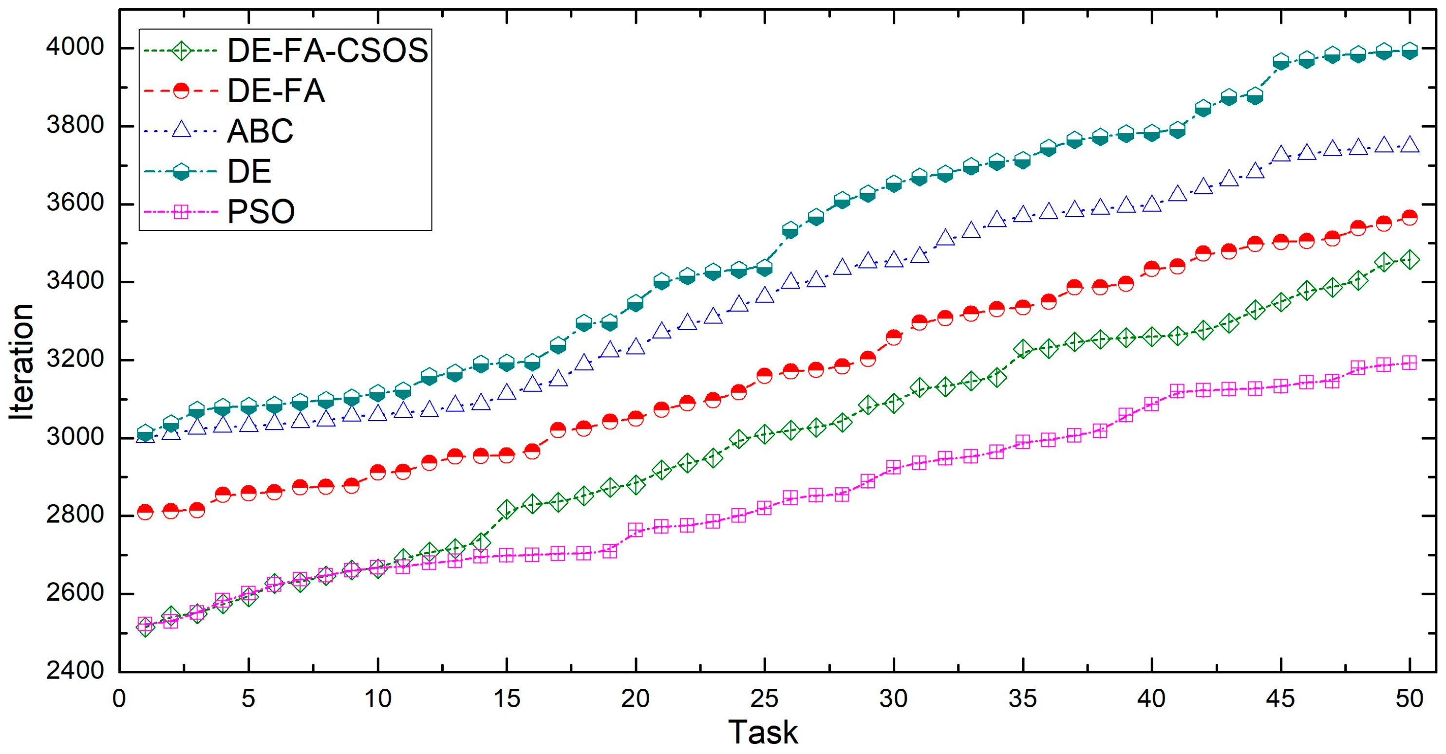
5.2.2. Comparison Results Analysis

To avoid the randomness influence on the result analysis of the compared algorithms, the 50 groups of experiments were run 20 times independently.

Table 2. The optimization results of the compared algorithms.

Task	DE-FA-CSOS		DE-FA		ABC		DE		PSO
	Mean	Std	Mean	Std	Mean	Std	Mean	Std	Mean	Std
1	40.06	0.902	40.10	1.091	41.01	1.079	40.37	1.343	40.25	1.110
2	40.39	0.992	40.55	1.174	41.16	1.098	40.40	1.178	40.39	1.341
3	40.60	0.883	41.35	1.118	41.27	1.378	41.60	1.352	42.20	1.176
4	41.30	0.954	41.87	1.014	41.36	1.293	41.76	1.317	42.70	1.175
5	41.81	0.911	41.67	1.007	41.51	1.196	42.32	1.248	43.12	1.253
6	41.93	0.849	41.73	1.048	41.93	1.379	42.77	1.277	43.77	1.277
7	42.01	1.064	42.27	1.089	42.31	1.356	42.96	1.181	44.61	1.181
8	42.51	0.808	43.37	1.020	42.61	1.307	43.73	1.138	44.71	1.200
9	42.62	1.037	43.61	1.147	42.92	1.110	44.45	1.237	45.16	1.437
10	43.04	0.878	43.64	1.145	44.42	1.379	44.74	1.347	45.30	1.122
11	43.52	1.059	44.51	1.001	44.54	1.075	44.77	1.242	45.77	1.481
12	43.77	0.912	44.90	1.061	45.81	1.237	45.31	1.156	45.92	1.307
13	43.97	0.939	45.33	1.163	46.13	1.193	46.03	1.139	45.98	1.210
14	44.19	1.063	45.60	1.118	46.16	1.227	46.91	1.397	46.42	1.304
15	44.45	0.905	45.93	1.025	46.66	1.072	47.02	1.124	47.08	1.338
16	44.57	0.902	46.02	1.147	47.47	1.236	47.24	1.390	47.50	1.149
17	45.37	0.806	46.31	1.102	47.91	1.267	47.28	1.206	48.40	1.391
18	45.44	0.963	46.80	1.124	48.50	1.354	47.33	1.234	48.47	1.386
19	45.95	0.801	46.90	1.053	48.63	1.066	47.61	1.278	48.93	1.277
20	46.13	0.903	46.92	1.049	48.83	1.201	48.00	1.161	48.95	1.462
21	46.80	1.054	47.09	1.119	49.09	1.078	48.40	1.288	49.04	1.214
22	47.20	1.056	47.12	1.085	49.39	1.287	48.69	1.374	49.83	1.102
23	47.29	1.029	47.37	1.067	49.43	1.368	48.81	1.299	49.84	1.104
24	47.53	1.019	47.93	1.059	49.76	1.118	49.32	1.114	51.16	1.294
25	48.08	0.976	48.34	1.066	49.78	1.012	49.95	1.307	51.49	1.258
26	48.53	0.954	48.55	1.116	49.90	1.170	50.00	1.207	52.54	1.186
27	48.91	0.925	48.99	1.158	50.28	1.142	50.02	1.176	52.65	1.443
28	49.20	0.935	50.56	1.149	50.40	1.232	50.67	1.288	53.02	1.423
29	50.78	1.027	51.20	1.029	50.83	1.239	51.60	1.291	53.14	1.330
30	50.95	1.054	51.80	1.022	51.33	1.220	51.69	1.108	53.33	1.240
31	51.17	0.816	51.89	1.108	51.45	1.373	51.95	1.155	54.36	1.494
32	51.46	0.844	52.63	1.073	52.75	1.020	52.26	1.246	54.91	1.405
33	51.82	0.803	53.22	1.151	52.84	1.106	52.52	1.326	54.98	1.347
34	51.93	0.823	53.81	1.131	53.05	1.355	52.53	1.163	55.18	1.103
35	52.74	0.994	53.94	1.028	53.43	1.264	53.48	1.285	55.48	1.226
36	53.49	0.845	54.48	1.115	53.57	1.097	53.58	1.243	55.50	1.238
37	53.80	1.075	54.67	1.065	54.24	1.023	53.80	1.150	55.59	1.402
38	53.97	1.003	54.70	1.006	56.77	1.144	54.28	1.242	55.68	1.242
39	54.49	0.806	54.99	1.145	56.92	1.174	54.96	1.163	55.94	1.423
40	55.43	0.990	55.26	1.143	56.95	1.092	55.84	1.369	56.31	1.465
41	55.67	1.031	55.82	1.120	57.21	1.012	55.93	1.384	57.51	1.245
42	55.84	0.910	55.98	1.191	57.34	1.120	56.17	1.245	57.61	1.312
43	56.16	1.059	56.54	1.001	57.36	1.043	56.37	1.175	57.64	1.284
44	56.76	0.837	56.87	1.173	57.72	1.327	57.69	1.252	57.75	1.294
45	56.81	0.998	56.95	1.159	57.95	1.009	57.74	1.271	58.04	1.273
46	57.53	1.090	57.93	1.160	58.07	1.150	57.95	1.102	58.54	1.402
47	57.77	0.930	58.20	1.132	58.84	1.232	58.09	1.108	58.84	1.312
48	58.31	0.910	59.03	1.087	59.25	1.184	58.89	1.178	58.91	1.139
49	58.97	1.025	59.18	1.062	59.41	1.346	59.55	1.284	59.44	1.292
50	59.21	0.843	59.72	1.048	59.64	1.214	59.77	1.328	59.48	1.158
Best/All	46/50	45/50	3/50	3/50	1/50	2/50	0/50	0/50	0/50	0/50
Friedman	1.13	1.14	2.56	2.32	3.46	3.36	3.25	3.91	4.60	4.27

lists the optimization results of the comparison algorithms. Figure 9 shows the average convergence iterations of the compared algorithms.

As shown in the table and figure, PSO has the fastest convergence rate in 50 production task examples. However, its optimization quality is inferior to that of other comparison algorithms, with a total rank in the mean value of 4.60 when it comes to the Friedman test. This proves that the convergence speed of PSO is fast, but it is prone to fall into pre-mature convergence. The solution quality of ABC and DE is better than PSO, with total ranks in the mean value of 3.46 for ABC and 3.25 for DE, but their convergence efficiencies are relatively low. The DE-FA algorithm integrates the global search of DE and the local search of FA so that its convergence speed is relatively ideal and its optimization results are better than ABC, DE, and PSO with a total rank in the mean value of 2.56. Due to the increased CSOS guiding the search direction of the DE-FA, the DE-FA-CSOS has better search performance and convergence ability than the DE-FA, leading to 1.43 on total rank in the mean value and 200 on convergence iteration.

Moreover, it is shown in Table 2 that the DE-FA-CSOS has the best total ranks in both mean value and std value, which verifies that the DE-FA-CSOS has advantages in both performance and stability compared with other algorithms. Consequently, the conclusions are summarized as follows:

(1) The DE-FA has a better search ability than the ABC, DE, and PSO in the LSP-FM&CT-MCC, which provides a basic guarantee for the embedding of CSOS.

(2) The addition of CSOS further improves the performance and stability of the DE-FA algorithm in the LSP-FM&CT-MCC.

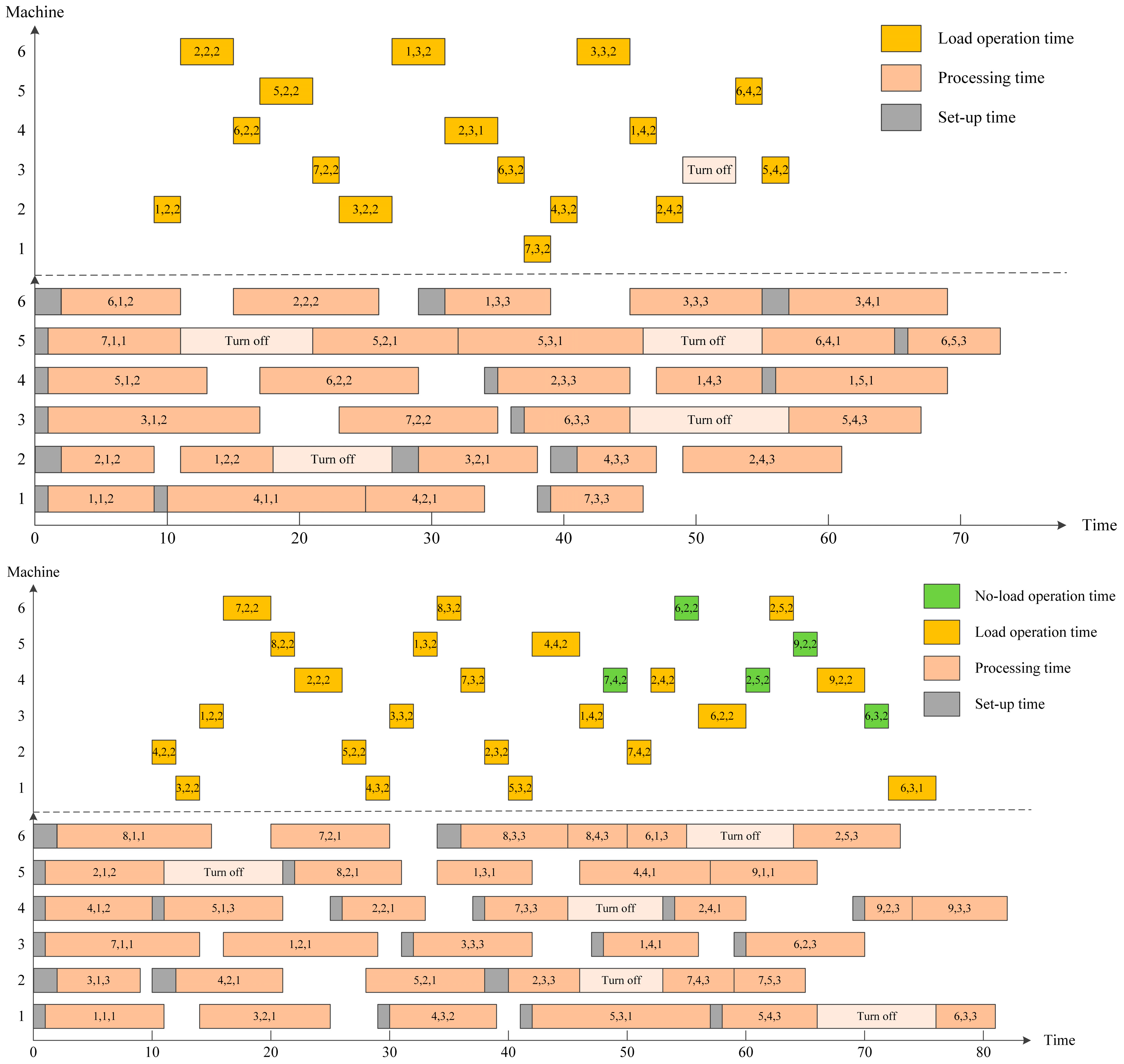
5.3. Scheduling Solution Analysis

In the above comparison experiment, the DE-FA-CSOS has better solution quality than DE-FA due to the addition of CSOS. In this section, the specific scheduling effects of DE-FA-CSOS are analyzed through the Gantt Chart of optimization solutions to demonstrate the practical role of CSOS. Figure 10 shows the Gantt chart of optimal scheduling solutions of DE-FA-CSOS for two typical production tasks with the highest frequency of execution.

As shown in Figure 10, with the application of the load transportation state optimization strategy in CSOS, the crane’s transportation process has been optimized well. First, the workpiece is inserted into the nearby idle machine, effectively reducing the load transportation distance of the crane, and avoiding the load idle time. Then, the crane’s running speed for the updated process is reconfigured to make the crane operation more continuous. Meanwhile, since the machine is reassigned for the process in the load transportation state optimization strategy, the implementation of the machining state optimization strategy in CSOS synchronously configures the states of updated machines. Under the cooperation of the two strategies, the multiple operating states of the crane and machines achieve an optimal balance. The GIA interactive rate of various equipment in the workshop is improved, and the makespan is significantly reduced. Therefore, the application of the two strategies in CSOS has a good collaborative optimization effect and plays an obvious role in scheduling optimization.

5.4. Low-Carbon Optimization Effect Analysis

To further verify the effect of DE-FA-CSOS on low-carbon optimization, the two strategies in CSOS are added to the DE-FA, respectively, to conduct a compared experiment. The four combinational algorithms are compared in terms of different types of energy consumption, which can be defined as follows.

(1) DE-FA-CSOS.

(2) DE-FA-S1: the hybrid DE-FA algorithm with strategy 1: load transportation state optimization strategy.

(3) DE-FA-S2: the hybrid DE-FA algorithm with strategy 2: machining state optimization strategy.

(4) DE-FA: the hybrid DE-FA algorithm with a random state matching strategy.

Figure 11 shows the results of different types of energy consumption during the machining process optimized by the above four algorithms. Obviously, in Figure 11, these four algorithms have their own characteristics for the optimization of energy consumption. For the machining energy consumption shown in Figure 11a, the effect ranking of the four algorithms is DE-FA-CSOS > DE-FA-S2 = DE-FA-S1 > DE-FA. Since both the DE-FA-CSOS and the DE-FA-S2 contain the machining state optimization strategy, their machining energy efficiencies are better than the DE-FA-S1 and the DE-FA. Specifically, the application of the machining state optimization strategy has significantly reduced the machine energy consumption of operation, setup, and turn-on/off.

As shown in Figure 11b, due to the DE-FA-CSOS and DE-FA-S1 containing the load transportation state optimization strategy, their transportation energy efficiencies are better than the DE-FA-S2 and the DE-FA. For the energy consumption of load and no-load operation, the optimization results from the DE-FA-CSOS and DE-FA-S1 are significantly lower than the DE-FA-S2 and DE-FA. For the energy consumption of the crane idle and turn on/off, the optimization results from the DE-FA-CSOS are 0, which have distinct advantages over the DE-FA-S1, DE-FA-S2, and DE-FA. In terms of the total crane transportation energy consumption, the optimization capability ranking of these four algorithms is DE-FA-CSOS > DE-FA-S1 > DE-FA-S2 > DE-FA. Therefore, the conclusions are summarized as follows:

(1) The strategy 1 and strategy 2 in CSOS have effectively optimized the energy consumption of machining and transportation, respectively, which shows that the two strategies play an important role in the algorithm operation.

(2) The DE-FA-CSOS has better low-carbon optimization capability than the hybrid DE-FA algorithms with separate strategy 1 or strategy 2.

5.5. Algorithm Robustness Analysis

This section examines the robustness of the DE-FA-CSOS for the LSP-FM&CT-MCC in different optimization environments. Since the considerations of energy consumption and makespan are different in diverse manufacturing environments, the dynamic weights of the two objectives are considered to simulate different optimization environments of LSP-FM&CT-MCC. The coefficient $\lambda$ is increased in the objective function as the weight to integrate the two objectives as shown in Equation (65). By changing the value of coefficient $\lambda$ with a step size of 0.05, 19 sets of weights are obtained. The objective function is conducted with the coefficient $\lambda$ from 0.05 to 0.95 so that the optimized solutions are from energy-saving oriented to makespan-saving oriented.

$$\min F=\lambda \times E\times PE+\left(1-\lambda \right)\times M\times PT.$$

(65)

To avoid the influence of the algorithm randomness, the experiments of each set of weights were run 20 times independently and retained the mean values.

Table 3. The statistics of optimization results with different weights.

No.	$\mathit{\lambda }$	DE-FA-CSOS			Solution Gap (%)			DE-FA
		E	M	F	GapE	GapM	GapF	E	M	F
1	0.05	14.62	1.24	26.25	6.91	7.26	7.24	15.63	1.33	28.14
2	0.10	14.34	1.27	26.96	5.72	6.30	6.24	15.16	1.35	28.64
3	0.15	13.83	1.28	27.13	7.52	6.25	6.45	14.87	1.36	28.88
4	0.20	13.28	1.31	27.48	7.00	3.82	4.45	14.21	1.36	28.71
5	0.25	12.72	1.33	27.50	6.76	3.76	4.47	13.58	1.38	28.74
6	0.30	12.39	1.35	27.51	7.18	2.96	4.14	13.28	1.39	28.65
7	0.35	11.85	1.37	27.25	9.79	2.92	5.08	13.01	1.41	28.64
8	0.40	11.59	1.38	26.95	7.77	2.90	4.63	12.49	1.42	28.19
9	0.45	11.14	1.40	26.51	8.62	2.86	5.10	12.10	1.44	27.86
10	0.50	11.08	1.41	26.23	5.51	2.84	4.00	11.69	1.45	27.28
11	0.55	10.83	1.43	25.80	7.39	2.80	4.98	11.63	1.47	27.08
12	0.60	10.52	1.45	25.20	10.08	2.76	6.54	11.58	1.49	26.84
13	0.65	10.34	1.46	24.59	10.93	4.79	8.25	11.47	1.53	26.62
14	0.70	10.31	1.48	24.21	10.77	4.73	8.44	11.42	1.55	26.25
15	0.75	10.30	1.49	23.75	3.50	5.37	4.11	10.66	1.57	24.73
16	0.80	10.04	1.51	22.90	5.08	5.30	5.14	10.55	1.59	24.08
17	0.85	9.86	1.53	22.10	4.16	5.23	4.39	10.27	1.61	23.07
18	0.90	9.75	1.56	21.37	4.00	4.49	4.07	10.14	1.63	22.24
19	0.95	9.69	1.58	20.64	4.02	6.33	4.21	10.08	1.68	21.51
Mean		11.50	1.41	25.28	6.98	4.40	5.36	12.31	1.47	26.64
Std		1.60	0.10	2.21	2.31	1.47	1.41	1.75	0.11	2.37

shows the statistics of the optimization results of the DE-FA-CSOS and the DE-FA for the objective function with different weights, and Figure 12 shows the distribution of solutions with different weights optimized by the DE-FA-CSOS and the DE-FA. As observed in Table 3, the energy consumption from the DE-FA-CSOS is better optimized than DE-FA, the mean gap is 6.98%. The makespan obtained from DE-FA is larger than those obtained from DE-FA-CSOS, the mean gap is 4.40%. Furthermore, as observed in Figure 12, DE-FA-CSOS is distinctly better than DE-FA for both the energy consumption and makespan in every set of weights. The DE-FA-CSOS can maintain the advantages of the optimization effects with the continuous change of the optimization environment. Consequently, the above experiments demonstrate that the DE-FA-CSOS has good robustness and can adapt to the dynamic manufacturing environment.

6. Discussion

In the cement equipment manufacturing company under investigation, the scheduling task of various equipment in the workshop is completed by manual scheduling. This scheduling mode restricts the low-carbon transformation of the manufacturing enterprise. First, the dispatchers’ personal experience is limited. They only arrange the machine for the next process when one workpiece completes the current machining. This kind of local manual decision-making leads to a large waste of machining energy consumption and easily causes a large amount of idle equipment. Second, due to the limited decision-making ability of dispatchers, they are only responsible for the allocation of machines, and ids difficult to comprehensively consider the multiple states of machines and cranes for collaborative configuration, resulting in a waste of transportation energy. Third, the response rate of manual scheduling is much lower than the proposed low-carbon scheduling method, which directly production efficiency and increases the makespan of products. The above similar manual scheduling mode is widely used in traditional manufacturing enterprises, which undoubtedly increases energy waste and excessive carbon emissions.

To prove the effectiveness of the DE-FA-CSOS algorithm proposed in this paper, we improve others’ algorithms and use them for experimental comparison. In Section 5.2 Performance comparison analysis, the comparison experiment analyzes the solution quality, efficiency, and stability of the DE-FA-CSOS, DE-FA, DE [47], ABC [48], and PSO [49] algorithms. The experimental results show that: “(1) The DE-FA has a better search ability than the ABC, DE, and PSO in the LSP-FM&CT-MCC, which provides a basic guarantee for the embedding of CSOS. (2) The addition of CSOS further improves the performance and stability of the DE-FA algorithm in the LSP-FM&CT-MCC.” In Section 5.4, Low-carbon optimization effect analysis, to further verify the effect of DE-FA-CSOS on low-carbon optimization, the two strategies in CSOS are added to the DE-FA, respectively, to conduct a comparison experiment. The four combinational algorithms are compared in terms of different types of energy consumption. The experimental results show that: “(1) The Strategy 1 and Strategy 2 in CSOS have effectively optimized the energy consumption of machining and transportation, respectively, which shows that the two strategies play an important role in the algorithm operation. (2) The DE-FA-CSOS has better low-carbon optimization capability than the hybrid DE-FA algorithms with separate strategy 1 or strategy 2”. In Section 5.4, Low-carbon optimization effect analysis, the experiments demonstrate that the DE-FA-CSOS has good robustness and can adapt to the dynamic manufacturing environment.

Table 4. The comparison of the DE-FA-CSOS and the dispatcher mode.

Task	DE-FA-CSOS			Result Gap (%)			Dispatcher Mode
	Em	Ec	M	GapEm	GapEc	GapM	Em	Ec	M
1	8.69	1.89	1.37	34.46	28.41	29.38	13.26	2.64	1.94
2	11.38	3.52	1.52	25.03	27.12	29.95	15.18	4.83	2.17
3	9.18	3.46	1.45	34.29	36.86	38.30	13.97	5.48	2.35
4	11.08	2.03	1.48	23.95	45.28	40.08	14.57	3.71	2.47
5	13.03	2.85	1.38	19.91	39.87	43.44	16.27	4.74	2.44
6	12.64	3.77	1.47	26.64	21.13	39.26	17.23	4.78	2.42
7	11.61	3.23	1.39	22.13	30.69	39.30	14.91	4.66	2.29
8	12.75	3.56	1.41	18.01	33.46	33.80	15.55	5.35	2.13
9	12.79	2.51	1.42	17.59	45.79	36.61	15.52	4.63	2.24
10	11.66	2.57	1.54	29.63	36.54	40.08	16.57	4.05	2.57
Mean gap				25.17	34.52	37.02
Max gap				34.46	45.79	43.44
Min gap				17.59	21.13	29.38

lists the scheduling results of the DE-FA-CSOS and the dispatcher mode. By comparing the actual application of 10 scheduling tasks, the results show that the machining energy consumption and the transportation energy consumption are reduced by 25.17% and 34.52% on average with the application of the DE-FA-CSOS. This proves that the DE-FA-CSOS effectively improves workshop energy efficiency and reduces carbon emissions. Furthermore, the makespan from DE-FA-CSOS is reduced by 37.02% on average compared with manual methods, which shows that the proposed scheduling method effectively improves the production efficiency of the workshop. Therefore, the DE-FA-CSOS effectively ameliorates the drawbacks of the dispatcher mode and can serve as a reference to promote low-carbon and green development for China’s traditional manufacturing enterprises.

7. Conclusions

To promote the low-carbon transition of the heavy manufacturing industry, this paper introduces a novel LSP-FM&CT-MCC based on a heavy cement equipment manufacturing enterprise. The novelty of this problem is that it considers not only collaborative scheduling optimization of machines and cranes but also the multi-state configuration optimization of multifunctional machines and variable-speed cranes. Due to the more comprehensive consideration, the quality and feasibility of the solution can be greatly improved. In addition, a novel hybrid differential evolution algorithm and firefly algorithm with a collaborative state optimization strategy (DE-FA-CSOS) are proposed in this paper.

The research objective of this paper is to minimize the total energy consumption and makespan of the production process, which in turn reduces carbon emissions for the proposed problem. A new mixed integer planning (MIP) model is established for the proposed problem. In the MIP model, a multi-state integrated energy consumption model based on machining machines and cranes is established to describe the integrated energy consumption of machine and crane operation processes in detail. Since there is no effective solving method, a novel hybrid DE-FA-CSOS algorithm is developed to solve it. An experimental study is conducted with a real production case to verify that the DE-FA-CSOS algorithm can solve the problem in a reasonable time frame and obtain a higher-quality solution. Through repeated comparative experiments, the results show that the machining energy consumption and transportation energy consumption are reduced by 25.17% and 34.52% on average. Compared with manual scheduling, the optimized makespan is shortened by 37.02% on average. This proves that the method in this paper effectively improves the workshop’s energy efficiency and reduces carbon emissions. Therefore, the proposed method has a wide application background in various heavy manufacturing enterprises and is an important guideline for the low-carbon manufacturing of traditional heavy industry.

In terms of the limitations in this paper, the proposed LSP-FM&CT-MCC does not consider the optimization problem of collaborative scheduling of multi-crane transport; it does not take into account the repair and maintenance time of the equipment; the handling of conflicts during machining and transportation has not been fully considered. Additionally, for different machining environments, the effect of order insertion factors should be considered, and the ambiguity of machining time should be reflected in the mathematical model. Concerning the above limitations, the suggestions for further research are as follows:

(1) Study the problem of the multi-state shop and multi-crane transportation collaborative scheduling optimization.

(2) Consider the repair and maintenance time of the equipment in the next step of the study.

(3) Consider handling conflicts in processing and transportation processes in mathematical models.

(4) Considering the effect of order insertion factors in mathematical models.

(5) To apply fuzzy theory to determine the machining time based on the actual machining environment.

(6) Extend this study to other types of shops in the manufacturing industry.

References

1. China Statistical Yearbook; National Bureau of Statistics of China: Beijing, China, 2022.
2. Peng, C.; Guo, X.; Long, H. Carbon Intensity and Green Transition in the Chinese Manufacturing Industry. Energies 2022, 15, 6012. [Google Scholar] [CrossRef]
3. Liu, Y.; Guo, R.; Pan, W. Evaluation of Carbon Emission Efficiency and Spatial Relevance in the Thermal Power Industry: Evidence from China. Environ. Dev. Sustain. 2023. [Google Scholar] [CrossRef]
4. Liu, Z.; Guo, S.; Wang, L. Integrated Green Scheduling Optimization of Flexible Job Shop and Crane Transportation Considering Comprehensive Energy Consumption. J. Clean. Prod. 2019, 211, 765–786. [Google Scholar] [CrossRef]
5. Tirkolaee, E.B.; Goli, A.; Weber, G.-W. Fuzzy Mathematical Programming and Self-Adaptive Artificial Fish Swarm Algorithm for Just-in-Time Energy-Aware Flow Shop Scheduling Problem with Outsourcing Option. IEEE Trans. Fuzzy Syst. 2020, 28, 2772–2783. [Google Scholar] [CrossRef]
6. Yu, T.-S.; Han, J.-H. Scheduling Proportionate Flow Shops with Preventive Machine Maintenance. Int. J. Prod. Econ. 2021, 231, 107874. [Google Scholar] [CrossRef]
7. Fu, Y.; Zhou, M.; Guo, X.; Qi, L. Scheduling Dual-Objective Stochastic Hybrid Flow Shop with Deteriorating Jobs via Bi-Population Evolutionary Algorithm. IEEE Trans. Syst. Man Cybern.-Syst. 2020, 50, 5037–5048. [Google Scholar] [CrossRef]
8. Han, Y.; Li, J.; Sang, H.; Liu, Y.; Gao, K.; Pan, Q. Discrete Evolutionary Multi-Objective Optimization for Energy-Efficient Blocking Flow Shop Scheduling with Setup Time. Appl. Soft. Comput. 2020, 93, 106343. [Google Scholar] [CrossRef]
9. Shao, W.; Shao, Z.; Pi, D. An Ant Colony Optimization Behavior-Based MOEA/D for Distributed Heterogeneous Hybrid Flow Shop Scheduling Problem Under Nonidentical Time-of-Use Electricity Tariffs. IEEE Trans. Autom. Sci. Eng. 2022, 19, 3379–3394. [Google Scholar] [CrossRef]
10. Huang, J.-P.; Pan, Q.-K.; Miao, Z.-H.; Gao, L. Effective Constructive Heuristics and Discrete Bee Colony Optimization for Distributed Flowshop with Setup Times. Eng. Appl. Artif. Intell. 2021, 97, 104016. [Google Scholar] [CrossRef]
11. Li, Y.; Li, X.; Gao, L.; Meng, L. An Improved Artificial Bee Colony Algorithm for Distributed Heterogeneous Hybrid Flowshop Scheduling Problem with Sequence-Dependent Setup Times. Comput. Ind. Eng. 2020, 147, 106638. [Google Scholar] [CrossRef]
12. Wu, X.; Yuan, Q.; Wang, L. Multiobjective Differential Evolution Algorithm for Solving Robotic Cell Scheduling Problem with Batch-Processing Machines. IEEE Trans. Autom. Sci. Eng. 2021, 18, 757–775. [Google Scholar] [CrossRef]
13. Pan, Y.; Gao, K.; Li, Z.; Wu, N. Improved Meta-Heuristics for Solving Distributed Lot-Streaming Permutation Flow Shop Scheduling Problems. IEEE Trans. Autom. Sci. Eng. 2023, 20, 361–371. [Google Scholar] [CrossRef]
14. Qin, M.; Wang, R.; Shi, Z.; Liu, L.; Shi, L. A Genetic Programming-Based Scheduling Approach for Hybrid Flow Shop with a Batch Processor and Waiting Time Constraint. IEEE Trans. Autom. Sci. Eng. 2021, 18, 94–105. [Google Scholar] [CrossRef]
15. Afsar, S.; Jose Palacios, J.; Puente, J.; Vela, C.R.; Gonzalez-Rodriguez, I. Multi-Objective Enhanced Memetic Algorithm for Green Job Shop Scheduling with Uncertain Times. Swarm Evol. Comput. 2022, 68, 101016. [Google Scholar] [CrossRef]
16. Wei, Z.; Liao, W.; Zhang, L. Hybrid Energy-Efficient Scheduling Measures for Flexible Job-Shop Problem with Variable Machining Speeds. Expert Syst. Appl. 2022, 197, 116785. [Google Scholar] [CrossRef]
17. Duan, J.; Wang, J. Energy-Efficient Scheduling for a Flexible Job Shop with Machine Breakdowns Considering Machine Idle Time Arrangement and Machine Speed Level Selection. Comput. Ind. Eng. 2021, 161, 107677. [Google Scholar] [CrossRef]
18. Wu, X.; Peng, J.; Xiao, X.; Wu, S. An Effective Approach for the Dual-Resource Flexible Job Shop Scheduling Problem Considering Loading and Unloading. J. Intell. Manuf. 2021, 32, 707–728. [Google Scholar] [CrossRef]
19. Luo, S.; Zhang, L.; Fan, Y. Real-Time Scheduling for Dynamic Partial-No-Wait Multiobjective Flexible Job Shop by Deep Reinforcement Learning. IEEE Trans. Autom. Sci. Eng. 2022, 19, 3020–3038. [Google Scholar] [CrossRef]
20. Jiang, S.-L.; Liu, Q.; Bogle, I.D.L.; Zheng, Z. A Self-Learning Based Dynamic Multi-Objective Evolutionary Algorithm for Resilient Scheduling Problems in Steelmaking Plants. IEEE Trans. Autom. Sci. Eng. 2023, 20, 832–845. [Google Scholar] [CrossRef]
21. Feng, Y.; Hong, Z.; Li, Z.; Zheng, H.; Tan, J. Integrated Intelligent Green Scheduling of Sustainable Flexible Workshop with Edge Computing Considering Uncertain Machine State. J. Clean. Prod. 2020, 246, 119070. [Google Scholar] [CrossRef]
22. He, L.; Chiong, R.; Li, W.; Dhakal, S.; Cao, Y.; Zhang, Y. Multiobjective Optimization of Energy-Efficient JOB-Shop Scheduling with Dynamic Reference Point-Based Fuzzy Relative Entropy. IEEE Trans. Ind. Inform. 2022, 18, 600–610. [Google Scholar] [CrossRef]
23. Wang, J.; Yang, J.; Zhang, Y.; Ren, S.; Liu, Y. Infinitely Repeated Game Based Real-Time Scheduling for Low-Carbon Flexible Job Shop Considering Multi-Time Periods. J. Clean. Prod. 2020, 247, 119093. [Google Scholar] [CrossRef]
24. Li, L.; Li, C.; Tang, Y.; Li, L.; Chen, X. An Integrated Solution to Minimize the Energy Consumption of a Resource-Constrained Machining System. IEEE Trans. Autom. Sci. Eng. 2020, 17, 1158–1175. [Google Scholar] [CrossRef]
25. Kovalenko, I.; Balta, E.C.; Tilbury, D.M.; Barton, K. Cooperative Product Agents to Improve Manufacturing System Flexibility: A Model-Based Decision Framework. IEEE Trans. Autom. Sci. Eng. 2023, 20, 440–457. [Google Scholar] [CrossRef]
26. Kung, L.-C.; Liao, Z.-Y. Optimization for a Joint Predictive Maintenance and Job Scheduling Problem with Endogenous Yield Rates. IEEE Trans. Autom. Sci. Eng. 2022, 19, 1555–1566. [Google Scholar] [CrossRef]
27. Wang, C.-N.; Porter, G.A.; Huang, C.-C.; Nguyen, V.T.; Husain, S.T. Flow-Shop Scheduling with Transportation Capacity and Time Consideration. CMC-Comput. Mat. Contin. 2022, 70, 3031–3048. [Google Scholar] [CrossRef]
28. Lei, C.; Zhao, N.; Ye, S.; Wu, X. Memetic Algorithm for Solving Flexible Flow-Shop Scheduling Problems with Dynamic Transport Waiting Times. Comput. Ind. Eng. 2020, 139, 105984. [Google Scholar] [CrossRef]
29. Xin, X.; Jiang, Q.; Li, S.; Gong, S.; Chen, K. Energy-Ef Fi Cient Scheduling for a Permutation Fl Ow Shop with Variable Transportation Time Using an Improved Discrete Whale Swarm Optimization. J. Clean. Prod. 2021, 293, 126121. [Google Scholar] [CrossRef]
30. Yuan, S.; Li, T.; Wang, B. A Discrete Differential Evolution Algorithm for Flow Shop Group Scheduling Problem with Sequence-Dependent Setup and Transportation Times. J. Intell. Manuf. 2021, 32, 427–439. [Google Scholar] [CrossRef]
31. Goli, A.; Tirkolaee, E.B.; Aydin, N.S. Fuzzy Integrated Cell Formation and Production Scheduling Considering Automated Guided Vehicles and Human Factors. IEEE Trans. Fuzzy Syst. 2021, 29, 3686–3695. [Google Scholar] [CrossRef]
32. Zhou, B.; Lei, Y. Bi-Objective Grey Wolf Optimization Algorithm Combined Levy Flight Mechanism for the FMC Green Scheduling Problem. Appl. Soft. Comput. 2021, 111, 107717. [Google Scholar] [CrossRef]
33. Ren, W.; Yan, Y.; Hu, Y.; Guan, Y. Joint Optimisation for Dynamic Flexible Job-Shop Scheduling Problem with Transportation Time and Resource Constraints. Int. J. Prod. Res. 2022, 60, 5675–5696. [Google Scholar] [CrossRef]
34. Li, J.-Q.; Du, Y.; Gao, K.-Z.; Duan, P.-Y.; Gong, D.-W.; Pan, Q.-K.; Suganthan, P.N. A Hybrid Iterated Greedy Algorithm for a Crane Transportation Flexible Job Shop Problem. IEEE Trans. Autom. Sci. Eng. 2022, 19, 2153–2170. [Google Scholar] [CrossRef]
35. Li, M.; Lei, D. An Imperialist Competitive Algorithm with Feedback for Energy-Efficient Flexible Job Shop Scheduling with Transportation and Sequence-Dependent Setup Times. Eng. Appl. Artif. Intell. 2021, 103, 104307. [Google Scholar] [CrossRef]
36. Zhao, N.; Fu, Z.; Sun, Y.; Pu, X.; Luo, L. Digital-Twin Driven Energy-Efficient Multi-Crane Scheduling and Crane Number Selection in Workshops. J. Clean. Prod. 2022, 336, 130175. [Google Scholar] [CrossRef]
37. Sun, Y.; Chung, S.-H.; Wen, X.; Ma, H.-L. Novel Robotic Job-Shop Scheduling Models with Deadlock and Robot Movement Considerations. Transp. Res. Pt. e-Logist. Transp. Rev. 2021, 149, 102273. [Google Scholar] [CrossRef]
38. Zou, W.-Q.; Pan, Q.-K.; Wang, L.; Miao, Z.-H.; Peng, C. Efficient Multiobjective Optimization for an AGV Energy-Efficient Scheduling Problem with Release Time. Knowl.-Based Syst. 2022, 242, 108334. [Google Scholar] [CrossRef]
39. Li, Y.; Gu, W.; Yuan, M.; Tang, Y. Real-Time Data-Driven Dynamic Scheduling for Flexible Job Shop with Insufficient Transportation Resources Using Hybrid Deep Q Network. Robot. Comput.-Integr. Manuf. 2022, 74, 102283. [Google Scholar] [CrossRef]
40. Zhao, G.; Liu, J.; Tang, L.; Zhao, R.; Dong, Y. Model and Heuristic Solutions for the Multiple Double-Load Crane Scheduling Problem in Slab Yards. IEEE Trans. Autom. Sci. Eng. 2020, 17, 1307–1319. [Google Scholar] [CrossRef]
41. Wu, X.; Sun, Y. A Green Scheduling Algorithm for Flexible Job Shop with Energy-Saving Measures. J. Clean. Prod. 2018, 172, 3249–3264. [Google Scholar] [CrossRef]
42. Gao, D.; Wang, G.-G.; Pedrycz, W. Solving Fuzzy Job-Shop Scheduling Problem Using DE Algorithm Improved by a Selection Mechanism. IEEE Trans. Fuzzy Syst. 2020, 28, 3265–3275. [Google Scholar] [CrossRef]
43. Gandomi, A.H.; Yang, X.-S.; Talatahari, S.; Alavi, A.H. Firefly Algorithm with Chaos. Commun. Nonlinear Sci. Numer. Simul. 2013, 18, 89–98. [Google Scholar] [CrossRef]
44. Civicioglu, P.; Besdok, E. A Conceptual Comparison of the Cuckoo-Search, Particle Swarm Optimization, Differential Evolution and Artificial Bee Colony Algorithms. Artif. Intell. Rev. 2013, 39, 315–346. [Google Scholar] [CrossRef]
45. Nekouie, N.; Yaghoobi, M. A New Method in Multimodal Optimization Based on Firefly Algorithm. Artif. Intell. Rev. 2016, 46, 267–287. [Google Scholar] [CrossRef]
46. Goli, A.; Ala, A.; Hajiaghaei-Keshteli, M. Efficient Multi-Objective Meta-Heuristic Algorithms for Energy-Aware Non-Permutation Flow-Shop Scheduling Problem. Expert Syst. Appl. 2023, 213, 119077. [Google Scholar] [CrossRef]
47. Li, H.; Wang, X.; Peng, J.B. A Hybrid Differential Evolution Algorithm for Flexible Job Shop Scheduling with Outsourcing Operations and Job Priority Constraints. Expert Syst. Appl. 2022, 201, 117182. [Google Scholar] [CrossRef]
48. Baysal, M.E.; Sarucan, A.; Buyukozkan, K.; Engin, O. Artificial Bee Colony Algorithm for Solving Multi-Objective Distributed Fuzzy Permutation Flow Shop Problem. J. Intell. Fuzzy Syst. 2022, 42, 439–449. [Google Scholar] [CrossRef]
49. Tan, W.H.; Yuan, X.F.; Huang, G.M.; Liu, Z.X. Low-Carbon Joint Scheduling in Flexible Open-Shop Environment with Constrained Automatic Guided Vehicle by Multi-Objective Particle Swarm Optimization. Appl. Soft. Comput. 2021, 111, 107695. [Google Scholar] [CrossRef]
Figure 1. The actual workshop environment of the investigated enterprise.
Processes 11 02737 g001
Figure 2. The working layout of the investigated enterprise.
Processes 11 02737 g002
Figure 3. The power distribution of machine in different states.
Processes 11 02737 g003
Figure 4. The power distribution of the crane in different states.
Processes 11 02737 g004
Figure 5. The flowchart of the DE-FA-CSOS algorithm.
Processes 11 02737 g005
Figure 6. The encoding example of a solution.
Processes 11 02737 g006
Figure 7. The positive transformation of process fragment.
Processes 11 02737 g007
Figure 8. An example of Strategy 1: (a) The original chromosome; (b) The chromosome is updated by Strategy 1.
Processes 11 02737 g008
Figure 9. The average convergence iterations of the compared algorithms.
Processes 11 02737 g009
Figure 10. The Gantt charts of scheduling solution of DE-FA-CSOS for two typical production tasks with the highest frequency of execution.
Processes 11 02737 g010
Figure 11. The optimization results in different types of energy consumption. (a) The energy consumption of machining; (b) The energy consumption of transportation.
Processes 11 02737 g011
Figure 12. The distribution of solutions with different weights.
Processes 11 02737 g012