Methods of Partial Differential Equation Discovery: Application to Experimental Data on Heat Transfer Problem

Abstract

The paper presents two effective methods for discovering process models in the form of partial differential equations based on an evolutionary algorithm and an algorithm for the best subset selection. The methods are designed to work with sparse and noisy data and implement various numerical differentiation techniques, including piecewise local approximation using multidimensional polynomial functions, neural network approximation, and an additional algorithm for selecting differentiation steps. To verify the algorithms, the experiment is carried out on pulsed heating of a viscous liquid (glycerol) by a submerged horizontal cylindrical heat source. Temperature measurements are taken only at six points, which makes the data very sparse. The noise level ranges from 0.2 to 1% of the observed maximum temperature. The algorithms can successfully restore the structure of the heat transfer equation in cylindrical coordinates and determine the thermal diffusivity coefficient with an error of 2.5–20%, depending on the algorithm type and heating mode. Additional synthetic setups are employed to analyze the dependence of accuracy on the noise level. Results also demonstrate the algorithms’ ability to identify underlying processes such as convective motion.

1. Introduction

Methods for solving inverse problems of physics make it possible to determine the parameters of a mathematical model based on observed data [1,2,3,4,5]. Usually, the model has the form of a known differential equation (DE). However, in some cases, the equation is unknown and needs to be discovered. Reconstruction of the model as a differential equation is valuable. Such a model allows for a comprehensive study of the object, including the identification of qualitative properties, the analysis of quantitative characteristics, and an understanding of the influence of parameters on the behavior of the object. Examples of DE discovery for practical applications include modelling ocean wave height [6], local temperature variations in meteorology [7], cell migration and proliferation [8], electric arc motion in alternative current plasma torches [9], and proppant transport [10]. There is also a discussion of the possibility of the potential discovery of new physical laws through data-driven model generation [11].

The development of algorithms for generating models in the form of partial differential equations (PDEs) is highly significant for studying heat and mass transfer processes. Analyzing the reconstructed equation structure of thermal processes provides insights into internal processes that are not directly observable during experiments, such as phase transitions and chemical reactions [12,13,14]. By reconstructing the convective term with the appropriate weight in the heat transfer equation, it becomes possible to identify convective processes in the studied object. This information enables an understanding of qualitative changes in the thermal process, such as the transition from predominantly thermal conductivity to developed convection during non-stationary heating of viscous liquids [15,16,17,18,19]. The presence of a term with a second-time derivative can indicate the occurrence of high-speed, high-temperature processes [20,21,22]. Moreover, the generated thermal process model allows for the estimation of medium parameters, which may be temperature-dependent.

The characteristics of actual experimental data, particularly in heat and mass transfer problems, are as follows:

(1)

Experimental data inherently contains noise.

(2)

Studying the spatial distribution of a parameter (e.g., temperature) requires the placement of sensors, the numbers of which are typically limited. Moreover, a sensor can generate measurements at a high frequency, resulting in a large volume of data. As a result, experimental data have low spatial resolution and high temporal resolution.

(3)

A common way to introduce noise in synthetic data is through a multiplicative method, where the relative errors of all measurements are the same. In this case, each evaluation contains an equal amount of information, and all data contribute to model reconstruction. However, in actual experiments, noise is often additive and can reach several hundred percent for low signal levels.

The physically correct noise posits a challenge as it cannot be easily filtered out using simple methods. In the heat transfer field, various generative design techniques have been employed to address forward problems, including physics-informed neural network (PINN) utilization [23,24]. Additionally, researchers have explored pure inverse problems [25,26] and generative design with the ridge regression method [27]. It has been consistently reported that a distinct approach is necessary to effectively handle the noise present in the data, ranging from specific differentiation methods [27] to specific for heat transfer problems PINN architectures [23].

Despite the achievements in reconstructing equations from noisy synthetic data, they need to be verified by actual data. Recently, various approaches have been proposed for model reconstruction, differing in the presence and size of a candidate library of potential terms and the use of genetic algorithms and neural networks [8,10,28,29,30,31,32,33] and their combination [34]. Algorithm development focuses on handling sparse and noisy data. The dependence of the reconstruction results on the dataset size and noise level has been investigated, predominantly using synthetic data for testing.

The following aspects need to be considered when working with actual data in the field of heat and mass transfer:

(i)

Arbitrary geometry, including cylindrical/spherical shapes. Most studies on equation reconstruction, such as the Burgers equation or convection–diffusion equation, have focused on one-dimensional planar setups.

(ii)

The possibility of simultaneously having first and second derivatives concerning time in the equation. Existing works only consider one of the time derivatives a priori.

(iii)

The number of grid points can be smaller than expected for standard machine learning algorithms (e.g., only five spatial points are available for measurements due to the hardware restrictions).

The goal of this work is to verify model generation algorithms for reconstructing a thermal process model from noisy and sparse data obtained from an actual experiment. To achieve this, an experiment involving non-stationary heating of the medium using a submerged heat source was conducted. The algorithms tested include a genetic algorithm proposed in [32] and an algorithm that utilizes a predefined template and static selection criteria [35].

In addition, the algorithms were further improved to address the challenges related to heat and mass transfer problems, particularly those associated with data sparsity and noise. Compared to the previous version of the genetic algorithm [32], several modifications were made. First, the process of adding new blocks has been improved to work within the polar coordinates system and with the convection velocity as a variable coefficient. The second group of changes concerned noise experimental differentiation, which will be described in detail in the following sections. These modifications allow us to handle aspects (i)–(iii) described above.

The method is based on the predefined template and is similar to the established sparse regression and optimization methods [29,30] with the additional use of the best subset selection (BSS) procedure and the Bayesian information criterion (BIC) [36]. The advantage of this method is the simplicity of implementation. The method allows us to assume the numerical differentiation of the available data and the formation of an appropriate array with the calculated values of derivatives and functions. Further data processing takes place using the free access integrated suite of software facilities R, which includes the BSS procedure [37]. The new modification of the BSS algorithm presented in this paper differs from that previously proposed by the authors in [35] and includes additional functionality for working with noisy data. The modification introduces a preprocessing step, which applies numerical differentiation depending on the noise level in the data.

When the equation structure is known in advance, established coefficient search methods in standard packages (e.g., Ansys) can be utilized. A supplementary methodological aspect of this research involves comparing the results of the model generation algorithms with the coefficient recovery results achieved using one of the optimization algorithms in the Ansys package.

The present work is organized as follows. Section 2 provides a description of two generative model design algorithms developed by the authors. Section 3 presents the synthetic and experimental data used to verify the algorithms and describes the full-scale experiment. Section 4 discusses the results of the developed algorithms with sparse and noisy data, and Section 5 contains the discussion. In the final section, the main conclusions of the work are formulated.

2. Algorithms

The first output of the model discovery algorithm should be a correctly generated equation structure, including partial derivatives necessary to describe the process. For the heat exchange process, the set of building blocks in the thermal model is limited. The classical equation of heat transfer [20,38] considers the first derivative of temperature in time and the second derivative of temperature in spatial coordinates. In general, there is a need to consider the second derivative of temperature in time for the correct description of high-intensity non-stationary processes, thermal processes in objects with strong internal heterogeneity, or in small-sized objects [20,22]. In the case of a moving medium, the thermal conductivity equation is expanded by adding convective terms containing the first derived temperature by spatial coordinates. In the presence of energy release within the object, an additional term, which determines the power of internal heat sources, also appears in the equation.

The second important output of the algorithm is the correct recovery of the coefficients of PDE derivatives that characterize the thermophysical properties of the medium [20,39,40].

The paper develops two algorithms for generating a model of the thermal process in the form of a PDE based on data on spatial–temporal temperature distributions in the media: (i) an evolutionary optimization algorithm that allows us to discover a priori equation from noisy experimental data [32] and (ii) an algorithm using the procedure for the best subset selection [36,41,42].

To assess the effectiveness of the proposed approaches in terms of recovering the coefficients of the equation, a comparison with the standard algorithms of the Ansys package is carried out.

2.1. Evolutionary Optimization Algorithm

To restore the equation, the evolutionary optimization algorithm of equation discovery (EPDE) was used. As an input, the algorithm takes only the observation data. It is assumed that the data are the unknown discrete function defined on a set of independent variables $X=\left(x_1,\dots ,x_D\right)$ including the spatial–temporal case $X=\left(t;x_1,\dots ,x_{D-1}\right)$. The equation model within the algorithm has the Form (1)

$$M\left(C,\mathrm{P},\overline{x}\right)={\displaystyle \sum }_{i=1}^L{c}_i·a_i\left(P_i,\overline{x}\right).$$

(1)

Here, $C=\left\{c_1,\dots ,c_L\right\}$ are the constants (term amplitudes), $\overline{x}$ is a data grid, functions $a_i\left(P_i,\overline{x}\right)={\displaystyle {\displaystyle \prod }_{j=1}^{N_{tokens}}}{f}_j\left(p_1^{\left(i\right)},p_2^{\left(i\right)},\dots ,\overline{x}\right)$ are the products of the tokens $f_j\in F$ taken from the selected token families $F$ (see explanation below), $P_i=\left\{p_1^{\left(i\right)},p_2^{\left(i\right)},\dots \right\}$—parameters set for the term $a_i$, and $\mathrm{P}$—parameters multi-index. It is assumed that a number of parameters (and chromosome size) are changed during the evolutionary optimization, but the maximal number of terms is constrained by the hyperparameter $L$, and the number of tokens is constrained by the hyperparameter $N_{tokens}$. However, the actual number of terms and tokens could be lower, i.e., $i\le L$ and $j\le N_{tokens}$. In most cases, only the data grid points $\overline{x}$ are considered. However, we note that the data and computational grids could differ.

Equation Form (1) is chosen as more suitable for an evolutionary search. However, we note that most of the differential equations in physics may be expanded to this form. There are some existing algorithms based on neural networks to find equations in a more compact form [43]. However, they require a priori knowledge of the equation form. The terms for such algorithms may be defined by the algorithms described in this section.

The terms’ building blocks—tokens—are parametrized functions and operator families. Usually, only differential operators $F_{diff}=\left\{\frac{{\partial }^{{\displaystyle \sum p_i}}u}{\partial x_1{}^{p_1}\dots \partial x_n{}^{p_n}}\right\}$ are considered. It should be noted that differentials may be either analytical (if available) or computed numerically. Additionally, the inverse coordinate function $F_{inv}=\frac{1}{x_i}$ and other parametrized discrete fields $F_{func}=v\left(p_1,\dots ,p_k\right)$ are added. The resulting token set is the union of selected families $F=\underset{j}{\cup }{F}_j$, where $j$ is the placeholder for the token family name.

Before the algorithm launch, every token family is evaluated on a computational grid. Simple functions are computed directly, whereas differential operators require a numerical differentiation of the data. Two different differentiation methods are used in the algorithm to handle the potential noise in data. First is the piecewise local approximation of the data with multidimensional polynomial functions. For that, the adjacent points within a given proximity range are taken, and a polynomial function of a given order is fitted for each point. After that, the differential in each point is computed by the differentiation of a corresponding polynomial function. The second differentiation algorithm uses the neural network approximation for a whole discretization grid. The differentials are obtained by numerical differentiation of a given fitted neural network.

After the tokens are computed, an evolutionary algorithm is used to find the optimal equation structure. Cross-over and mutation operators are applied to the model during the evolutionary optimization to achieve a better fitness function value. The fitness function by itself is the discrepancy measure between a randomly selected term (target) and the rest of the model. To compute the discrepancy the numerical parameters are obtained using sparse regression that is done with LASSO algorithm. Mathematically it could be expressed as (2).

$$c_{opt}=\arg \underset{c}{\min }{\Vert a_{target}-{\displaystyle \sum }_{j=1}^{target-1}{c}_j{a}_j\Vert }_2+\lambda {\Vert C\Vert }_1,\hspace{0.17em}C=\left\{c_1,\dots ,c_{N_{terms}}\right\}.$$

(2)

The terms with the coefficients $c_i$ that are lower than a pre-defined threshold value $c_i<c_{threshold}$ are filtered out as insignificant to avoid overfitting. $\lambda$ is a LASSO hyper parameter.

The cross-over operator is the term exchange between two models. The terms for cross-over are chosen randomly and the models are chosen with a tournament selection. First, it randomly selects $k$ models from the population and then chooses the model with the best fit from this set with probability $p$, second best model with probability, and so on. The cross-over operator is schematically shown in Figure 1. We note that for illustrative purposes, we show model equations that contain only differential tokens with constant coefficients and do not represent any real process.

The mutation operator has two modes—term mutation and token mutation. In both cases, the existing term or token is replaced with randomly chosen one. The mutation operators are schematically shown in Figure 2.

The model starts with the assumption that there are three token families (the model may not necessarily contain all of them) and that the resulting model provides less discrepancy for the given data. It should be noted that the differentials are computed numerically. Thus, in the discrepancy measure, the numerical error is introduced, and the heat equation may not be the optimal for this case.

2.2. Best Subset Selection Algorithm

The BSS (best subset selection) algorithm is widely used in machine learning methods [36,44]. It assumes the existence of a linear dependency between the response variable $M$ and a set of predictors $f_1,\dots ,f_p$:

$$M={\beta }_0+{\displaystyle \sum _{j=1}^p{\beta }_j{f}_j}.$$

(3)

To select the optimal subset of predictors from the $2^p$ possible combinations, the following steps are performed in the algorithm: (i) it is assumed that the model $M_0$ does not include any predictors, (ii) all models that contain exactly $k\le p$ predictors are constructed, (iii) the optimal model $M_k$ with minimal residual sum of squares (RSS) is selected using the least squares method, (iv) the resulting model is chosen among $M_0,\dots ,M_p$ with statistical criteria such as Mallows $C_P$, BIC, or adjusted determination coefficient.

The developed version of the best subset selection algorithm for the generative model design method implements several stages of restoring the unknown structure of the equation from the available data [35,41,42].

In contrast to the evolutionary optimization algorithm, the complete set of all possible tokens of the desired PDE is recorded:

$$M_{BSS}=c_0+{\displaystyle \sum _{j=1}^{N_G}{c}_j{f}_j\left(\overline{x}\right)}+{\displaystyle \sum _{k=1}^{N_Q}{Q}_k}.$$

(4)

Here, $f_j\in F=\left\{\frac{\partial u}{\partial x_1},\dots ,\frac{{\partial }^{q_1}u}{\partial x_1^{q_1}},\dots ,\frac{\partial u}{\partial x_D},\dots ,\frac{{\partial }^{q_D}u}{\partial x_D^{q_D}}\right\}$, $N_G={\displaystyle \sum _{n=1}^D{q}_n},$ $q_n$ is the maximum order of the derivative with respect to the independent variable $x_n\in X=\left\{x_1,x_2,\hspace{0.17em}\dots ,x_D\right\}$, $u$—dependent variable (e.g., temperature increase), $c_j$—constants, $D$—number of independent variables, $Q_k(x)$—sources, and $N_Q$—the number of source terms. For simplicity, below, it is considered that $N_Q=0$. In general, derivatives in F can be multiplied by known functions.

It is assumed that the solution u is known in the nodes of the space-time grid of dimension D. For the application of statistical learning methods, the discretized finite difference or finite element variant of the Expression (4) can be written similar to (3) as:

$$-Y_{{}_1}^{}=\frac{c_0}{c_1}E+{\displaystyle \sum _{j=2}^{N_G}\frac{c_j}{c_1}{Y}_{{}_j}^{}}.$$

(5)

Here, E is a vector of ones. The components of the vectors Y_j contain finite difference or finite element patterns of the elements $f_j\in F$ of the Equation (4) corresponding to the internal nodes of the grid, for which the values of the desired variable $u$ are known. The size $n$ of vectors depends on the number of space and time grid nodes and the order of approximation of derivatives for the finite difference method or on the degree of the interpolation polynomial for the finite element method. The coefficients $c_j\hspace{0.17em}(j>1)$ are unknown and are to be determined.

Further implementation of the generative model design algorithm involves two stages. (i) Vectors Yj are computed from the initial data (e.g., spatiotemporal temperature distributions). (ii) The procedure for the selection of the best subset of variables [36,44], described at the beginning of the section, is applied to (5), which makes it possible to weed out insignificant terms and determine the necessary coefficients. Number of variables (predictors) $p=N_G-1$. The procedure involves enumeration of $2^p$ possible layouts (5) including zero models without predictors, with one term ($p_e=1$), two terms ($p_e=2$), etc. (up to $p$ terms/elements). For each fixed number of terms $p_e$, we are iterated over the possible variants of the elements, and the optimal model is selected based on the calculation of the smallest sum of squared residues (RSS). In the present paper, a single optimal model is selected using the BIC information criterion [36,44,45]. The value of the criterion corresponding to the optimal structure should have a minimum value:

$$\mathrm{BIC}=n\ln \frac{\mathrm{RSS}}{n}+k\ln n,$$

(6)

Here, $k=p+2$.

In this paper, statistical analysis is performed using the integrated suite of software facilities R [37].

2.3. Adaptive Single-Objective Optimization

The ability of the proposed method to recover the thermophysical parameters of the medium was compared to the Adaptive Single-Objective Optimization (ASO) method implemented in the Direct Optimization module of the Ansys 18.2 software package.

ASO is a based on Adaptive Nonlinear Programming by Quadratic Lagrangian (A-NLPQL) algorithm in a Direct Optimization system [46,47,48].

A-NLPQL optimization method combines a Latin Hypercube Sampling (LHS) Design of Experiments, a Kriging response surface, and the NLPQL optimization algorithm. This gradient algorithm is based on a response surface that provides a global, optimized, and refined result. Adaptive-NLPQL Single-Objective optimization supports multiple constraints and only continuous parameters. The purpose is to carefully automatically refine and reduce the domain to provide the global maxima. A-NLPQL consists of the following steps:

• LHS Sampling: Latin Hypercube Sampling is used for the Kriging construction. The new LHS generated after the domain reduction retains all the existing design points between the new boundaries.
• Kriging Generation: A response surface is created for each output, based on the current LHS and, therefore, on the current domain boundaries.
• NLPQL Algorithm: NLPQL is run on the current Kriging response surface to find the potential candidates. Multiple NLPQL processes run at the same time, starting from different starting points and thus providing different candidates.

The NLPQL algorithm is primarily based on the sequential quadratic programming (SQP) method. It generates a sequence of quadratic submodels that must be solved in successively. The optimization problem must be smooth and differentiable within a domain limited by minimum and maximum values of parameters. The NLPQ solves the following constrained nonlinear programming problem by generating a sequence of iterates $w_i$:

$$\begin{gathered} \min f(w_i) \\ {g}_j(w_i)=0\hspace{1em}j=1,\dots ,m_e \\ {g}_j(w_i)\ge 0\hspace{1em}j=m_e+1,\dots ,m. \end{gathered}$$

(7)

Here, $w_i$ is the n-dimensional parameter vector, $f(w_i)$ is the problem function (current Kriging response surface), $g_j(w_i)$ are the constraints of the problem, and $m$ is the total number of constraints. The Lagrange function that serves as an important tool in nonlinear programming is

$$L(w_i)=f(w_i)-{\displaystyle \sum _{j=1}^m{\alpha }_j{g}_j}(w_i),$$

(8)

where $\alpha ={\left({\alpha }_1,\dots ,{\alpha }_m\right)}^T$ is the Lagrange multiplier vector.

The algorithm starts with a quadratic approximation of the Lagrange function and the linearization of the constraint. Taking $w_i$ as the i-th estimate for the optimal solution and B_i as a symmetric matrix that approximates the Hessian of the Lagrange function, we obtain the quadratic programming subproblem:

$$\min \left(\frac{1}{2}{d}^T{B}_{i}d+\nabla f{(w_i)}^{T}d\right),$$

(9)

subject to:

$$\begin{array}{l}\nabla g_j{(w_i)}^{T}d+g_j(w_i)=0\hspace{1em}j=1,\dots ,m_e\\ \nabla g_j{(w_i)}^{T}d+g_j(w_i)\ge 0\hspace{1em}j=m_e+1,\dots ,m.\end{array}$$

(10)

The next iteration is given as follows:

$$w_{i+1}=w_i+{\alpha }_i{d}_i,$$

(11)

where d_i is the optimal solution and α is the step length parameter, which is chosen to satisfy the Armijo–Goldstein condition. Line search is implemented by creating a merit function to measure the convergence of the algorithm. The convergence criteria are the norm of the gradients of the Lagrange function, as well as the absolute values of the equality/inequality constraints, which are considered as the difference between the objective function and the Lagrange function.

4.

Candidate Point Validation: All obtained candidates are either validated or not, based on the Kriging error predictor. The candidate point is checked to see if further refinement of the Kriging surface changes the validation of this point. A candidate is considered acceptable if, according to this error prediction, there are no points that cast doubt on it. If the quality of the candidate is questioned, the domain bounds are reduced; otherwise, the candidate is considered a verification point.

5.

Convergence and Stop Criteria: The optimization converges when the found candidates are stable. However, there are three stopping criteria that can stop the algorithm: the maximum number of estimates, the maximum number of domain reductions, and the convergence tolerance.

3. Data

Verification of the developed model generation algorithms is an important part of the study. The work processes both synthetically generated data and data obtained by the authors in special experiments.

Synthetic data were obtained by numerically solving the classical heat-conduction problem of non-stationary one-dimensional heating of the media [20,38,49] by a submerged heat source. The synthetic data were used to analyze the effect of the noise level on the structure of the equation being recovered and the value of the coefficients, including the thermal diffusivity of the medium.

Experimental data were obtained for the problem of a non-stationary process of heating glycerol with a constantan wire located inside it, heated resistively for a given time interval. The study of glycerol heating is compelling for biomedical applications since glycerol can be used as a liquid biophantom that simulates blood. In the experiment, pulsed modes of glycerol heating are considered with both a negligible and a developed convection. Changing the heat transfer mode is an additional test for the model recovery.

3.1. Synthetic Data

Synthetic data are obtained for the axisymmetric problem of heating a medium by a combined heat source. A constantan wire heated by the release of Joule heat is considered a heat source. The data were obtained by numerically solving the heat conduction equation [20,50]

$$c\rho \left(\frac{\partial T}{\partial t}+v·\nabla T\right)=\nabla ·(\lambda \nabla T)+Q_V$$

(12)

In Equation (12), t is the time, T is the temperature, $\rho ,\hspace{0.17em}c,\hspace{0.17em}\lambda$ are the density, heat capacity and thermal conductivity coefficient of the material, and $Q_V$ is the volumetric heat sources. When generating synthetic data, it is assumed that there is no convective motion of the medium ($v=0$). The thermophysical parameters of the wire and the environment are assumed to be constant.

The Equation (12) with $v=0$ is solved in a one-dimensional formulation in a cylindrical coordinate system, in the center of which there is an infinitely long wire of radius R_W, which heats the surrounding environment:

$$\frac{\partial T}{\partial t}=\frac{a_t}{r}\frac{\partial }{\partial r}\left(r\frac{\partial T}{\partial r}\right)+\frac{Q_V}{c\rho }=a_t\frac{{\partial }^{2}T}{\partial r^2}+\frac{a_t}{r}\frac{\partial T}{\partial r}+\frac{Q_V}{c\rho }$$

(13)

where r is the radial coordinate, and $a_t=\lambda /(c\rho )$ is the coefficient of thermal diffusivity. Inside the wire r < R_W for the time interval 0 < t < t₀, there is a heat release corresponding to the volumetric power of the heat source $Q_V$. At time t₀, the source is turned off, $Q_V=0$. The point r = 0 corresponds to the position of the axis of symmetry. At the remote boundary, a constant temperature $T=T_0=$ 298 K is set. Initial temperature of liquid and wire is $T=T_0$.

Two cases of the environment parameters are considered. For the first case, the parameters of the medium corresponded to agar-agar; for the second case, the parameters of the medium corresponded to the parameters of glycerol C₃H₈O₃ at 25 °C. Properties of materials used in calculations are from [51,52,53,54]. The thermal diffusivity coefficient is $a_t=$0.152 mm²/s for agar-agar and $a_t=$ 0.0926 mm²/s for glycerol.

The solution of (13) is performed by the finite difference method (FDM) and with the use of the Crank–Nicholson scheme [20].

Figure 3 shows the spatial temperature distributions for several time points for glycerol. Figure 4 shows synthetic and experimental data on the evolution of temperature at different distances from the axis for glycerol. Synthetic data in the figures are presented without considering the presence of noise. According to the numerical data, the temperature variation in the medium is not large and is less than 10–15 degrees.

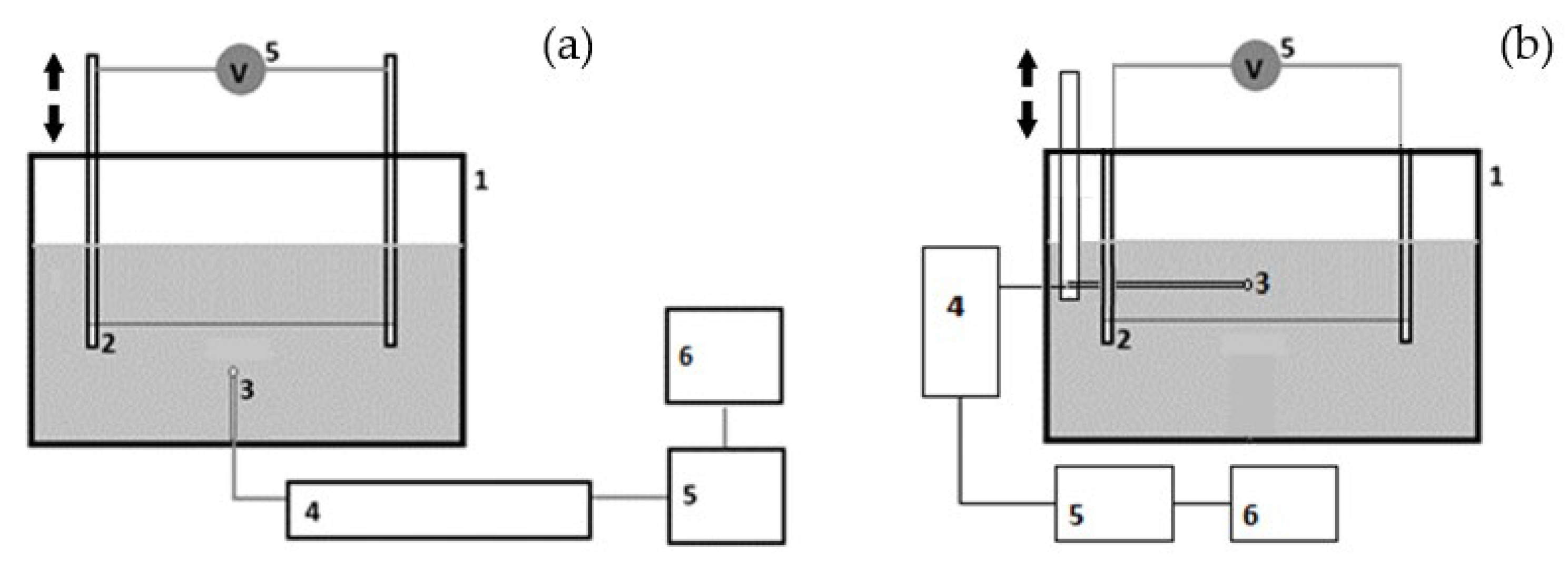
3.2. Experimental Setup and Data

Figure 5 shows the experimental setup for measuring the temperature field.

Type K thermocouple with 0.08 mm thick wire and junction’s diameter of 0.3 mm is used. The thermocouple signal is converted to a digital code with a Texas Instruments 24-bit ADC ADS1220. This ADC contains a built-in amplifier, an on-chip temperature sensor, a voltage reference, and a multiplexer. The thermocouple is connected directly to the ADC. The equalization of the crystal temperature and the cold junction temperature occurs due to the special arrangement of copper pads on adjacent layers of the printed circuit board. A microcontroller is also installed on the board, which interacts with the ADC via the serial SPI interface and transmits data via the USB interface to the computer, where the cold junction is compensated by calculation. The data are logged every 2 ms.

Two setup configurations were used in experiments: with a movable wire and a fixed thermocouple (Figure 6a) and with a fixed wire and a movable thermocouple (Figure 6b). A constantan wire with a length of 46 mm and a diameter of 0.10 mm was used, the resistance at room temperature is 2.7 ohms. The wire was energized by a power supply through a mechanical switch. For synchronization, the voltage on the wire was applied to the second channel of the ADC through optical isolation.

The container was filled with glycerol REXANT 09-3722 (99.5%). In the experiment, the heating time of the constantan wire was 30 s; afterwards, the current source was turned off. There were two cases in which the voltage drop across the wire was 0.6 V (the volumetric energy release is Q_V = 0.38 W/mm³) and 1.32 V (Q_V = 1.83 W/mm³). Thermocouple was placed at 0.6, 1.1, 1.6, 2.1, 2.6, and 3.1 mm from the axis of the wire along vertical line.

For glycerol, the Prandtl number at 25 °C Pr = 7613 [49], the Grasgoff and Rayleigh numbers for the first case of wire heating Gr ~5.3 × 10⁻⁸ and Ra ~4.0 × 10⁻⁴, for the second case Gr ~2.5 × 10⁻⁷ and Ra ~1.9 × 10⁻³. The values of these characteristic parameters make it possible to estimate the Nusselt number Nu_D for the case of stationary energy supply to the wire, defined as the ratio of convective heat flux to thermal conductivity heat flux [55,56,57,58]. According to [55], for the first heating case, the Nusselt number is minimal and is Nu_D ~0.45, for the second case Nu_D ~0.54. These numbers indicate a relatively small contribution of convection to the heat transfer process. However, it should be emphasized that the above estimates are valid only for a stationary heat source. For the non-stationary case, there is a delay of onset of convection, that has an order of 1–3 s for water [17,59], and for glycerol under heating conditions close to the first variant, the delay is tenths of a second [17].

Therefore, for the non-stationary case in our consideration, experimental verification of the effect of the possible movement of glycerol on the heat transfer process is necessary.

Figure 7 shows temperature increase for both cases with thermocouple positioned 1.1 mm above and below the wire.

The ratio of the maximum temperatures for these thermocouple positions is low for 0.6 V (0.38 W/mm³) case and high (up to 1.8 times) for 1.32 V (1.83 W/mm³) case. This means that in general the convection takes place in both cases, but in the first case, it is small. This statement is in accordance with [17], where for similar parameters of a non-stationary process, glycerol convection was not observed over a long time interval. Below, the case Q_V = 0.38 W/mm³ will be referred as “diffusion” case, and the case Q_V = 1.83 W/mm³ as “convection” case.

In case of stationary heating, the convection leads to liquid motion, and the problem should be considered in 2D formulation. For the “diffusive” case, the convection is weak or absent, and the process is close to one-dimension heat propagation by heat diffusion. However, even for the presence of the convection for considered vertical line, the derivation $\frac{\partial T}{\partial \phi }$ (φ is the angular coordinate) is zero due to the symmetry factor, and the derivation $\frac{\partial T^2}{\partial {\phi }^2}$ is negligible for the moderate heating regime in comparison with $\frac{{\partial }^{2}T}{\partial r^2}$. The main difference from the pure “diffusive” case (13) for a vertical line above the wire is the appearance of a term with velocity of the liquid on the left side of Equation (12). In addition to the idea of minimizing the data to recover the equation, this is why the experimental data were measured along a single vertical line.

Experimental data have a serially uncorrelated noise. Figure 8 shows its probability distribution calculated on 15,000 samples that is very close to the normal distribution with standard deviation of 0.024 K. Due to this reason, an additive white Gaussian noise is used in our simulations of synthetic data.

4. Results

4.1. Evolutionary Optimization Algorithm

A series of experiments were carried out to assess the performance of the proposed algorithm. Firstly, the algorithm was tested for the ability to handle the noise in the synthetic data. Basically, it could be reduced to the ability of the numerical differentiation algorithm to handle the experimental data. Secondly, the ability of the algorithm to handle the experimental data was checked as well. Lastly, the ability of the algorithm to separate “diffusion” and “convection” cases was tested.

For each experiment, the same token families $F=\{F_{diff}=\{{\left(\frac{{\partial }^{p_1+p_2}u}{\partial r^{p_1}\partial t^{p_2}}\right)}^{p_3}\}{\displaystyle \cup F_{inv}}=\{\frac{1}{r^{p_4}}\left\}\right\}$ for two-dimensional discrete grid $X=(r,t)$ were used, $u=T-T_0$. For token families, the order and power of time and spatial derivatives as $0\le p_1+p_2\le 2$ and $p_3\le 2$, respectively, are restricted, i.e., only first and second-order equations can be discovered. Additionally, inverse terms only for spatial coordinate $r$ with order restriction $0\le p_4\le 2$ are employed.

Other restrictions are the number of tokens in term $N_{tokens}\le 2$ and the number of terms as $L\le 5$. Any combinations of tokens are allowed as soon as they comply with all the restrictions, as an example $u\frac{\partial u}{\partial t}$, $\frac{1}{r}\left(\frac{{\partial }^{3}u}{\partial r\partial t^2}\right)$, $u^2$ are valid tokens.

The local approximation with polynomials is used for token precomputing. For every discrete grid point $\overline{x}=(\overline{r},\overline{t})\in X$ symmetrically, $N_{po\mathrm{int}s}$ is taken in each variable direction or ${(N_{po\mathrm{int}s})}^d$ in case of mixed partial derivative involving $d$ variables. For a given set of points $X_{fit}=\{{\overline{x}}_1,\dots ,\overline{x},\dots ,{\overline{x}}_{N_{po\mathrm{int}s}}\}$ and data values $Y_{fit}=\{u({\overline{x}}_1),\dots ,u({\overline{x}}_{N_{po\mathrm{int}s}})\}$ polynomial $P(\overline{x})$ of degree $D_{poly}$ with coefficients, $\theta$ is fitted by means of usual least square method as shown in (14).

$$\theta *=\underset{\theta }{\min }\left|\right|P(X_{fit};\theta )-Y_{fit}|{|}_2$$

(14)

In (14), polynomial computed set is a vector of polynomial values that are computed at every point ${\overline{x}}_i\in X_{fit}$, i.e., $P(X_{fit};\theta )=\left\{P\left({\overline{x}}_1;\theta \right),\dots , P\left({\overline{x}}_{N_{po\mathrm{int}s}};\theta \right)\right\}$. The derivatives are taken correspondingly for every discrete grid point as ${\frac{{\partial }^{p_1+p_2}{P}_{\overline{x}}}{\partial r^{p_1}\partial t^{p_2}}|}_{x=\overline{x}}$.

For the calculations with artificially induced noise, filtered synthetic data (13) are taken, and a Gaussian noise with distribution $N(0,\sigma )$ is applied, where $\sigma =\eta ·\max (u)$. That means that the noise is applied as a ratio of an input field maximal value is applied.

The distribution of coefficients for ten consequent runs for corresponding noise ratios is shown in

Table 1. Coefficients of Equation (15) for various noise levels.

Noise Level η, %	c1, mm2/s	c2, mm2/s	c3, K/s
0	0.154 ± 0.000	0.150 ± 0.000	0.000
0.1	0.153 ± 0.000	0.151 ± 0.000	0.000
0.3	0.14 ± 0.03	0.14 ± 0.03	0.002 ± 0.005
0.5	0.15 ± 0.2	0.15 ± 0.05	0.05 ± 0.03
0.7	0.13 ± 0.04	0.14 ± 0.07	0.10 ± 0.05
1.0	0.11 ± 0.07	0.13 ± 0.3	0.3 ± 0.1

. Agar–agar parameters were used for simulations (a_t = 0.152 mm²/s). Every value in table has the form $x\pm \mathsf{\Delta }x$, where $x$ is the mean value estimation computed over the ten runs and $\mathsf{\Delta }x$ is the 95% confidence interval computed using the corresponding normal distribution quantile. All equations were renormalized such that $\frac{\partial u}{\partial t}$ coefficient is equal to minus one. The structure that was recovered after ten runs is:

$$c_1\frac{{\partial }^{2}u}{\partial r^2}+c_2\frac{1}{r}\frac{\partial u}{\partial r}+c_3-\frac{\partial u}{\partial t}=0$$

(15)

It should be noted that spurious terms appear during the discovery procedure starting from 0.3% noise test and they are cancelled out as insignificant.

Calculations with a noise level above 1% result in an incorrect optimal equation structure. Thus, the maximum noise level is about 1%, which is considered sufficient for experimental data for the current application.

The experimental data were obtained for points along one vertical line above the wire. Due to the “one-dimensional” character of the data, the tokens do not contain an angular coordinate.

For calculations with experimental data, the filtered data are taken. The best filtering results were obtained with a fitting neural network to approximate the experimental data. For the process corresponding to the “diffusion” case, the resulting equation has the expected structure of the heat equation in cylindrical coordinates (15) with all the necessary assumptions, matching the studied problem statement. The calculated values of the coefficients are shown in

Table 2. Coefficients of Equation (15) for experimental data.

QV, W/mm3	c1 × 102, mm2/s	c2 × 102, mm2/s	c3, K/s
0.38	9.42 ± 0.04	9.40 ± 0.11	0.00 ± 0.01
1.83	9.4 ± 0.3	9.51 ± 0.27	$N(u)$

.

To find the equation for the “convection” case, the algorithm with the same parameters is employed. The convection velocity field can be taken into account as a separate token. Instead of this, there is an attempt to see how the algorithm approximated the velocity field without a separate velocity token. It is expected that there will not be a stable structure that determines the velocity field. However, the unstable remainder could thereafter be approximated with separate parametric function.

Differential tokens were obtained by approximating data with neural network training and following automated differentiation. That means that the interpolating polynomial is replaced with the fully connected dense neural network $NN(\overline{x})$ that is fitted using all grid point set $X$ as input and observation values $u$ (namely, Figure 4) as output.

In Table 2, various “noise” representations of the convection velocity field $N(u)$ are shown; for example, $N(u)=7.2\times {10}^{-7}{u}^2+3.30\times {10}^{-7}$.

The calculated values of the heat diffusion coefficient are very close to the known parameters of glycerol (a_t = 0.0926 mm²/s) for both cases. The presence of the term N[u] distinguishes modes with and without convection.

4.2. Best Subset Selection Algorithm

Four tokens were considered in the BSS algorithm as parts of the model. In addition to the terms included in the “classical” equation of thermal conductivity, written in a cylindrical coordinate system, $\frac{\partial u}{\partial t},\frac{{\partial }^{2}u}{\partial r^2},\frac{1}{r}\frac{\partial u}{\partial r}$, another term $\frac{{\partial }^{2}u}{\partial t^2}$ was added. This term is important when considering high-energy, fast-flowing thermal processes, as well as processes in small-sized objects. According to (4), the template of the equation now is

$$M_{BSS}=c_0+c_1\frac{\partial u}{\partial t}+c_2\frac{{\partial }^{2}u}{\partial t^2}+c_3\frac{{\partial }^{2}u}{\partial r^2}+c_4\frac{1}{r}\frac{\partial u}{\partial r}=0.$$

(16)

The coefficients $c_0=0$ and $c_1=-1$. The coefficient at the second time derivative $c_2$ can be identified with the relaxation time ${\tau }_r$ of the heat flux: $c_2=-{\tau }_r$. The coefficient $c_3=a_t$ ($a_t$ is the thermal diffusivity). $c_4$ is related to the cylindrical geometry of the problem. In the case of natural convection according to (12), the coefficient $c_4$ is also related to the convection motion with the velocity $v_r$. Thus, the form of the equation under study represents a wide range of thermal processes while having a substantially smaller working token count than the evolutionary optimization approach. It should be noted that in the present paper, coefficients in (16) are supposed to be constants.

The following algorithm steps correspond to the one described in Section 2.2. In the case of the noiseless initial data, the vectors Y_j, which contain finite-different (FD) templates of corresponding terms in (16), are calculated by given synthetic or experimental distributions of temperature $u$ on a spatial regular grid with step ${\tau }_s$ and temporal grid with step ${\tau }_t$. The FD approximation of $\frac{{\partial }^{2}u}{\partial t^2}$ contains three-time layers and has the second order accuracy $O({\tau }^2)$, and the FD approximation of $\frac{\partial u}{\partial t}$ is the central difference corresponded to $O({\tau }^2)$. The FD approximations with second order $O(h^2)$ are also employed for space derivatives in (16).

In the case of noisy data, the direct application of the algorithm is not successful due to errors in the numerical differentiation procedure. In the paper, the BSS algorithm is modified to work with noisy data. In contrast to data filtering procedure, described in the previous section, the proposed regularization approach is based on the choice of the step of numerical differentiation, considering the noise level [30] when calculating the components of the vectors Y_j.

The time/space steps for numerical differentiation can be estimated according to [4]:

$${\tau }_{reg,1}\approx \frac{2{\sigma }_E}{{\epsilon }_1}, {\tau }_{reg,2}\approx {\left(\frac{4{\sigma }_E}{{\epsilon }_2}\right)}^{1/2}.$$

(17)

Here, ${\epsilon }_1$ and ${\epsilon }_2$ are the absolute errors of the first and second derivatives of temperature over time/space, σ_E is the absolute error of temperature measurement. More accurate data are required when larger values of ${\tau }_{reg}$ should be used. It is assumed that the steps of numerical differentiation should be greater than ${\tau }_{reg,1}$ and ${\tau }_{reg,2}$ but much less than the characteristic process time/length.

The analysis of the effect of the noise level on the efficiency of the algorithm was carried out for synthetic data on the heating of agar-agar ($a_t$ = 0.152 mm²/s) generated with the time step of 2 ms and the space step of 10 um (

Table 3. Coefficients of Equation (16) for various noise levels.

Noise Level, %	c3, mm2/s	c4, mm2/s	c0 × 104, K/s
0	0.152 ± 0.000	0.149 ± 0.000	(−3.74 ± 0.00) × 10−2
0.1	0.153 ± 0.001	0.1556 ± 0.0018	4.36 ± 1.3
0.5	0.133 ± 0.005	0.13 ± 0.08	−5 ± 4
1.0	0.10 ± 0.05	0.09 ± 0.01	−13 ± 9
1.5	0.074 ± 0.009	0.054 ± 0.013	−12 ± 9

). In the case of the noisy data at the stage of model reconstruction, the step of numerical differentiation in the calculation of finite-difference patterns of the first and the second derivatives in time is ${\tau }_{reg,t}$ = 4 s and in space ${\tau }_{reg,s}$ = 0.5 mm. The last value corresponds to the distance between the measurement points in the experiment. The structure of the model is restored correctly when the noise level is less than 1.5%. The accuracy of the recovery coefficients decreases with an increasing noise level and for an amplitude of 0.5% is at the level of 12%.

The numerical estimation of the first and the second derivatives of temperature with respect to time for the experimental data under consideration shows that to achieve a relative error of 10% with an error in the data ${\sigma }_E$ = $\sigma$ = 0.024 K (corresponding to approximately 1% noise level), the value of the time step of numerical differentiation must be ${\tau }_{reg,t}$ ≈ 1 s or more. This value is significantly higher than the temperature measurement step in the experiment, equal to 2 ms.

The results of applying the BSS algorithm to experimental data with different granularity of numerical differentiation in time and space ${\tau }_{reg,s}$ = 0.5 mm are shown in

Table 4. Coefficients of Equation (16) for experimental data and various ${\tau }_{reg,t}$.

QV, W/mm3	τreg,t, s	c3 × 102, mm2/s	c4 × 102, mm2/s	c0 × 103, K/s
0.38	0.2	7.131	4.608	−2.095
0.38	1	6.832	4.374	−2.190
0.38	2	7.000	4.502	2.312
0.38	5	7.261	4.809	−1.863
1.83	0.2	8.818	1.354	−40.29
1.83	1	8.813	1.425	−39.90
1.83	2	8.074	-	−44.59
1.83	5	7.951	-	−44.14

. For the time granularity less than 0.2 s, the structure of the equation was not restored correctly, a term $\frac{{\partial }^{2}u}{\partial t^2}$ appears and a term $\frac{1}{r}\frac{\partial u}{\partial r}$ are absent. With decreased time granularity, the structure of the equation was restored correctly. For ${\tau }_{reg,t}$ > 0.2 s, the recovered values of the coefficients $c_3$ and $c_4$ changed slightly. For a step of 5 s, the recovery error of the coefficient c₃ with the token $\frac{{\partial }^{2}u}{\partial r^2}$, which is associated with the thermal diffusivity coefficient of glycerol ($a_t$ = 0.0926 mm²/s), turns out to be about 20% for the “diffusion” case and 12% for the case of “convection”. For the “diffusion” case, the discrepancy between the coefficients $c_3$ and $c_4$ is about 50%. Even while taking the error in determination of $c_4$ into account, such a high discrepancy may indicate the presence of a weak convection of glycerol, even in the case of low power supplied to the wire. Regarding the case of “convection”, the $c_4$ term is significantly reduced due to the presence of the medium velocity or is not restored at all. Thus, a significant difference between the coefficients can be used as an indicator of the presence of convection with pulsed heating of a viscous liquid.

4.3. Adaptive Single-Objective Optimization

To evaluate the efficiency of restoring the equation coefficients for the generated model using the proposed approaches, the inverse problem of heat conduction was solved by one of the classical methods (see Section 2.3).

The unknowns in the heat conduction equation are supposed to be the heat flux at the boundary of the wire q and the coefficient of thermal conductivity λ. Other parameters of the material are supposed to be known. The initial data for the coefficient problem are the measured values of the temperature at different distances from the wire (see Section 3.2).

The coefficient problem was solved for the constructed error functional to be minimized: $U=\underset{m,n}{\min }{\displaystyle \sum _k\left|u_{num}(q_m,{\lambda }_n,r_k,t_i{)-\mathrm{u}}_{\exp }(r_k,t_i)\right|}$, where $u_{\exp }(r_k,t_i)$ is the measured temperature increase ($u=T-T_0$) at a distance $r_k$ from the wire at the time $t_i$ and $u_{num}(q_m,{\lambda }_n,r_k,t_i)$—temperature increase, calculated from the values of $q$ and $\lambda$ according to the optimization algorithm at the same point at the same time. The algorithm requires the following settings (

Table 5. Algorithm settings.

qmin, W/m2	qmax, W/m2	λmin, W/(m × K)	λmax, W/(m × K)	NIS	MNE	CT
5000	15,000	0.1	0.5	6	20	10−6

): the initial ranges ($q_{\min },\hspace{0.17em}{q}_{\max }$) and (${\lambda }_{\min },\hspace{0.17em}{\lambda }_{\max }$), the initial number of pairs ($q,\hspace{0.17em}\lambda$) (Number of Initial Samples, NIS), the maximum number of steps (Maximum Number of Evaluations, MNE), and the error of the solution (Convergence Tolerance, CT).

The convergence of the algorithm took place for both parameters—the heat flux at the boundary of the wire $q$ and the coefficient of thermal conductivity $\lambda$. The error has been reduced to 0.12 K. In this case, the calculated values of the thermal conductivity coefficient $\lambda =$ 0.34 W/(m·K) and the heat flux $q=$ 10,800 W/m² ($Q_V=$ 0.43 W/mm³). Accordingly, the coefficient of thermal diffusivity $a_t=\lambda /(c_p\rho )=$ 0.115 mm²/s, and the difference from the reference value (0.0926 mm²/s) was about 20%. The further increase in MNE or/and CT does not change the result.

It should be noted that the used classical method does not restore the equation structure. The structure should be known a priori.

5. Discussion

Inverse problem algorithms in heat transfer are used to recover thermophysical parameters, boundary conditions, temperature distributions, and internal heat source power from available data. Traditional algorithms assume the knowledge of the equation’s structure, but the emerging approach aims to simultaneously discover the equation’s structure and coefficients through generative design methods. Recovering the equation’s structure is crucial for understanding processes, including hidden accompanying processes. However, noise poses a challenge to these algorithms.

Noise effects can be estimated through testing on synthetic data, but hidden processes can only be detected with real experimental data. The experiments on non-stationary heating of a viscous liquid using a merged heat source (wire) to test generative design algorithms have been carried out within the present work. The experimental peculiarities include:

(1)

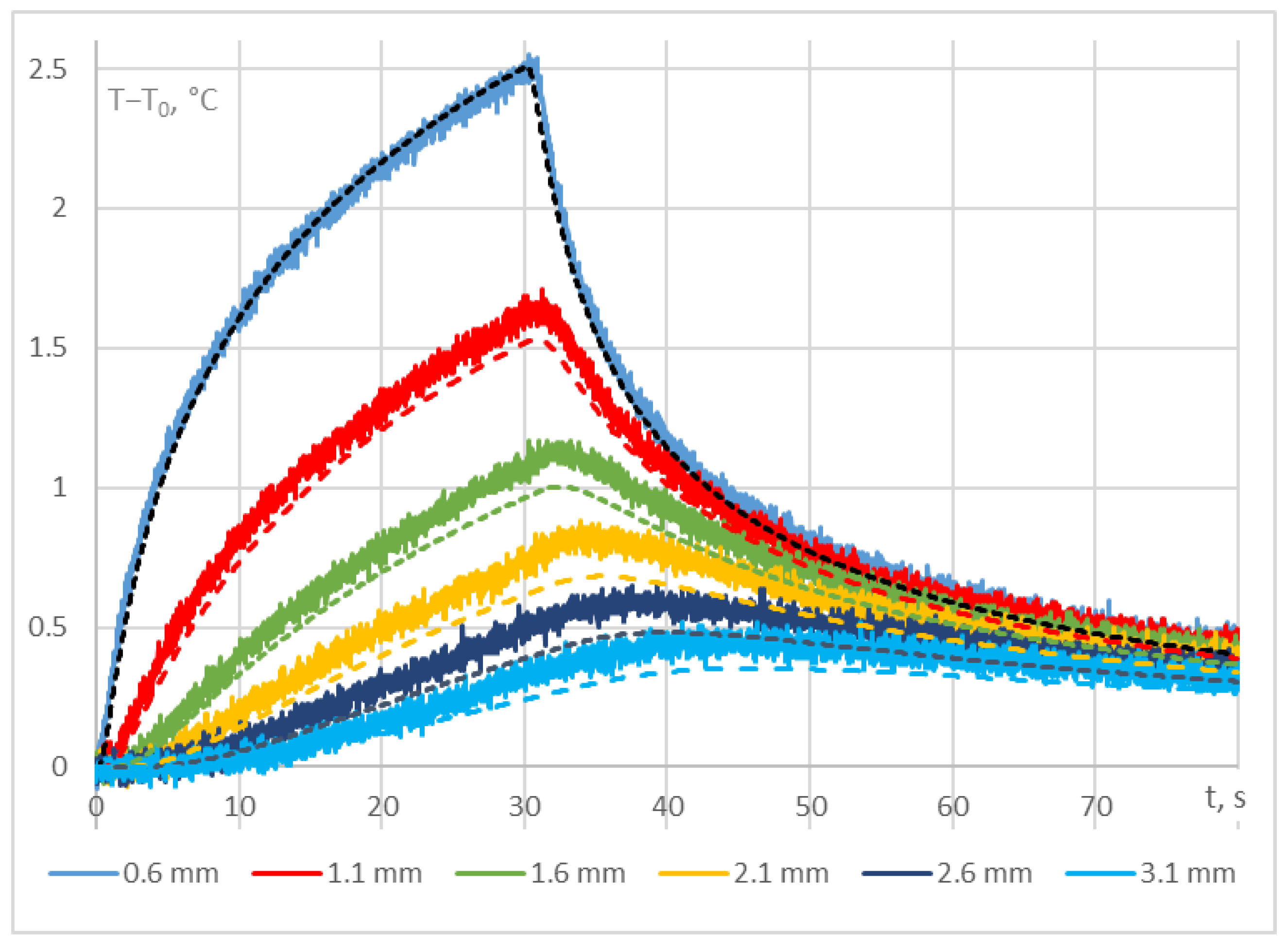
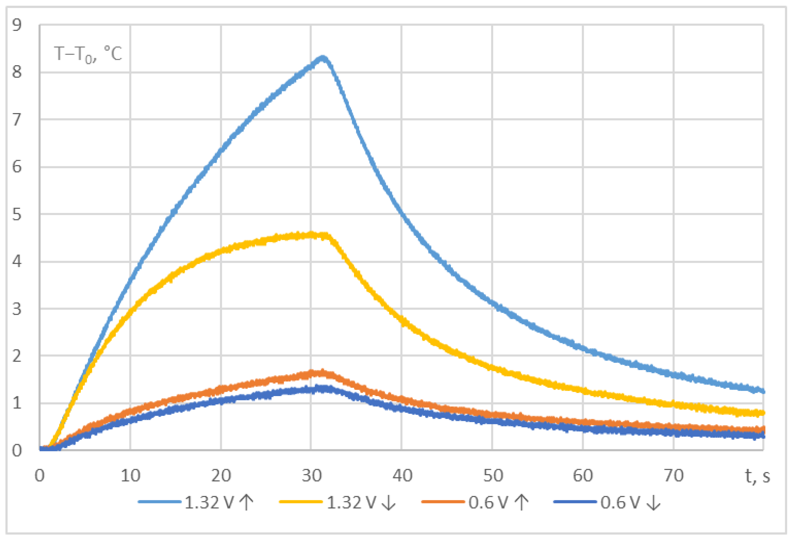
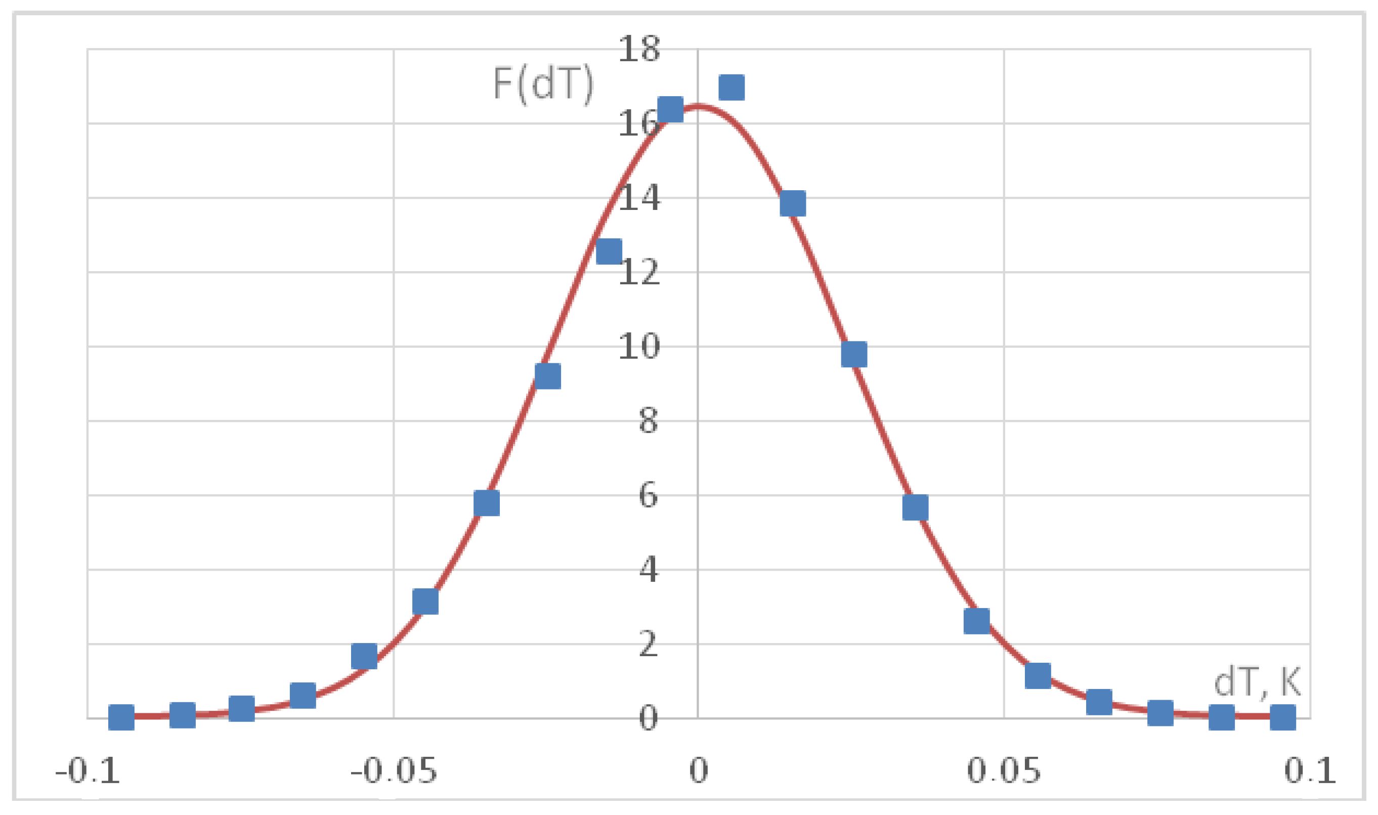
Temperature measurements in the viscous liquid (glycerol) were conducted in pulse mode. The maximum temperature observed at the nearest measurement point to the wire was approximately 2.5 °C for the first mode and around 7.5 °C for the second mode. The measurement error exhibited additive Gaussian noise with a standard deviation of 0.024 °C. Thus, the noise level was approximately 1% relative to the maximum temperature for the first case and 0.2% for the second case. The error measurement relative to the maximum observed value is more illustrative than related to the mean value used in the most papers.

(2)

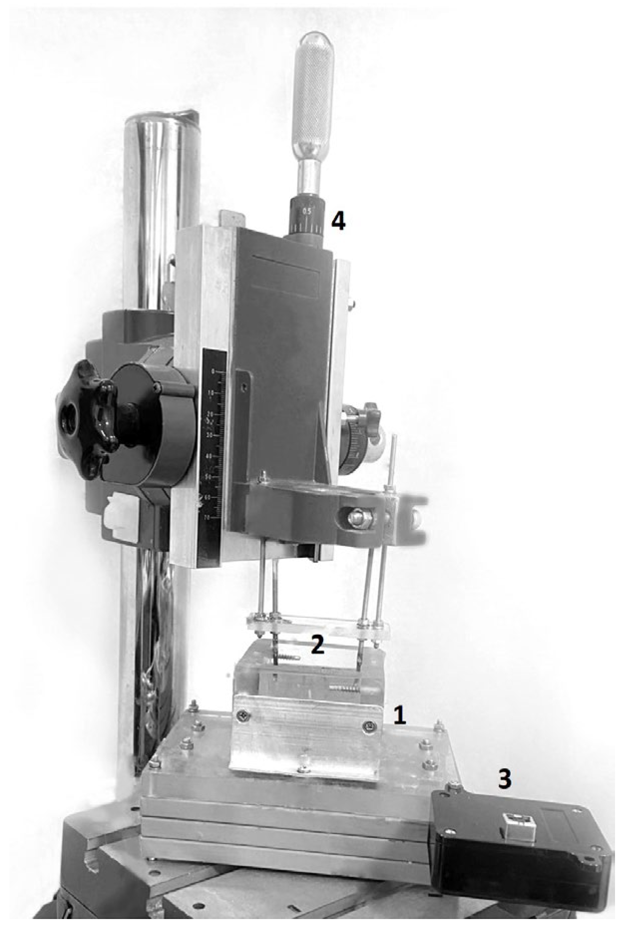
The spatial data are highly sparse. The main measurements were only taken at six points located vertically above the wire.

(3)

For the second heating mode, characterized by higher power, the conducted measurements clearly indicate the presence of convective motion in the medium.

The paper presents two approaches for recovering the model, a partial differential equation, from noisy data. Compared to the previously published works (see the Introduction section), the algorithms presented in this study enable the simultaneous recovery of both the first and the second temporal derivatives. Additionally, to accommodate the available experimental data, the algorithms have been adapted to work in a cylindrical coordinate system.

The first approach uses an evolutionary algorithm to generate the model efficiently, incorporating data smoothing and filtering with neural networks. The proposed approach demonstrates high efficiency, accurately restoring the thermal process model structure for noise levels up to 1% of the measured value’s amplitude. The coefficient error is within 30%, decreasing with decreasing noise levels. When applied to experimental data, the algorithm correctly restores the heat transfer equation’s structure and determines the thermal diffusivity coefficient with an error of 3%. In comparison, the standard adaptive single-objective optimization algorithm has a coefficient error of 20%. The algorithm can also indicate additional processes not directly measured in the experiment, as seen in the transition to developed convection.

The second algorithm is less universal and requires knowledge of the potential structure of the differential equation with the maximum number of terms. The best subset selection procedure reduces the initial terms to match the specific process, while an additional original algorithm based on choosing appropriate temporal and spatial steps mitigates the noise influence. For synthetic data, this algorithm’s efficiency is comparable to the evolutionary algorithm. In processing experimental data, the algorithm can correctly restore the model structure, but the error in determining the thermal diffusivity coefficient is within 20%, worse than the evolutionary algorithm. It should be emphasized that the above-mentioned error is achieved with very sparse data (6 spatial points and 16 temporal layers with a numerical differentiation step of 5 s). The optimal subset selection algorithm can also indicate accompanying processes.

Both algorithms predict convective motion in glycerol for significant wire heating power, consistent with observations. The evolutionary optimization algorithm introduces additional terms in the model structure, while the best subset selection algorithm reduces the restored coefficient value for the first spatial derivative. For weak heating, the experimental data do not provide a definitive conclusion about the onset of convection, with the evolutionary algorithm predicting its absence and the best subset selection algorithm suggesting weak convection. Further testing on various experimental data is necessary to indicate low-intensity processes accurately.

6. Conclusions

The aim of the study is to adapt methods of partial differential equation discovery to work with real experimental data. The results obtained may be summarized as:

(1)

two algorithms for processing sparse and noisy data are proposed, based on (i) data filtering and subsequent interpolation in the entire domain using a neural network, and (ii) selection of space and time steps within the procedure of data numerical differentiation;

(2)

the algorithms are implemented in two methods for recovering equations based on (i) a genetic algorithm with evolutionary optimization and (ii) the best subset selection procedure that showcases the capabilities of established sparse regression methods;

(3)

to verify the methods, an experiment was carried out on pulsed heating of a viscous liquid by a submerged heat source; natural noisy data on temperature changes at only six spatial points were obtained;

(4)

for the first time, on the same experimental data, the efficiency of the genetic algorithm, the best subset selection procedure, and the standard adaptive single-objective optimization algorithm of the Ansys package have been compared. The genetic algorithm and BSS procedure made it possible to correctly restore the structure of the equation in the polar coordinate system and to determine the thermal diffusivity coefficient for a noise level of up to 1% of the amplitude temperature value. The ASO algorithm, firstly, assumes prior knowledge of equation structure, and secondly, the accuracy of reconstructing the thermal diffusivity turns out to be slightly worse in relation to the results of applying the genetic algorithm;

(5)

for the first time, the possibility of indicating the process of convection of a viscous liquid using methods for reconstructing an equation in the form of a PDE was analyzed for highly sparse temperature data obtained for points along only one straight line. The proposed approach can be used to determine the onset of convection when studying the natural convection of liquids;

(6)

the capacity of methods for the discovery of equations containing higher-order time derivatives has been extended.

The use of methods based on genetic algorithms, sparse regression methods, the BSS procedure with statistical criteria is a new trend for studying real heat transfer problems. The obtained data on the effectiveness of their application on experimental data are extremely important for understanding the possibilities and limitations of the considered methods.

References

1. Tarantola, A. Inverse Problem Theory and Methods for Model Parameter Estimation; SIAM: Philadelphia, PA, USA, 2005. [Google Scholar] [CrossRef]
2. Kirsch, A. An Introduction to the Mathematical Theory of Inverse Problems, 2nd ed.; Springer: New York, NY, USA, 2013; 310p. [Google Scholar] [CrossRef]
3. Beck, J.V.; Blackwell, B.F.; St. Clair, C.R. Inverse Heat Conduction: Ill-Posed Problems; John Wiley & Sons Ltd.: Chichester, UK, 1985. [Google Scholar]
4. Vatulyan, A.O. Inverse Coefficient Problems in Mechanics; Fizmatlit: Moscow, Russia, 2019; 272p. (In Russian) [Google Scholar]
5. Yang, J.P.; Li, H.-M. Recovering Heat Source from Fourth-Order Inverse Problems by Weighted Gradient Collocation. Mathematics 2022, 10, 241. [Google Scholar] [CrossRef]
6. Maslyaev, M.; Hvatov, A.; Kalyuzhnaya, A. Discovery of the data-driven models of continuous metocean process in form of nonlinear ordinary differential equations. Procedia Comput. Sci. 2020, 178, 18–26. [Google Scholar] [CrossRef]
7. Somacal, A.; Barrera, Y.; Boechi, L.; Jonckheere, M.; Lefieux, V.; Picard, D.; Smucler, E. Uncovering differential equations from data with hidden variables. arXiv 2020, arXiv:2002.02250v2. [Google Scholar] [CrossRef] [PubMed]
8. Chen, Z.; Liu, Y.; Sun, H. Physics-informed learning of governing equations from scarce data. Nat. Commun. 2021, 12, 6136. [Google Scholar] [CrossRef]
9. Bykov, N.Y.; Obraztsov, N.V.; Hvatov, A.A.; Maslyaev, M.A.; Surov, A.V. Hybrid modeling of gas-dynamic processes in AC plasma torches. Mater. Phys. Mec. 2022, 50, 287–303. [Google Scholar] [CrossRef]
10. Xu, H.; Zeng, J.; Zhang, D. Discovery of Partial Differential Equations from Highly Noisy and Sparse Data with Physics-Informed Information Criterion. Research 2023, 6, 0147. [Google Scholar] [CrossRef] [PubMed]
11. Schmidt, M.; Lipson, H. Distilling free-form natural laws from experimental data. Science 2009, 324, 81–85. [Google Scholar] [CrossRef]
12. Li, W.; Dong, Y.; Wang, J.; Zhang, Y.; Zhang, X.; Liu, X. Experimental study on enhanced heat transfer of nanocomposite phase change materials. Phase Transit. 2019, 92, 285–301. [Google Scholar] [CrossRef]
13. Zhang, Y.; Du, K.; Medina, M.A.; He, J. An experimental method for validating transient heat transfer mathematical models used for phase change materials (PCMs) calculations. Phase Transit. 2014, 87, 541–558. [Google Scholar] [CrossRef]
14. Rathod, M.K.; Banerjee, J. Experimental Investigations on Latent Heat Storage Unit using Paraffin Wax as Phase Change Material. Exp. Heat Transf. 2014, 27, 40–55. [Google Scholar] [CrossRef]
15. Duluc, M.-C.; Xin, S.; Le Quéré, P. Transient natural convection and conjugate transients around a line heat source. Int. J. Heat Mass Transf. 2003, 46, 341–354. [Google Scholar] [CrossRef]
16. Duluc, M.-C.; Xin, S.; Lusseyran, F.; Le Quéré, P. Numerical and experimental investigation of laminar free convection around a thin wire: Long time scalings and assessment of numerical approach. Int. J. Heat Fluid Flow 2008, 29, 1125–1138. [Google Scholar] [CrossRef]
17. Manukhin, B.G.; Gusev, M.E.; Kucher, D.A.; Chivilikhin, S.A.; Andreeva, O.V. Optical diagnostics of the process of free liquid convection. Opt. Spectrosc. 2015, 119, 392–397. [Google Scholar] [CrossRef]
18. Duluc, M.-C.; Fraigneau, Y.C. Effect of frequency on natural convection flows induced by a pulsating line-heat source. Int. J. Therm. Sci. 2017, 117, 342–357. [Google Scholar] [CrossRef]
19. Jiang, Y.; Nie, B.; Zhao, Y.; Carmeliet, J.; Xu, F. Scaling of buoyancy-driven flows on a horizontal plate subject to a ramp heating of a finite time. Int. J. Heat Mass Transf. 2021, 171, 121061. [Google Scholar] [CrossRef]
20. Samarskii, A.A.; Vabishchevich, P.N. Computational Heat Transfer, Volume 1: Mathematical Modelling, 1st ed.; John Wiley & Sons Ltd.: Chichester, UK, 1995. [Google Scholar]
21. Cattaneo, C.; Kampé de Fériet, J. Sur une Forme de L’équation de la Chaleur Eliminant le Paradoxe D’une Propagation Instantanée. Comptes Rendus Hebdomadaires des Séances de L’academie des Sciences; Gauthier-Villars: Paris, France, 1958; pp. 431–433. [Google Scholar]
22. Zhmakin, A.I. Heat Conduction Beyond the Fourier Law. Tech. Phys. 2021, 66, 1–22. [Google Scholar] [CrossRef]
23. Cai, S.; Wang, Z.; Wang, S.; Perdikaris, P.; Karniadakis, G.E. Physics-informed neural networks for heat transfer problems. J. Heat Transf. 2021, 143, 060801. [Google Scholar] [CrossRef]
24. Zhang, Q.; Guo, X.; Chen, X.; Xu, C.; Liu, J. PINN-FFHT: A physics-informed neural network for solving fluid flow and heat transfer problems without simulation data. Int. J. Mod. Phys. C 2022, 33, 2250166. [Google Scholar] [CrossRef]
25. Oommen, V.; Srinivasan, B. Solving inverse heat transfer problems without surrogate models: A fast, data-sparse, physics informed neural network approach. J. Comput. Inf. Sci. Eng. 2022, 22, 041012. [Google Scholar] [CrossRef]
26. Cai, S.; Wang, Z.; Chryssostomidis, C.; Karniadakis, G.E. Heat transfer prediction with unknown thermal boundary conditions using physics-informed neural networks. Fluids Eng. Div. Summer Meet. 2020, 83730, V003T05A054. [Google Scholar] [CrossRef]
27. Jin, G.; Xing, H.; Zhang, R.; Guo, Z.; Liu, J. Data-driven discovery of governing equations for transient heat transfer analysis. Comput. Geosci. 2022, 26, 613–631. [Google Scholar] [CrossRef]
28. Fasel, U.; Kutz, J.N.; Brunton, B.W.; Brunton, S.L. Ensemble-SINDy: Robust sparse model discovery in the low-data, high-noise limit, with active learning and control. Proc. R. Soc. A Math. Phys. Eng. Sci. 2022, 478, 20210904. [Google Scholar] [CrossRef]
29. Rudy, S.H.; Brunton, S.L.; Proctor, J.L.; Kutz, J.N. Data driven discovery of partial differential equations. Sci. Adv. 2017, 3, e1602614. [Google Scholar] [CrossRef] [PubMed]
30. Schaeffer, H. Learning partial differential equations via data discovery and sparse optimization. Proc. R. Soc. A 2017, 473, 20160446. [Google Scholar] [CrossRef] [PubMed]
31. Dal Santo, N.; Deparis, S.; Pegolotti, L. Data driven approximation of parametrized PDEs by reduced basis and neural networks. J. Comput. Phys. 2020, 416, 109550. [Google Scholar] [CrossRef]
32. Maslyaev, M.; Hvatov, A.; Kalyuzhnaya, A.V. Partial differential equations discovery with EPDE framework: Application for real and synthetic data. J. Comput. Sci. 2021, 53, 101345. [Google Scholar] [CrossRef]
33. Xu, H.; Zhang, D. Robust discovery of partial differential equations in complex situations. Phys. Rev. Res. 2021, 3, 033270. [Google Scholar] [CrossRef]
34. Xu, H.; Chang, H.; Zhang, D. DLGA-PDE: Discovery of PDEs with incomplete candidate library via combination of deep learning and genetic algorithm. J. Comput. Phys. 2020, 418, 109584. [Google Scholar] [CrossRef]
35. Bykov, N.Y.; Hvatov, A.A.; Kalyuzhnaya, A.V.; Boukhanovsky, A.V. A method for reconstructing models of heat and mass transfer from the spatio-temporal distribution of parameters. Tech. Phys. Lett. 2022, 48, 50–54. [Google Scholar] [CrossRef]
36. Hastie, T.; Tibshirani, R.; Friedman, J. The Elements of Statistical Learning, 2nd ed.; Springer: New York, NY, USA, 2009; 745p. [Google Scholar] [CrossRef]
37. R Core Team. R: A Language and Environment for Statistical Computing; R Foundation for Statistical Computing: Vienna, Austria, 2020; Available online: https://www.r-project.org/ (accessed on 6 September 2023).
38. Carslaw, H.S.; Jaeger, J.C. Conduction of Heat in Solids, 2nd ed.; Oxford University Press: Oxford, UK, 1959; 414p. [Google Scholar]
39. Sun, S.; Li, S.; Shaheen, S.; Arain, M.B.; Usman; Khan, K.A. A numerical investigation of bio-convective electrically conducting water-based nanofluid flow on the porous plate with variable wall temperature. Numer. Heat Transf. Part A Appl. 2023, 1–15. [Google Scholar] [CrossRef]
40. Bao, H.-X.; Arain, M.B.; Shaheen, S.; Khan, H.I.; Usman; Inc, M.; Yao, S.-W. Boundary-layer flow of heat and mass for Tiwari-Das nanofluid model over a flat plate with variable wall temperature. Therm. Sci. 2022, 26, 39–47. [Google Scholar] [CrossRef]
41. Bykov, N.Y. Reconstructing the thermal process model using the time-space distributions of temperature. St. Petersburg Polytech. Univ. J.-Phys. Math. 2022, 15, 83–99. [Google Scholar] [CrossRef]
42. Bykov, N.Y.; Hvatov, A.A.; Kalyuzhnaya, A.V.; Boukhanovsky, A.V. A method of generative model design based on irregular data in application to heat transfer problems. J. Phys. Conf. Ser. 2021, 1959, 012012. [Google Scholar] [CrossRef]
43. Stephany, R.; Earls, C. PDE-READ: Human-readable partial differential equation discovery using deep learning. Neural Netw. 2020, 154, 360–382. [Google Scholar] [CrossRef]
44. James, G.; Witten, D.; Hastie, T.; Tibshirani, R. An Introduction to Statistical Learning: With Applications in R, 1st ed.; Springer: New York, NY, USA, 2013; 426p. [Google Scholar] [CrossRef]
45. Priestley, M.B. Spectral Analysis and Time Series (Probability and Mathematical Statistics); Academic Press: Cambridge, UK, 1981; 890p. [Google Scholar]
46. Rathore, K.R.; Sharma, K.; Sarda, A. An Adaptive Approach for Single Objective Optimization. Int. J. Eng. Res. App. 2014, 4, 737–747. [Google Scholar]
47. Haryanto, I.; Raharjo, F.A.; Kurdi, O.; Haryadi, G.D.; Santosa, S.P.; Gunawan, L. Optimization of Bus Body Frame Structure for Weight Minimizing with Constraint of Natural Frequency using Adaptive Single-Objective Method. Int. J. Sustain. Transp. Technol. 2018, 1, 9–14. [Google Scholar] [CrossRef]
48. Li, H.; Han, Y.; Shi, W.; Tiganik, T.; Zhou, L. Automatic optimization of centrifugal pump based on adaptive single-objective algorithm and computational fluid dynamics. Eng. Appl. Comput. Fluid Mech. 2022, 16, 2222–2242. [Google Scholar] [CrossRef]
49. Animasaun, I.L.; Shah, N.A.; Wakif, A.; Mahanthesh, B.; Sivaraj, R.; Koriko, O.K. Ratio of Momentum Diffusivity to Thermal Diffusivity: Introduction, Meta-Analysis, and Scrutinization; Chapman and Hall/CRC: New York, NY, USA, 2022; 410p. [Google Scholar] [CrossRef]
50. Munafò, C.F.; Palumbo, A.; Versaci, M. An Inhomogeneous Model for Laser Welding of Industrial Interest. Mathematics 2023, 11, 3357. [Google Scholar] [CrossRef]
51. Larikov, L.N.; Yurchenko, Y.F. Thermal Properties of Metals and Alloys; Naukova Dumka: Kyiv, Ukraine, 1985; 438p. [Google Scholar]
52. Zhang, M.; Che, Z.; Chen, J.; Zhao, H.; Yang, L.; Zhong, Z.; Lu, J. Experimental Determination of Thermal Conductivity of Water−Agar Gel at Different Concentrations and Temperatures. J. Chem. Eng. Data 2011, 56, 859–864. [Google Scholar] [CrossRef]
53. Vargaftik, N.B. Handbook of Physical Properties of Liquids and Gases, 2nd ed.; Springer: Berlin/Heidelberg, Germany, 1975; 758p. [Google Scholar]
54. Rabinovich, V.A.; Khavin, Z.Y. The Concise Chemical Handbook, 2nd ed.; Khimiya: Leningrad, Russia, 1978; 392p, Available online: http://www.vixri.ru/d2/KRATKIJ%20XIMIChESKIJ%20SPRAVOChNIK.pdf (accessed on 6 September 2023). (In Russian)
55. Kutateladze, S.S. Fundamentals of Heat Transfer; Adademic Press, Inc.: New York, NY, USA, 1963. [Google Scholar]
56. Boetcher, S.K.S. Natural Convection from Circular Cylinders; Springer: Cham, Switzerland, 2014; 48p. [Google Scholar] [CrossRef]
57. Dai, C.; Wang, J. External natural convection from a Joule heated horizontal platinum wire in water at low Rayleigh number. Int. J. Heat Mass Transf. 2016, 93, 754–759. [Google Scholar] [CrossRef]
58. Cieśliński, J.T.; Smolen, S.; Sawicka, D. Free Convection Heat Transfer from Horizontal Cylinders. Energies 2021, 14, 559. [Google Scholar] [CrossRef]
59. Watanabe, H. Further examination of the transient hot-wire method for the simultaneous measurement of thermal conductivity and thermal diffusivity. Metrologia 2002, 39, 65–81. [Google Scholar] [CrossRef]
Figure 1. Cross-over scheme. Two children equations (on the right) are generated by exchanging terms in two existing parent equations (on the left).
Processes 11 02719 g001
Figure 2. Mutation scheme. There are two possibilities to obtain children: (a) through a randomly generated term exchange and (b) through a randomly generated token exchange.
Processes 11 02719 g002
Figure 3. Temperature vs. radius in glycerol for the time points t = 15 s, t = t0 = 30 s, and t = 45 s.
Processes 11 02719 g003
Figure 4. Evolution of temperature at points 0.6, 1.1, 1.6, 2.1, 2.6, and 3.1 mm from the axis. Synthetic (dashed lines) and experimental (noisy line) data (QV = 0.38 W/mm3) for glycerol medium.
Processes 11 02719 g004
Figure 5. Experimental setup. 1—container with installed thermocouple, 2—wire, 3—conversion board, 4—positioning system.
Processes 11 02719 g005
Figure 6. Experimental setup with movable wire (a) and thermocouple (b): 1—container, 2—wire, 3—thermocouple, 4—conversion board, 5—power supply, 6—PC.
Processes 11 02719 g006
Figure 7. Temperature increase vs. time for thermocouple positioned 1.1 mm above (↑) and below (↓) the wire.
Processes 11 02719 g007
Figure 8. Noise sample probability distribution (dots) and the normal distribution (curve).
Processes 11 02719 g008