Abstract
The heat transfer assessment of a buried hot oil pipe is essential for the economical and safe transportation of the pipeline, where the basis is to determine the temperature field surrounding the pipe quickly. This work proposes a novel method to efficiently predict the temperature field surrounding a hot oil pipe, which combines the proper orthogonal decomposition (POD) method and the backpropagation (BP) neural network, named the POD-BP model. Specifically, the BP neural network is used to establish the mapping relationship between spectrum coefficients and the preset parameters of the sample. Compared with the classical POD reduced-order model, the POD-BP model avoids solving the system of reduced-order governing equations with spectrum coefficients as variables, thus improving the prediction speed. Another advantage is that it is easy to implement and does not require tremendous mathematical derivation of reduced-order governing equations. The POD-BP model is then used to predict the temperature field surrounding the hot oil pipe, and the sample matrix is obtained from the numerical results using the finite volume method (FVM). In validation cases, both steady and unsteady states are investigated, and multiple boundary conditions, thermal properties, and even geometry parameters (different buried depths and pipe diameters) are tested. The mean errors of steady and unsteady cases are 0.845~3.052% and 0.133~1.439%, respectively. Appealingly, almost no time, around 0.008 s, is consumed in predicting unsteady situations using the proposed POD-BP model, while the FVM requires a computational time of 70 s.
1. Introduction
In 2022, oil accounted for the largest proportion of global energy consumption, approximately 31% [1]. Pipeline buried under the surface of the ground is the main method of transporting oil; e.g., pipeline transportation occupies 68% of domestic petroleum shipments in the United States [2]. If the oil has a high pour point or high viscosity, it should be heated to reduce friction loss and ensure the reliability of pipe transportation [3,4]. The continuous heat exchange between oil and the surrounding soil lowers the oil temperature, but the oil temperature is supposed to be kept higher than the gel point at all times during transportation, leading to great energy consumption and carbon emission from the oil heating. Therefore, efficient and accurate prediction of the temperature field around the hot oil pipe has important implications for the economical, safe, and environmentally friendly operation of the pipeline system.
In recent years, much numerical research has been carried out to investigate the temperature field surrounding the hot oil pipe, mostly based on direct numerical simulation [5], such as the finite element method (FEM) [6] and finite volume method (FVM) [7,8]. Nevertheless, direct numerical simulation has high computational complexity when solving discretization systems, resulting in large memory requirements and a long computational time. These defects make it difficult to apply to optimal design and risk assessment of the pipeline system, which requires the calculation of different conditions containing a great number of combinations of operation and structure parameters [9]. Herein, this work tends to adopt the proper orthogonal decomposition (POD) method to improve the simulation efficiency [10].
POD can abstract large amounts of data about one mathematical model into a series of basis functions to represent the main characteristics of this model [11,12]. It is always combined with the Galerkin projection method to construct the POD reduced-order model that can predict the physical field distribution [13]. The spectrum coefficients system with lower degrees of freedom is solved in the POD reduced-order model [14], rather than all discretized grids, as in direct numerical simulation, and thus the POD reduced-order model can significantly improve the simulation speed. Researchers have paid extensive attention to the POD reduced-order model, and it is widely applied to various engineering projects, including turbulent flow [15,16], and pipe flow [17]. Recently, some applications of the POD reduced-order model to predict the temperature field surrounding the hot oil pipe have been published. Yu et al. [18] established the POD reduced-order model for the pipe cross section based on the unstructured grid, in which comprehensive boundary conditions of the physical domain were considered, and the boundary treatments in the POD reduced-order model were discussed in detail. To make the POD reduced-order model suitable for different geometry parameters (i.e., buried depth, pipe diameter, and pipe wall thickness), the body-fitted coordinates (BFCs) of the pipe cross section were combined with the POD reduced-order model in [19]. This model effectively expanded the application scope of POD, but only a steady situation was studied. Furthermore, Han et al. [20] proposed a BFC-based POD reduced-order model for the unsteady heat conduction of crude oil pipelines and applied it to the cold and hot oil batch transportation as well as pipe shutdown.
The classical POD reduced-order model requires many numerical simulation results to extract the basis functions, which are then used for predicting the temperature field. However, this approach has two drawbacks: (1) There is a mapping relationship between spectrum coefficients and preset parameters of the predicted sample, described by reduced-order governing equations [20]; solving reduced-order governing equations with spectrum coefficients as variables still needs a certain amount of computation. (2) The Galerkin projection method used to derive the reduced-order governing equations from the POD basis functions requires high mathematical complexity and is tedious to implement [21]; if the assumptions underlying the heat transfer processes, such as steady or unsteady states, constant or variable thermal properties, and boundary conditions, are changed, the reduced-order governing equations must be rederived [18].
In another way, using neural networks to fit mapping relationships has high flexibility and adaptability [22,23]. The training process of neural networks does not require any complex mathematical derivation, and the application of neural networks has almost no computational effort. Hence, to address the two drawbacks of the classical POD reduced-order model mentioned above, this work uses the backpropagation (BP) neural network to establish the mapping between spectrum coefficients and preset parameters of the sample. The present model is named the POD-BP model, and it can efficiently predict the temperature field surrounding the hot oil pipe in both steady and unsteady situations. A variety of boundary, thermal property, and geometry parameters are also considered in validation cases to illustrate the applicability of the POD-BP model.
2. Methodology
This section first presents the physical model and governing equations for the temperature field surrounding the hot oil pipe. Then, the meshing of the computational domain is introduced to ensure that the POD-BP model applies to various geometry parameters. Subsequently, the POD basis function calculation is briefly described and the POD-BP model is established to predict the temperature field.
2.1. Physical Model for Heat Conduction Surrounding the Hot Oil Pipe
Figure 1 shows the schematic of the computational domain and boundary conditions for the heat conduction surrounding the hot oil pipeline. The deposited wax, steel layer, and corrosion protection layer are considered for the pipe wall, and the surrounding soil accounts for the primary area. The following assumptions are made to simplify this problem.
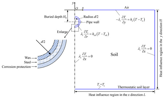
Figure 1.
Computational domain and boundary condition.
- The thermal properties of the soil and pipe wall are isotropy and homogeneous. Hence, the physical problem is symmetry along the vertical centerline of the pipe, and only half of the domain is investigated here.
- The axial temperature variation of the surrounding soil is slight compared with the radial direction and is thus neglected. A two-dimensional pipeline cross section is studied here.
- The temperatures of hot oil inside the pipe and atmosphere air and the thickness of wax deposition remain unchanged with time.
- According to the literature and engineering applications, the thermal influence regions in the x and y directions are both 10 m [5]. It is assumed that the temperature response outside the thermal influence region is neglected.
The governing equations of heat conduction in the pipe wall and surrounding soil are expressed as follows:
where T is the temperature in the physical domain; t is the time; ρ is the density; cp is the specific heat capacity; λ is the thermal conductivity; and subscripts 1, 2, 3, and s denote the wax layer, steel layer, corrosion protection layer, and soil, respectively.
For the boundary conditions, the left boundary (except the wax layer boundary) is subjected to the symmetrical boundary condition as follows:
where H0 is the buried depth; d is the inner diameter of the steel pipe; and is the thickness of the wax layer. The wax layer boundary and upper boundary are subjected to the convection boundary condition:
where Ta is the atmosphere temperature; ha is the heat transfer coefficient between the soil and air; Toil is the hot oil temperature inside the pipe; and hoil is the heat transfer coefficient between the oil and the wax layer. The right boundary is assigned as the adiabatic boundary and the lower boundary is regarded as the thermostatic soil layer and maintained at a constant value:
where Tc is the temperature of the thermostatic layer.
2.2. Meshing of the Computational Domain
Figure 2 presents the mesh of the computational domain. All areas tend to use the structured grid division. The geometry parameters of the computational domain, such as buried depth, wall thickness, and pipe diameter, might change in different samples. It is worth noting that the number of grids at the specific boundary is fixed even if geometry parameters are changed. This limitation can ensure that the connection relationship for grid cells is unchanged, even though the geometry parameters are different. Hence, the POD basis functions discussed below apply to the various geometry structures of the computational domain.

Figure 2.
Mesh of the computational domain.
Specifically, the total number of grid cells is 3846, and the upper, lower, and right boundaries have 53, 53, and 68 grids, respectively, as presented in Figure 2. The left-upper, wax layer, and left-lower boundaries have 12, 14, and 42 grids, respectively. The wax, steel, corrosion protection, and virtual soil layers each have two grids for the pipe wall. The virtual soil layer is the meshing transition from the pipe wall to the soil, and its thermal properties are the same as the soil.
2.3. Calculation of the POD Basis Functions
POD can extract the characteristic information of the physical problem through its basis functions [24]. The POD basis functions are derived from the accurate results of multiple sampling conditions, which are calculated by the finite volume method (FVM) in this work [25]. The calculation of POD basis functions may need a large amount of computation, but it is a one-off effort.
Suppose the computational domain has N grid cells, the matrix of a single sample for the steady situation or unsteady situation with K recorded moments is constructed, as shown in Equation (7). The temperature values of all grid cells and moments in a certain sampling condition are saved in the same matrix, marked as Q.
where τ is the simulation time step and Q is generated by FVM simulations. Furthermore, POD always applies to investigate various conditions, thus the Q of various sampling conditions should be assembled into the same matrix S to superimpose the influences of various conditions. It can be derived from Equation (7) that the matrix Q for the steady situation has only one column to describe one steady temperature field, while for the unsteady situation with K recorded moments, the matrix Q consists of K columns to describe multiple temperature fields. Considering that there are L kinds of sampling conditions, an entire sample matrix is constructed:
The basis functions are obtained by applying the singular-value decomposition method [26] to S. When the row number Nr of S is smaller than its column number Nc, the basis functions are calculated by the following steps:
- Calculate the matrix ;
- Orthogonally decompose the matrix and obtain a series of eigenvectors wi (i = 1, 2, 3, …, Nr). Sort eigenvectors wi by their corresponding eigenvalues.
- The basis functions are ;
- If Nr is larger than Nc, the following steps are conducted:
- Calculate the matrix ;
- Orthogonally decompose the matrix and obtain a series of eigenvectors wi (i = 1, 2, 3, …, Nc). Sort eigenvectors wi by their corresponding eigenvalues.
- The basis functions are ;
- In general, the matrix of basis functions is expressed as follows:
The POD basis functions can be arranged in descending order of eigenvalues, which represents the energy or necessities of each basis function. The front POD basis functions possess the most energy and are selected to characterize the physical problem. If the first M basis functions were used to approximately construct the temperature field, the original sequence is rewritten as follows:
2.4. Establishment of the POD-BP Prediction Model
In the classical POD reduced-order model, the spectrum coefficients are solved by the reduced-order governing equations when the basis functions are attempted to represent the predicted sample. In other words, there is a mapping between the predicted sample and its related spectrum coefficients, described by the reduced-order governing equations in the classical POD reduced-order method. However, the BP neural network substitutes the reduced-order governing equations to establish the mapping in this work. The following firstly introduces the construction of the dataset for the neural network, and then the entire calculation process of the POD-BP model is presented.
After obtaining the sample matrix and the POD basis functions, we can construct the spectrum coefficient matrix as the target data of the BP neural network. It is computed by the projection of the sample matrix to the basis functions matrix:
where every column of A is regarded as a set of outputs of neural networks.
On the other hand, the input data of the BP neural network are derived from the preset parameters of samples, including boundary parameters, thermal property parameters, geometry parameters, and the simulation time step if there is an unsteady situation. It is apparent that, for all samples, the preset parameters and the associated output spectrum coefficients have a mapping and form a dataset. Then, a typical BP neural network [27,28], which usually has a two-layer feed-forward framework, sigmoid hidden neurons, and linear output neurons, is established, as shown in Figure 3. For the training process of the BP neural network, the dataset is split into training, validation, and testing sets in a ratio of 7:1.5:1.5, and the Levenberg–Marquardt algorithm is implemented [29,30].
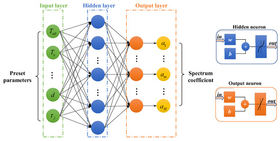
Figure 3.
The BP neural network used to predict the spectrum coefficients through the input of preset parameters of the sample.
The predicted spectrum coefficients of the BP neural network can be used to reconstruct the temperature field by substituting them into Equation (12). The entire calculation process of the POD-BP model is presented in Figure 4.
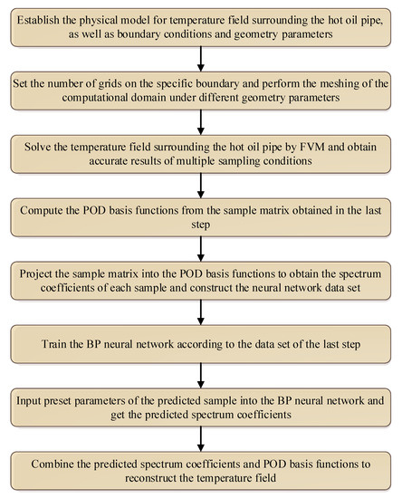
Figure 4.
The entire calculation process of the POD-BP model to predict the temperature field surrounding the hot oil pipe.
3. Results and Discussion
This section employs the POD-BP model to predict the soil temperature field for both steady and unsteady situations. The accuracy of the prediction results is testified by comparing them with the results of FVM.
First, the parameters, which are constant for all sampling conditions, are given. The wax layer, steel layer, corrosion protection layer, and virtual soil layer thicknesses are fixed at 0.016 m, 0.02 m, 0.005 m, and 0.02 m, respectively. The specific heat capacities of wax, steel, corrosion protection, and soil are 2100 J·kg−1·°C−1, 465 J·kg−1·°C−1, 1670 J·kg−1·°C−1, and 1010 J·kg−1·°C−1, respectively, and their densities are 910 kg·m−3, 7800 kg·m−3, 1200 kg·m−3, and 1700 kg·m−3, respectively. The thermal conductivities of wax, steel, and corrosion protection are 2.5 W·m−1·°C−1, 48.0 W·m−1·°C−1, and 0.15 W·m−1·°C−1, respectively. For the boundary parameters, the convective heat transfer coefficients of oil and atmosphere are fixed at 100 W·m−2·°C−1 and 20 W·m−2·°C−1, respectively.
Table 1 and Table 2 list the sampling conditions, which are also the preset parameters of samples. They are solved by FVM with an algebraic multigrid solver, and the results are used to form the sample matrix. There are three boundary parameters, three values of soil heat conductivity, and eight kinds of geometry structures with different buried depths and pipe internal diameters. The sampling conditions are generated by the permutation hand combination of parameters, with 648 cases in total.

Table 1.
Boundary and property parameters of samples.
Table 2.
Geometry parameters of samples in Table 1.
The five validation cases supposed to be predicted by the POD-BP model are presented in Table 3. The values of preset parameters are all different from Table 1 and Table 2. In particular, Cases 3–5 involve the parameters out of the sampling range, increasing the prediction difficulty. The two boundary parameters and one property parameter are out of the sampling range in Case 3, the two geometry parameters are out of the sampling range in Case 4, and the two boundary parameters and one geometry parameter are out of the sampling range in Case 5.
Table 3.
Preset parameters of the validation cases.
The error is defined to evaluate the accuracy of the proposed model quantitatively:
where is the error of the ith grid cell; superscripts ‘POD-BP’ and ‘FVM’ mean the results calculated by the POD-BP model and FVM, respectively; and superscripts ‘max’ and ‘min’ are maximum and minimum values, respectively, of the temperature field.
3.1. Steady Situation
With the singular-value decomposition method, 648 basis functions are obtained for the steady situation. The eigenvalue λn, energy contribution ζn, and accumulative energy of the first eight basis functions are presented in Table 4. It can be observed that the first six basis functions account for more than 99.9% of the total energy. However, they can only capture the main characters of the physical problem, and the subsequent basis functions are also necessary to capture the exact information in local places. Figure 5 can illustrate this point. The first and second basis functions have continuous and regular contours covering the entire area, while the fifteenth and twenty-fifth represent the heterogeneity and randomity of the temperature field. For this physical problem, the first twenty-five basis functions are employed in the POD-BP model after the independent test of the selected basis function number, as presented in Table 5. The projected spectrum coefficients of samples are used to reconstruct the approximate temperature field. If the difference between the approximate temperature field and FVM results of samples is small enough, the number of basis functions is sufficient.
Table 4.
Eigenvalues of the first eight POD basis functions in the steady situation.
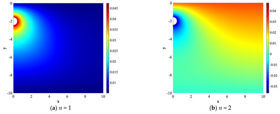
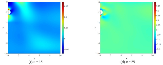
Figure 5.
Distributions of the typical POD basis functions applied to the steady situation.
Table 5.
Independency test of the selected basis function number.
Fifteen hidden neurons and twenty-five output neurons are used to construct the two-layered BP neural network, and the BP neural network is trained according to the spectrum coefficients and preset parameters of samples. The training process takes 345 s. The decay of the mean squared error with epochs and the regression plot of the testing set are shown in Figure 6. The mean squared error is from the sum of all grid cells and finally becomes approximately invariant. The correlation coefficient approaches one, thus the trained BP neural network can fit well with the mapping relationship between the input and output. Then, the preset parameters of five validation cases are inputted into the BP neural network to obtain the predicted spectrum coefficients. After that, substituting the predicted spectrum coefficients into the basis functions can reconstruct the predicted temperature field. Figure 7 presents the comparison of predicted temperature fields and accurate results. The POD-BP model successfully captures the temperature distribution trends of cases with different boundary conditions, thermal properties, and geometry parameters. It can be seen that the contours of the predicted temperature field are very consistent with the accurate results around the hot oil pipe, where the high-temperature gradient lies. The deviation of contours is larger on the region far from the pipe because the temperature changes are slight and hard to capture. There is no distinct regularity of error distribution among cases, as shown in the right subgraphs of Figure 7.
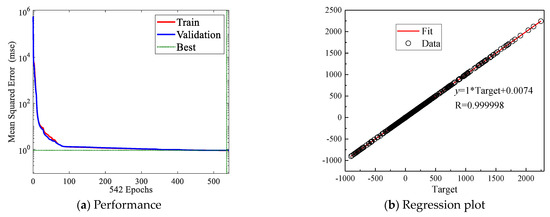
Figure 6.
For the BP neural network of the steady situation, (a) evolution of mean squared error with epochs and (b) regression plot of the testing set.
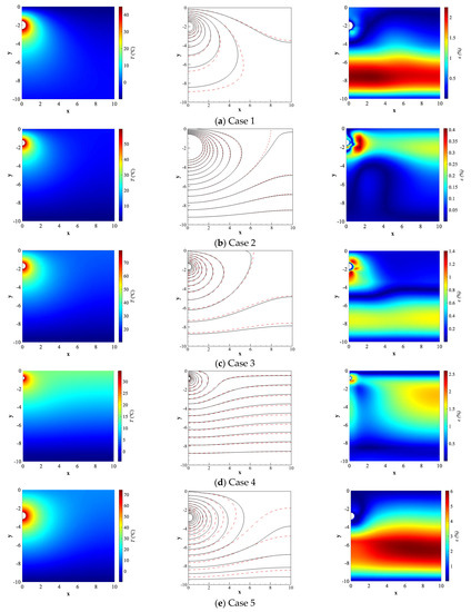
Figure 7.
Prediction results of the POD-BP model in the steady situation. The left subgraphs are accurate temperature distributions obtained by the FVM, the middle subgraphs are comparisons of contours of POD-BP prediction (dashed line) and FVM solutions (solid line), and the right subgraphs are error distributions.
The mean error and maximum error are shown in Table 6. Cases 1–4 have an error smaller than 2.599%, 2.247%, 0.406%, and 1.403%, respectively, but there is a relatively larger error for Case 5, which can reach 6.035%. This is because of the fact that Case 5 has both the boundary parameters (or property parameters) and geometry parameters outside the sampling range, making the temperature distribution significantly different from the samples.
Table 6.
Mean and maximum errors of multiple cases in the steady situation.
On the whole, the POD-BP model has high accuracy in predicting the steady temperature field surrounding the hot oil pipe and, in particular, it can successfully capture the variation caused by geometry parameters.
3.2. Unsteady Situation
For the unsteady situation, the initial temperature field is required for the simulation, and it is assumed that there is a linear distribution between Ta and Tc from the ground surface to the thermostatic layer. The calculation period is ten days and the discretized time step of the FVM is half an hour. However, the recorded time step used to establish the sample matrix is six hours, which ensures the computed size of the sample matrix is correct. Hence, each sampling condition has 40 temperature fields related to different moments, and the size of the sampling matrix is 3846×.
According to the singular-value decomposition method, 25,920 basis functions are obtained for the unsteady situation. Table 7 presents the eigenvalues, energy contribution, and accumulative energy of the first eight basis functions. It is observed that the first six basis functions can account for 99.9% of the total energy. Similar to the steady situation, the first and third basis functions have continuous distributions and significant gradients around the pipe, while the fifteenth and twenty-fifth basis functions have heterogeneous distributions to capture the local information, as shown in Figure 8. The first thirty basis functions are employed in the POD-BP model to predict the unsteady temperature field.
Table 7.
Eigenvalues of the first eight POD basis functions in the unsteady situation.
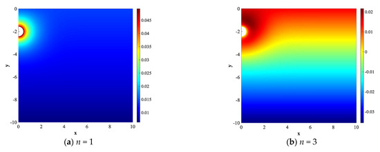
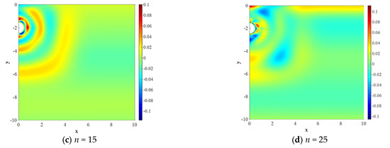
Figure 8.
Distributions of the typical POD basis functions applied to the unsteady situation.
The BP neural network consists of fifteen hidden neurons and thirty output neurons, and its training process takes 2778 s. Figure 9 shows the performance with epochs and the regression plot of the testing set for the trained BP neural network. After that, the preset parameters of five validation cases corresponding to the second and tenth days are inputted into the BP neural network to obtain the predicted spectrum coefficients. Figure 10 and Figure 11 present the comparison of predicted temperature fields and accurate results for the second and tenth days, respectively. It can be observed that our present model can effectively calculate the temperature evolution with time, in which the region having distinct temperature disturbance becomes larger. In general, the POD-BP model can obtain temperature fields and contours comparable to the accurate results in the unsteady situation.
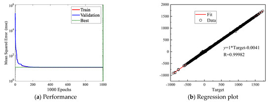
Figure 9.
For the BP neural network of the unsteady situation, (a) evolution of mean squared error with epochs and (b) regression plot of the testing set.
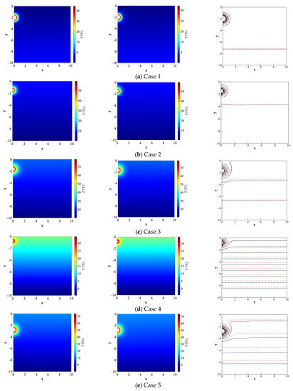
Figure 10.
Prediction results of the POD-BP model in the unsteady situation on the second day. The left subgraphs are accurate temperature distributions obtained by the FVM, the middle subgraphs are POD-BP results, and the right subgraphs are comparisons of POD-BP predicted contours (dashed line) and FVM solutions (solid line).
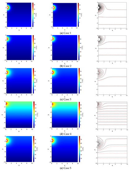
Figure 11.
Prediction results of POD-BP in the unsteady situation on the tenth day. The left subgraphs are accurate temperature distributions obtained by the FVM, the middle subgraphs are POD-BP results, and the right subgraphs are comparisons of POD-BP predicted contours (dashed line) and FVM solutions (solid line).
Table 8 presents the quantitative errors of five cases at the moments of the second day and tenth day, where the mean error of the PO-BP model is 0.133~1.439% and the maximum error falls at 0.885~7.058%. Appealingly, the 10-day simulation of FVM needs around 70 s to compute, while the POD-BP model consumes a very short time that can be ignored. This is because the neural network is applied directly in the POD-BP model, and no discretization equations of spectrum coefficients are solved.
Table 8.
Mean and maximum errors and computational time of multiple cases in the unsteady situation.
4. Conclusions
The fast prediction of the temperature field surrounding a hot oil pipe is important for the optimal design and risk assessment of the pipeline system. This paper proposes a novel POD-BP model to predict the temperature field surrounding a hot oil pipe efficiently. Unlike the classical POD reduced-order model, the BP neural network is adopted here to directly output the spectrum coefficients of the predicted sample according to its preset parameters. Moreover, introducing the BP neural network can omit the complex mathematical derivation of reduced-order governing equations and the solving of the spectrum coefficients system.
Then, we use the presented model to predict the temperature field surrounding the hot oil pipe in both steady and unsteady situations. The sample matrix is constructed based on the numerical results of FVM with 3846 grid cells. Three boundary parameters, one thermal property, and eight geometry structures are selected as the preset parameters of samples, which are comprehensive and rigorous for verification. Five validation cases with completely different preset parameters, including geometry parameters of buried depth and pipe diameter, are tested. The results show that our model can predict the temperature fields comparable to the FVM; the mean errors are 0.845~3.052% and 0.133~1.439% for steady and unsteady situations, respectively; and the max errors are 0.406~6.035% and 0.885~7.058%, respectively. What is more important is that there is almost no computation time for unsteady prediction using our model.
Our future work will concentrate on improving the prediction accuracy of the POD-BP model. First, an advanced network framework, such as the Bayesian neural network, can replace the two-layered BP network to robustly capture the mapping relationship. Second, the preset parameters of samples and recorded time steps in the unsteady situation will be optimized to obtain a series of basis functions with more accuracy.
Author Contributions
Conceptualization, F.Y. and D.H.; Formal analysis, K.J.; Methodology, F.Y., K.J. and D.H.; Project administration, C.N. and Q.L.; Software, K.J.; Validation, C.N. and Y.C.; Visualization, F.Y. and D.H.; Writing—original draft, K.J.; Writing—review and editing, F.Y. All authors have read and agreed to the published version of the manuscript.
Funding
This study is supported by the PipeChina unveiled project titled “Research on Safe and efficient Transportation Guarantee Technology of Crude Oil pipelines”, SSCC202204.
Data Availability Statement
The data presented in this study are available on request from the corresponding author.
Conflicts of Interest
The authors declare no conflict of interest.
Nomenclature
| Roman Symbols | |
| am | Spectrum coefficient |
| A | Matrix of spectrum coefficients |
| cp | Specific heat capacity, J·kg−1·°C−1 |
| d | Inner diameter of the steel pipe, m |
| ha | Heat transfer coefficient between the soil and air, W·m−2·°C−1 |
| hoil | Heat transfer coefficient between the oil and the wax layer, W·m−2·°C−1 |
| H0 | Buried depth, m |
| K | Number of recorded moments |
| L | Number of sampling conditions |
| M | Number of selected basis functions |
| N | Number of grid cells |
| Q | Single sample matrix |
| S | Entire sample matrix |
| t | Time, s |
| T | Temperature, °C |
| Ta | Atmosphere temperature, °C |
| Tc | Temperature of the thermostatic layer, °C |
| Toil | Hot oil temperature, °C |
| x, y | Cartesian coordinate, m |
| Greek Symbols | |
| Thickness of the wax layer, m | |
| εi | Error of the ith grid cell |
| φ | Single basis function |
| Φ | Matrix of basis functions |
| λ | Thermal conductivity, W·m−1·°C−1 |
| λn | Eigenvalue of the nth basis function |
| ζn | Energy contribution of the nth basis function |
| Accumulative energy of the first n basis functions | |
| ρ | Density, kg·m−3 |
| τ | Simulation time step |
| Subscripts | |
| 1, 2, 3, s | Layers of wax, steel, corrosion protection, and soil |
References
- Energy Institute. Statistical Review of World Energy. 2023. Available online: https://www.energyinst.org/statistical-review (accessed on 21 July 2023).
- Dey, P.K. Oil Pipelines. In Encyclopedia of Energy; Cleveland, C., Ed.; Elsevier: New York, NY, USA, 2004; pp. 673–690. ISBN 978-0-12-176480-7. [Google Scholar] [CrossRef]
- Yu, B.; Li, C.; Zhang, Z.; Liu, X.; Zhang, J.; Wei, J.; Sun, S.; Huang, J. Numerical simulation of a buried hot crude oil pipeline under normal operation. Appl. Therm. Eng. 2010, 30, 2670–2679. [Google Scholar] [CrossRef]
- Martínez-Palou, R.; Mosqueira de Lourdes, M.; Zapata-Rendón, B.; Mar-Juárez, E.; Bernal-Huicochea, C.; de la Cruz Clavel-López, J.; Aburto, J. Transportation of Heavy and Extra-Heavy Crude Oil by Pipeline: A Review. J. Pet. Sci. Eng. 2011, 75, 274–282. [Google Scholar] [CrossRef]
- Wang, K.; Zhang, J.J.; Yu, B.; Zhou, J.; Qian, J.H.; Qiu, D.P. Numerical Simulation on the Thermal and Hydraulic Behaviors of Batch Pipelining Crude Oils with Different Inlet Temperatures. Oil Gas Sci. Technol.—Rev. IFP 2009, 64, 503–520. [Google Scholar] [CrossRef]
- Wang, Y.; Wei, N.; Wan, D.; Wang, S.; Yuan, Z. Numerical Simulation for Preheating New Submarine Hot Oil Pipelines. Energies 2019, 12, 3518. [Google Scholar] [CrossRef]
- Dong, H.; Zhao, J.; Zhao, W.; Si, M.; Liu, J. Study on the Thermal Characteristics of Crude Oil Pipeline during Its Consecutive Process from Shutdown to Restart. Case Stud. Therm. Eng. 2019, 14, 100434. [Google Scholar] [CrossRef]
- Wei, L.; Lei, Q.; Zhao, J.; Dong, H.; Yang, L. Numerical Simulation for the Heat Transfer Behavior of Oil Pipeline during the Shutdown and Restart Process. Case Stud. Therm. Eng. 2018, 12, 470–483. [Google Scholar] [CrossRef]
- Jiao, K.; Wang, P.; Wang, Y.; Yu, B.; Bai, B.; Shao, Q.; Wang, X. Study on the multi-objective optimization of reliability and operating cost for natural gas pipeline network. Oil Gas Sci. Technol. 2021, 76, 42. [Google Scholar] [CrossRef]
- Białecki, R.; Kassab, A.; Fic, A. Proper orthogonal decomposition and modal analysis for acceleration of transient FEM thermal analysis. Int. J. Numer. Methods Eng. 2005, 62, 774–797. [Google Scholar] [CrossRef]
- Wang, L.; Dong, X.; Jing, L.; Li, T.; Zhao, H.; Zhang, B. Research on digital twin modeling method of transformer temperature field based on POD. Energy Rep. 2023, 9, 299–307. [Google Scholar] [CrossRef]
- Dong, Z.; Pan, C.; Wang, J.; Yuan, X. Reduced-order representation of superstructures in a turbulent boundary layer. Phys. Fluids 2023, 35, 55146. [Google Scholar] [CrossRef]
- Yang, T.; Zhao, P.; Zhao, Y.; Yu, T. Development of reduced-order thermal stratification model for upper plenum of a lead–bismuth fast reactor based on CFD. Nucl. Eng. Technol. 2023, 55, 2835–2843. [Google Scholar] [CrossRef]
- Ge, M.; Zhang, G.; Petkovšek, M.; Long, K.; Coutier-Delgosha, O. Intensity and regimes changing of hydrodynamic cavitation considering temperature effects. J. Clean. Prod. 2022, 338, 130470. [Google Scholar] [CrossRef]
- Hijazi, S.; Stabile, G.; Mola, A.; Rozza, G. Data-driven POD-Galerkin reduced order model for turbulent flows. J. Comput. Phys. 2020, 416, 109513. [Google Scholar] [CrossRef]
- Orellano, A.; Wengle, H. POD Analysis of Coherent Structures in Forced Turbulent Flow over a Fence. J. Turbul. 2001, 2, 008. [Google Scholar] [CrossRef]
- Antoranz, A.; Ianiro, A.; Flores, O.; García-Villalba, M. Extended proper orthogonal decomposition of non-homogeneous thermal fields in a turbulent pipe flow. Int. J. Heat Mass Transf. 2018, 118, 1264–1275. [Google Scholar] [CrossRef]
- Yu, G.; Yu, B.; Han, D.; Wang, L. Unsteady-state thermal calculation of buried oil pipeline using a proper orthogonal decomposition reduced-order model. Appl. Therm. Eng. 2013, 51, 177–189. [Google Scholar] [CrossRef]
- Yu, B.; Yu, G.; Cao, Z.; Han, D.; Shao, Q. Fast calculation of the soil temperature field around a buried oil pipeline using a body-fitted coordinates-based POD-Galerkin reduced-order model. Numer. Heat Transf. Part A Appl. 2013, 63, 776–794. [Google Scholar] [CrossRef]
- Han, D.; Yu, B.; Chen, J.; Wang, Y.; Wang, Y. POD reduced-order model for steady natural convection based on a body-fitted coordinate. Int. Commun. Heat Mass Transf. 2015, 68, 104–113. [Google Scholar] [CrossRef]
- Yu, J.; Ray, D.; Hesthaven, J.S. Fourier Collocation and Reduced Basis Methods for Fast Modeling of Compressible Flows. Commun. Comput. Phys. 2022, 3, 595–637. [Google Scholar] [CrossRef]
- Du, G.; Liu, Z.; Lu, H. Application of innovative risk early warning mode under big data technology in Internet credit financial risk assessment. J. Comput. Appl. Math. 2021, 386, 113260. [Google Scholar] [CrossRef]
- Wang, S.; Zhang, N.; Wu, L.; Wang, Y. Wind speed forecasting based on the hybrid ensemble empirical mode decomposition and GA-BP neural network method. Renew. Energy 2016, 94, 629–636. [Google Scholar] [CrossRef]
- Druault, P.; Delville, J.; Bonnet, J.-P. Proper Orthogonal Decomposition of the mixing layer flow into coherent structures and turbulent Gaussian fluctuations. Comptes Rendus Mécanique 2005, 333, 824–829. [Google Scholar] [CrossRef]
- Blazek, J. (Ed.) Chapter 3—Principles of Solution of the Governing Equations. In Computational Fluid Dynamics: Principles and Applications, 3rd ed.; Butterworth-Heinemann: Oxford, UK, 2015; pp. 29–72. ISBN 978-0-08-099995-1. [Google Scholar] [CrossRef]
- Lumley, J.L. Coherent Structures in Turbulence. In Transition and Turbulence; Meyer, R.E., Ed.; Academic Press: Cambridge, MA, USA, 1981; pp. 215–242. ISBN 978-0-12-493240-1. [Google Scholar] [CrossRef]
- Qin, S.; Li, J.; Chen, J.; Bi, X.; Xiang, H. Research on Displacement Efficiency by Injecting CO2 in Shale Reservoirs Based on a Genetic Neural Network Model. Energies 2023, 16, 4812. [Google Scholar] [CrossRef]
- Irfan, M.M.; Malaji, S.; Patsa, C.; Rangarajan, S.S.; Hussain, S.M.S. Control of DSTATCOM Using ANN-BP Algorithm for the Grid Connected Wind Energy System. Energies 2022, 15, 6988. [Google Scholar] [CrossRef]
- Moré, J.J. The Levenberg-Marquardt algorithm: Implementation and theory. In Lecture Notes in Mathematics: Numerical Analysis; Watson, G.A., Ed.; Springer: Berlin/Heidelberg, Germany, 1978; pp. 105–116. ISBN 978-3-540-35972-2. [Google Scholar] [CrossRef]
- Christou, V.; Arjmand, A.; Dimopoulos, D.; Varvarousis, D.; Tsoulos, I.; Tzallas, A.T.; Gogos, C.; Tsipouras, M.G.; Glavas, E.; Ploumis, A.; et al. Automatic Hemiplegia Type Detection (Right or Left) Using the Levenberg-Marquardt Backpropagation Method. Information 2022, 13, 101. [Google Scholar] [CrossRef]
Disclaimer/Publisher’s Note: The statements, opinions and data contained in all publications are solely those of the individual author(s) and contributor(s) and not of MDPI and/or the editor(s). MDPI and/or the editor(s) disclaim responsibility for any injury to people or property resulting from any ideas, methods, instructions or products referred to in the content. |
© 2023 by the authors. Licensee MDPI, Basel, Switzerland. This article is an open access article distributed under the terms and conditions of the Creative Commons Attribution (CC BY) license (https://creativecommons.org/licenses/by/4.0/).