1. Introduction
Drilling plays a crucial role in the exploration and development of oil and gas fields. Drilling typically constitutes over 50% of the investment expenses for oil and gas well development. Non-productive time (NPT), required to manage complex situations and accidents during drilling, comprises approximately 6% to 8% of the total construction duration [
1]. Thus, enhancing drilling safety and efficiency holds paramount importance in improving oil and gas field development efficiency.
Various factors influence the safety and efficiency of drilling operations [
2], encompassing geological, engineering, and human aspects. Examples include geological conditions, wellbore stability, drilling fluid performance, equipment conditions, construction influence, personnel expertise, and on-site experience [
3]. These factors contribute to challenging scenarios during drilling, like wellbore collapse, leakage, and pipe blockage [
4,
5,
6]. Drilling accidents not only prolong operations and escalate costs, but they can also cause severe incidents, including blowouts, leading to well abandonment [
7].
Designing a secure drilling fluid density window is essential to prevent complex drilling scenarios. Typically, the formation pore pressure sets the lower limit for the secure drilling fluid density window. Thus, precise prediction of the formation pore pressure is highly important to ensure both safety and efficiency in drilling operations.
Subsequent to the 1990s, researchers revealed that diverse pressure mechanisms within geological formations necessitate the adoption of distinct pore pressure prediction models; otherwise, substantial errors may arise in the forecasting outcomes. A statistical analysis of formation pressures in more than 100 oil fields revealed that high-pressure oil and gas reservoirs constitute the predominant share, comprising 47.7%. This finding indicates that abnormally high pressure is a prevalent issue in oil and gas exploration and development. Consequently, precise identification of the formation mechanism causing abnormal high pressure and the appropriate selection of a suitable pore pressure prediction model are vital for significantly enhancing the accuracy of predictions. This holds paramount importance in guaranteeing safe and efficient drilling and construction during oil and gas exploration and development.
Bowers conducted comprehensive experimental research focusing on the Gulf of Mexico region to determine pressure mechanisms. During the study, Bowers [
8] observed distinct well logging data responses in formations with either undercompaction or fluid expansion. In undercompacted formations, the relationship between acoustic velocity and effective stress follows the loading mechanism, whereas in fluid-expanded formations, it follows the unloading mechanism. Furthermore, Bowers [
9] proposed that the intersection plot of the formation density and acoustic time difference (or acoustic velocity) can distinguish between the loading and unloading mechanisms. Stephen’s research [
10] revealed that in formations that are not entirely sealed, processes like mineral transformation and hydrocarbon generation can result in increased porosity of the rock skeleton, damage to rock pores, and alterations in the cementation of the skeleton. Subsequently, these processes cause an increase in formation density and a decrease in acoustic velocity.
Accurate pore pressure predictions necessitate not only identifying the pressure mechanisms causing abnormal high pressure, but also selecting an appropriate prediction model. Formation pore pressure prediction methods can be classified into three main types based on different criteria [
11]: pre-drilling prediction, real-time monitoring while drilling, and post-drilling detection. Pore pressure prediction methods can be further categorized based on data sources into two types: one utilizes well logging data feedback from oilfields for pressure prediction, known as the drilling data analysis method, while the other involves establishing empirical models between geophysical parameters and various rock mechanical parameters in geophysical exploration. Eaton [
12] proposed the rudimentary form of the Eaton formula based on the principle of effective stress, which was further improved and is still widely used for predicting abnormal high pressure caused by undercompacted mudrocks [
13]. Bowers [
8] categorized the formation of abnormal pressure into loading and unloading processes and provided pore pressure prediction methods for these mechanisms, which are still widely used today [
9]. Ziegler [
14] and colleagues calculated formation pore pressure using the Bowers formula and other methods, subsequently calibrating it with real-time drilling data. Liu [
15] proposed a novel formula for predicting pore pressure based on formation velocity data, considering the principles of effective stress and the granular pile model. Liu [
16] introduced a pore pressure prediction method tailored for carbonate formations and applied it in the Sichuan Basin, yielding relative prediction errors ranging from 0.60% to 10.22%. As conventional oil and gas exploration and development increasingly shift towards complex unconventional resources, the limitations of traditional formation pore pressure prediction methods, including limited applicability, susceptibility to human factors, and significant constraints, have become apparent.
Artificial Intelligence (AI) refers to the scientific field focused on developing intelligent tools, devices, systems, and other innovations. This field includes subfields like machine learning and deep learning [
17,
18]. Due to their substantial advantages in tackling complex nonlinear problems, machine learning algorithms have gained wide popularity among scholars. Machine learning algorithms intelligently identify patterns within sample data, facilitating the classification or prediction of unknown data. Compared to traditional empirical formula methods, this approach demonstrates greater accuracy, objectivity, and efficiency, finding extensive applications in various sectors of the petroleum industry [
19,
20,
21,
22,
23,
24,
25]. For example, Fares Abu-Abed [
4,
5,
6] introduced a pattern recognition approach utilizing artificial neural networks for the identification and prediction of intricate scenarios within the drilling process. The approach employs accident statistical data extracted from the database as its input and enables the prediction of accidents, including blowouts, well leaks, and wellbore collapses. A neural network model has been developed by Shahboz Qodirov and his team, employing a sliding window approach. The model is capable of offering real-time predictions regarding occurrences of stuck pipe incidents within the drilling process, achieving prediction accuracy levels reaching up to 86% [
7].
Notable progress has been made in recent years regarding the use of machine learning algorithms for pore pressure prediction. R. Keshavarzi [
26] highlighted the significant limitations of traditional pore pressure prediction methods based on empirical coefficients. To address this, he employed a BP neural network to predict the pore pressure gradient in the Asmari oilfield, Iran, and compared it with the Eaton method. Abdulmalek Ahmed [
27] proposed a high-precision pore pressure prediction method based on drilling parameters, including Weight on Bit (WOB), Rate of Penetration (ROP), and well logging data, employing an improved Artificial Neural Network (ANN). The average prediction error was 0.17%. Huang and colleagues [
28] established a pore pressure prediction model for sandy mudstone formations, employing five machine learning algorithms, including support vector machine and Random Forest. The model incorporated four input layer data: longitudinal velocity, porosity, mud content, and density. Overall, significant progress has been made in recent years in using machine learning methods to predict pore pressure; however, it is still primarily limited to predicting pore pressure in normal-pressure blocks. Nevertheless, there is limited research on predicting pore pressure in blocks with abnormal high pressure.
Conventional techniques for reservoir pore pressure prediction, exemplified by the Eaton and Bowers methods, necessitate an abundance of empirical parameters and intricate computations. Thus, a pressing requirement arises for novel approaches capable of efficiently, effortlessly, and precisely forecasting reservoir pore pressure. Presently, research related to the utilization of machine learning techniques for reservoir pore pressure prediction primarily centers on zones characterized by normal pressure. Addressing the research gap in using machine learning methods to predict pore pressure in blocks with abnormal high pressure, this paper focuses on the engineering case of well X-1 and employs two methods to analyze the abnormal high-pressure formation mechanism in this block. Subsequently, the Bowers method was employed for pore pressure prediction once the pressure mechanism was determined. The predicted values were compared with the measured pore pressure for error analysis and served as the learning sample data for the output layer of the model. Moreover, three well logging data, namely, delta t (DT), gamma logging (GR), and formation density logging (ZDEN), were chosen as the learning sample data for the input layer of the model. Four distinct machine learning algorithms were employed to establish intelligent pore pressure prediction models. The best-performing model was chosen for predicting the pore pressure in two adjacent wells near well X-1.
2. Theories and Methods
2.1. Method for Judging the Mechanism of Abnormal-Pressure Formation
Abnormal high pressure primarily results from fluids in the formation’s pores being subjected to the overlying rock pressure, which should have been borne by the surrounding rocks. Conversely, abnormal low pressure occurs when the surrounding rocks bear the overlying rock pressure that should have been sustained by the fluids around the pores. Presently, the mechanisms leading to abnormal pressure can be broadly categorized as follows [
29]:
- (1)
Changes in the volume of formation rock pores, such as lateral tectonic loading and imbalanced sedimentation (undercompaction).
- (2)
Changes in fluid volume within the pores, such as variations in temperature, hydrocarbon generation, and fluid migration.
- (3)
Fluid flow and pressure changes within the formation, such as pressure depletion resulting from oil and gas production.
While the formation of abnormal pressure involves various mechanisms and is often the result of the combined effects of multiple factors, the petroleum industry primarily focuses on hydrocarbon generation and sediment undercompaction as the main causes of abnormal high pressure.
The origins of formation overpressure are intricate and varied. However, they can be categorized into two mechanical perspectives: loading and unloading. The formation mechanisms of the loading curve include normal compaction and undercompaction. Normal compaction is a continuous loading process, whereas undercompaction involves gradual loading or a cessation of loading, resulting in a linear increase or unchanged vertical effective stress. Conversely, the formation mechanisms of the unloading curve are primarily attributed to hydrocarbon generation, fluid expansion, etc., leading to a reduction in vertical effective stress compared to the normal-pressure segment.
Throughout the process of sedimentary compaction and consolidation within geological strata, the mounting pressure from overlying rock layers causes gradual sediment compaction. Consequently, this results in elevated vertical effective stress and reduced porosity. The sediment undergoes a continuous mechanical loading process. Rock density augments with sedimentation depth, while sound wave velocity can serve as an indicator of the rock’s conductivity characteristics. As porosity diminishes throughout the loading process, sound wave velocity progressively rises. This phenomenon signifies a loading mechanism within geological strata.
During the process of sediment compaction or subsequent to it, certain factors, including hydrocarbon generation, can lead to an elevation in pore pressure or a reduction in overlying pressure. These changes result in a decrease in vertical effective stress and a concurrent increase in porosity, initiating a continuous mechanical unloading process within the sediment. This process is accompanied by a gradual attenuation in the variation of rock density with increasing depth. As porosity continues to increase throughout the unloading process, a notable and progressive reduction in sound wave velocity becomes evident. Consequently, this phenomenon distinctly signifies an unloading mechanism within geological strata.
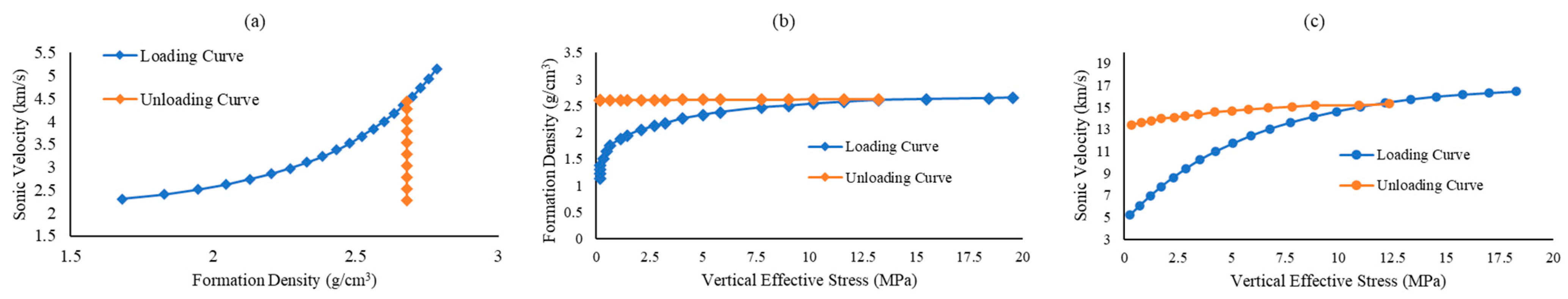
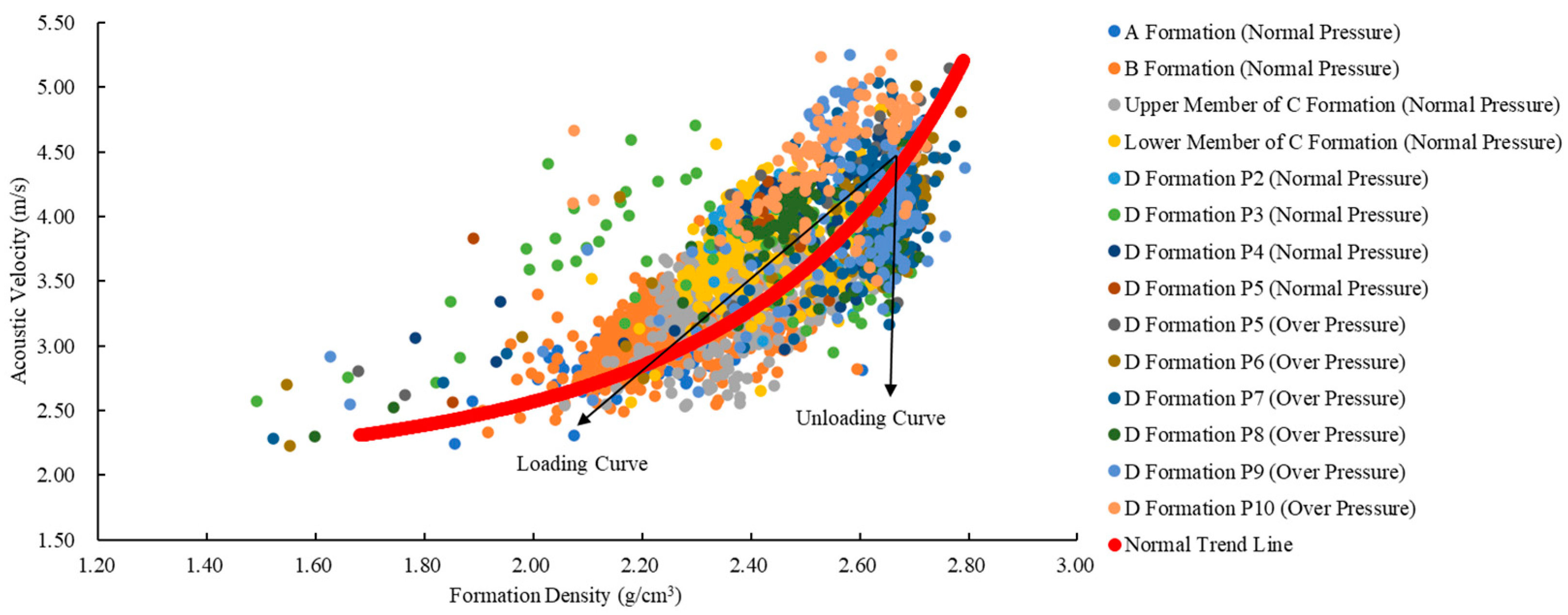
Bowers observed that during the unloading of formations, their longitudinal wave velocity decreases significantly, while their density exhibits a slight increase. The acoustic velocity reflects the rock’s conductivity, while the density represents its volumetric properties. The higher interconnected porosity in unloading formations compared to normal-pressure formations leads to a decrease in acoustic velocity. As shown in
Figure 1, with blue lines representing loading curves and orange lines representing unloading curves.
Figure 1a presents a formation density–acoustic velocity crossplot, illustrating an increase in formation density during the loading process, accompanied by a rise in longitudinal wave velocity. In contrast, the unloading curve forms nearly a vertical line, with density remaining almost constant and longitudinal wave velocity gradually decreasing. In
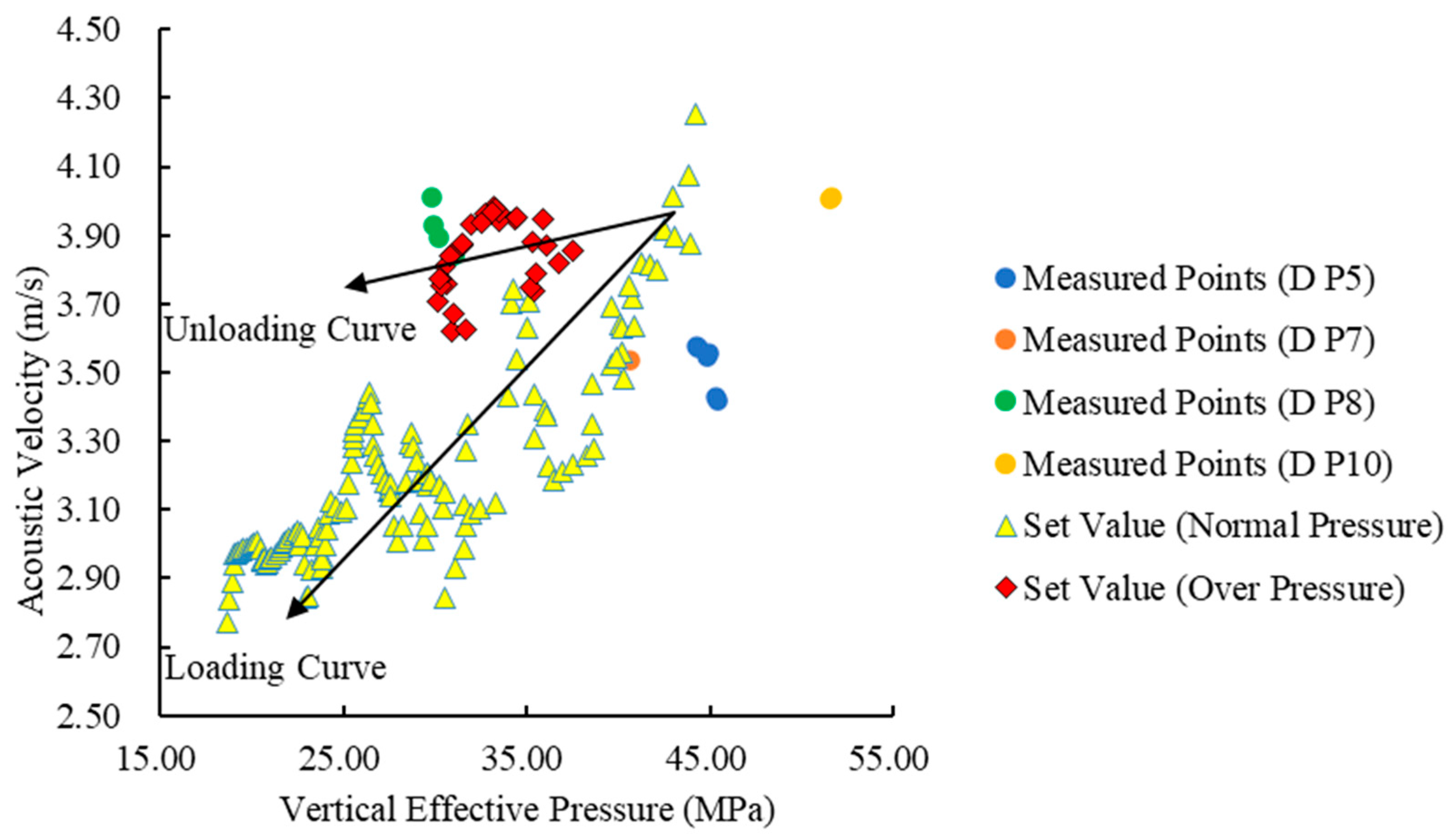
Figure 1b,c, the longitudinal wave velocity (or density) of loading formations increases significantly with the increase in vertical effective stress. Conversely, during the unloading process, the longitudinal wave velocity (or density) either changes slightly or remains constant with the decrease in vertical effective stress, indicating a gentle overall trend. The method of using
Figure 1b,c to ascertain the cause of abnormal pressure is referred to as the Bowers method. This paper combines the analyses of
Figure 1a–c to comprehensively determine the formation mechanism of abnormal pressure in the studied well and select the appropriate pore pressure prediction model based on this mechanism.
2.2. Pore Pressure Prediction Method
During sediment loading, the compaction effect of the overlying rock enhances the acoustic velocity of the formation. Conversely, during unloading, the acoustic velocity of the formation decreases. Considering the aforementioned phenomenon and based on the theory of effective stress, Bowers provided formulas describing the relationship between the acoustic velocity of the formation and effective stress under both loading and unloading conditions. The formula for the Bowers loading curve is as follows [
8,
30]:
The equation is defined as follows: V represents the longitudinal wave velocity in m/s, σ represents the vertical effective stress in MPa, and a and b are dimensionless parameters obtained by fitting existing data. The longitudinal wave velocity at the mudline, denoted as c, is commonly considered as 1524 m/s.
The formula for the Bowers unloading curve is as follows:
The equation introduces the unloading parameter
U, which is a dimensionless measure of rock’s plastic deformation, and
σmax, representing the maximum vertical effective stress at the onset of unloading. The value of
σmax is determined by Formula (3) and is expressed in MPa.
The equation includes Vmax, which represents the maximum acoustic velocity during unloading and is measured in m/s.
Additionally, if abnormal pressure is due to factors other than undercompaction, the vertical effective stress acting on the formation will be lower than the maximum vertical effective stress it has experienced in the past. Bowers establishes the connection between the loading curve and unloading curve using the formula below.
The equation includes σunl, representing the vertical effective stress used in the unloading curve in MPa; σl, representing the vertical effective stress used in the loading curve in MPa; and σin, representing the effective stress at the intersection point of the loading and unloading curves in MPa.
Based on this, Bowers also proposed a method to calculate pore pressure using acoustic time difference and maximum effective stress. The method is as follows:
If the depth
Hmax at which
Vmax occurs is greater than the total vertical depth
H, the formation has not undergone unloading, and the pore pressure is calculated using the following equation:
The equation includes Pp, representing the pore pressure in MPa; G, representing the overburden pressure in MPa; Δt, representing the acoustic time difference in seconds per meter (s/m); and Δtmax, denoting the acoustic time difference corresponding to Vmax in s/m.
If
Hmax ≤
H, which indicates that the formation has undergone unloading, the pore pressure (
Pp) is calculated using the following equation:
2.3. Machine Learning Algorithms
2.3.1. KNN
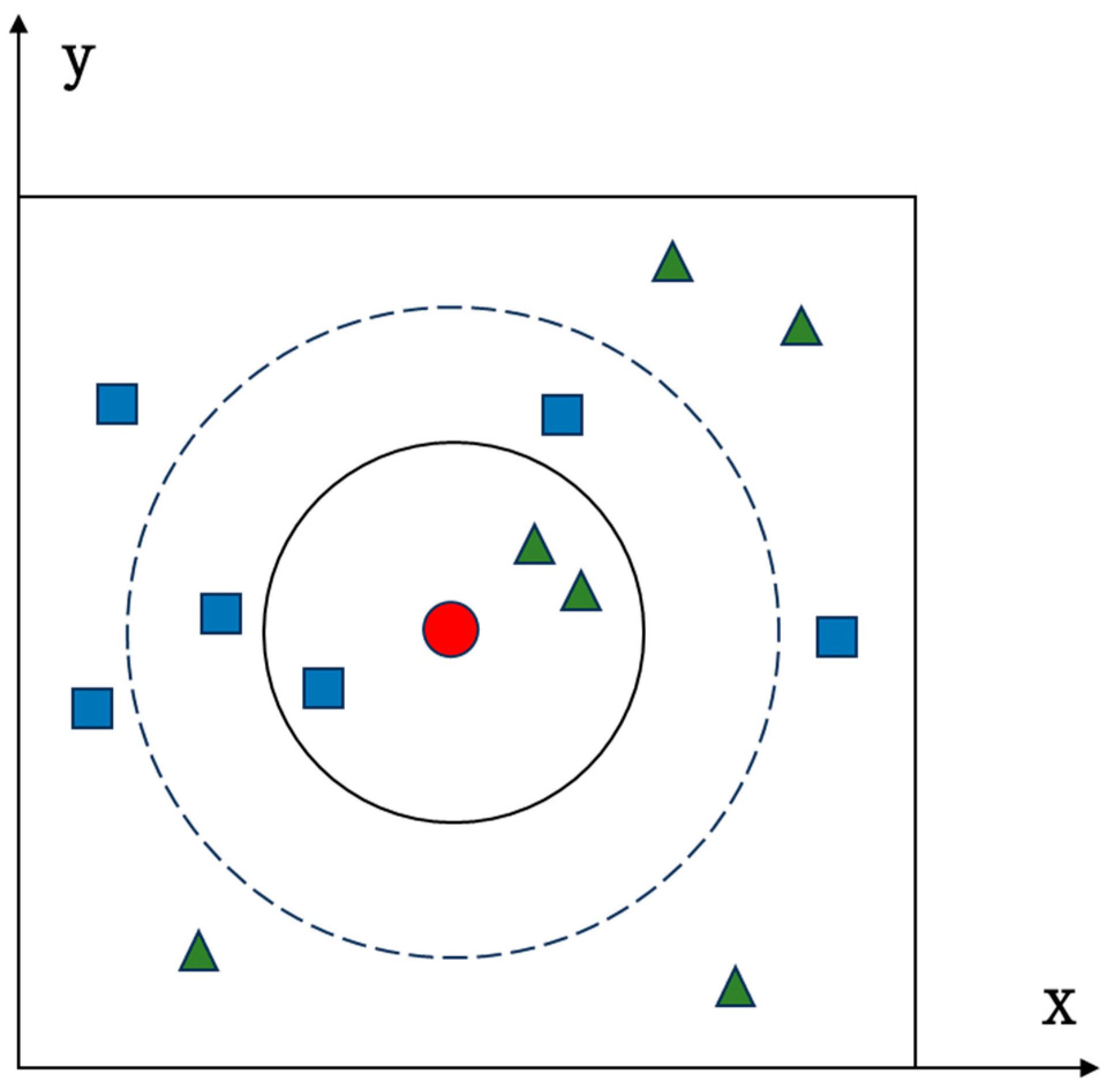
The K-Nearest Neighbor (KNN) algorithm exemplifies a “lazy learning” approach, known for its effectiveness in non-parametric regression and classification tasks based on historical data statistics. The structure of the KNN algorithm is depicted in
Figure 2. The algorithm’s dataset is partitioned into a training sample set and a testing sample set, with each data point in the dataset containing a label indicating its classification. The testing set maintains the same structure as the training sample set. To determine the classification of the test samples, the algorithm calculates the distances between the test samples and all samples in the training sample set. Subsequently, it selects the k nearest training samples based on the calculated distances. The final step involves determining the class of the test sample by counting the frequency of each class label among the k selected samples, where the most frequent label becomes the predicted class for the test sample [
31]. The steps of the KNN algorithm are as follows [
32]:
(1) Create the training sample set, denoted as X.
(2) Choose an initial value, k, for the number of nearest neighbors. Typically, the initial value is determined based on the specific circumstances and is continuously adjusted in subsequent experiments to identify the optimal value. No universally accepted standard exists for the initial selection and selection rules of k.
(3) Calculate the distance between the test sample,
y, and each sample in the training sample set individually, then select the nearest
k samples. Several methods exist to compute the proximity relationship between the test sample,
y, and each sample,
xi, in the training sample set, with the Euclidean distance being a common choice for measurement. Assuming sample
, the Euclidean distance between
y and
xi is defined as follows:
(4) For a given sample
xq with an undetermined category, let
x1,
x2, …,
xk represent the k nearest samples to y based on distance. Assuming the target function is discrete and denoted as
f:
Rn →
vi, where v
i represents the label of the
ith category, and the corresponding label set is
V = {
v1,
v2, …,
vs}, then the relationship can be expressed as follows:
The equation defines several key components: X signifies the training set; Y denotes the test set; xi and yi refer to the training and test samples, respectively; n represents the sample size; V corresponds to the label set; vi pertains to the label category; and xq symbolizes the sample awaiting classification.
2.3.2. Extra Trees
Extra Trees, short for Extremely Randomized Trees, represents a potent and versatile ensemble learning method derived from the traditional Decision Trees algorithm for machine learning tasks, including classification and regression. The structure of the Extra Trees algorithm is depicted in
Figure 3. It was proposed by Pierre Geurts, Damien Ernst, and Louis Wehenkel in 2006, aiming to introduce additional randomness during the tree construction process to minimize variance and enhance the model’s predictive accuracy. The distinctive “extremely random” feature of Extra Trees primarily lies in employing random features and random thresholds to split nodes in the decision tree. This approach introduces extra randomness, thereby increasing diversity and randomness across all decision trees. As a result, it effectively combats overfitting, while expediting the training process. Consequently, the algorithm demonstrates improved generalization and noise resistance, although at the expense of increased bias [
33].
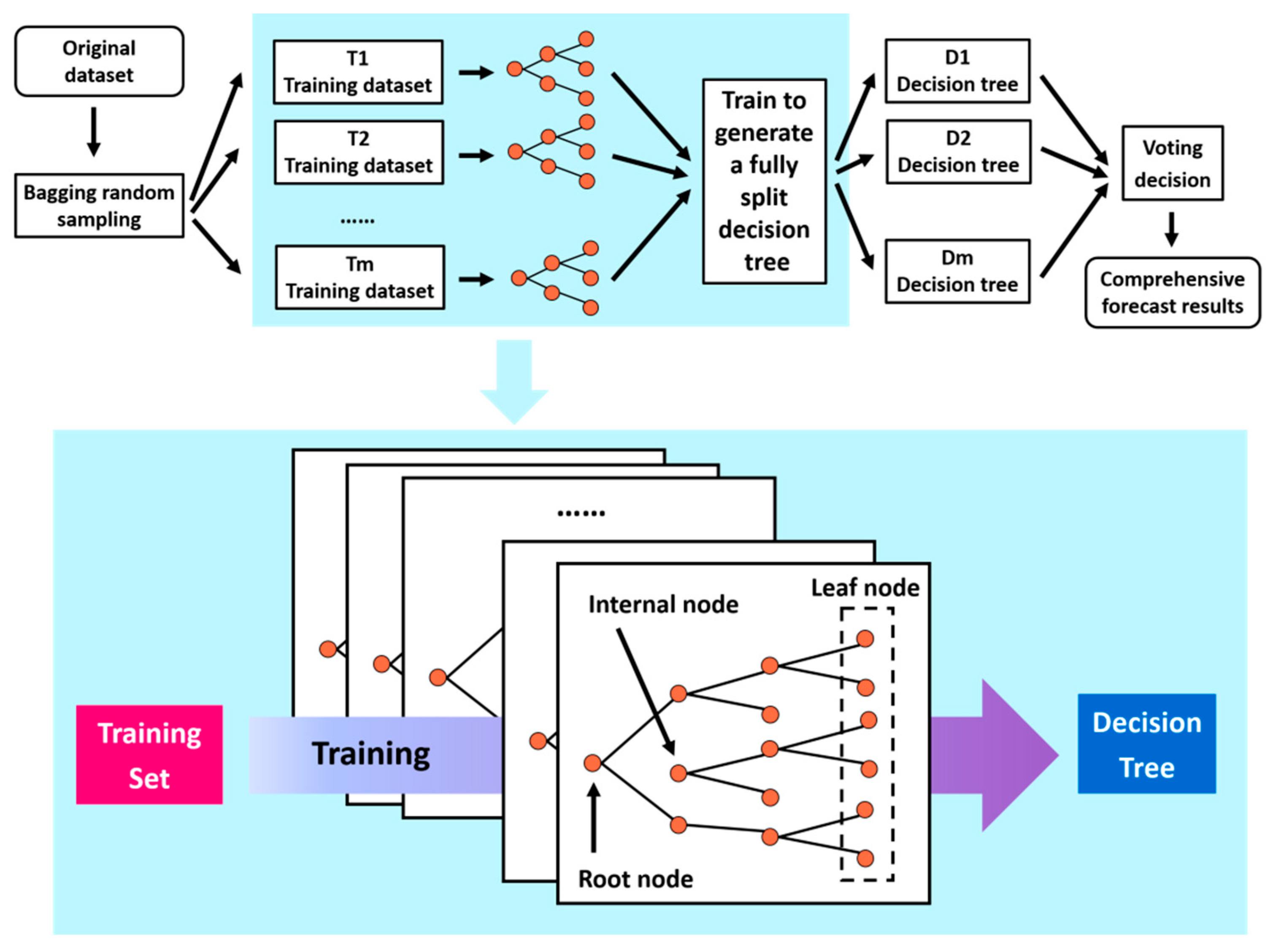
2.3.3. Random Forest
Random Forest (RF) represents a supervised machine learning method constructed by ensembling decision trees as base learners. It employs the bootstrap method to randomly sample multiple subsets, with replacement, from the original dataset. Each subset is then used to train a weak classifier, specifically, a decision tree. Subsequently, these decision trees are combined, and the final classification or prediction result is determined through majority voting [
34]. The introduction of randomness during the training process empowers Random Forest to exhibit excellent resistance to overfitting and noise [
35]. The structure of the Random Forest algorithm is depicted in
Figure 4. The training process of the Random Forest regression algorithm comprises four steps:
- (1)
Random and with-replacement sampling to train decision trees.
To create decision trees, the Bootstraping method is utilized for random and with-replacement sampling N times, with each sample containing one item, resulting in N subsets. Each subset serves as the sample at the root node of the tree and is used to train a decision tree. Importantly, different training sets are independent of each other.
- (2)
Randomly selecting attributes for node splitting.
At each node of the decision tree requiring splitting, m attributes are randomly chosen from the M attributes available in each sample, where m << M. Subsequently, from these m attributes, a specific strategy (e.g., information gain) is employed to determine the splitting attribute for that node.
- (3)
Repeating step (2) until no further splitting is possible.
Throughout the formation of the decision tree, each node is split according to step 2 repeatedly until no further splitting is feasible. The termination criterion for splitting is if the next attribute selected for the node is the same as the one used by its parent node during the last split. In this case, the node has reached a leaf node and requires no further splitting. Notably, no pruning occurs during the entire formation process of the decision tree.
- (4)
Establishing a large number of decision trees to form a forest.
The process is reiterated to build a substantial number of decision trees, collectively constituting the Random Forest. The final output result is determined by computing the average value of the outputs of all decision trees.
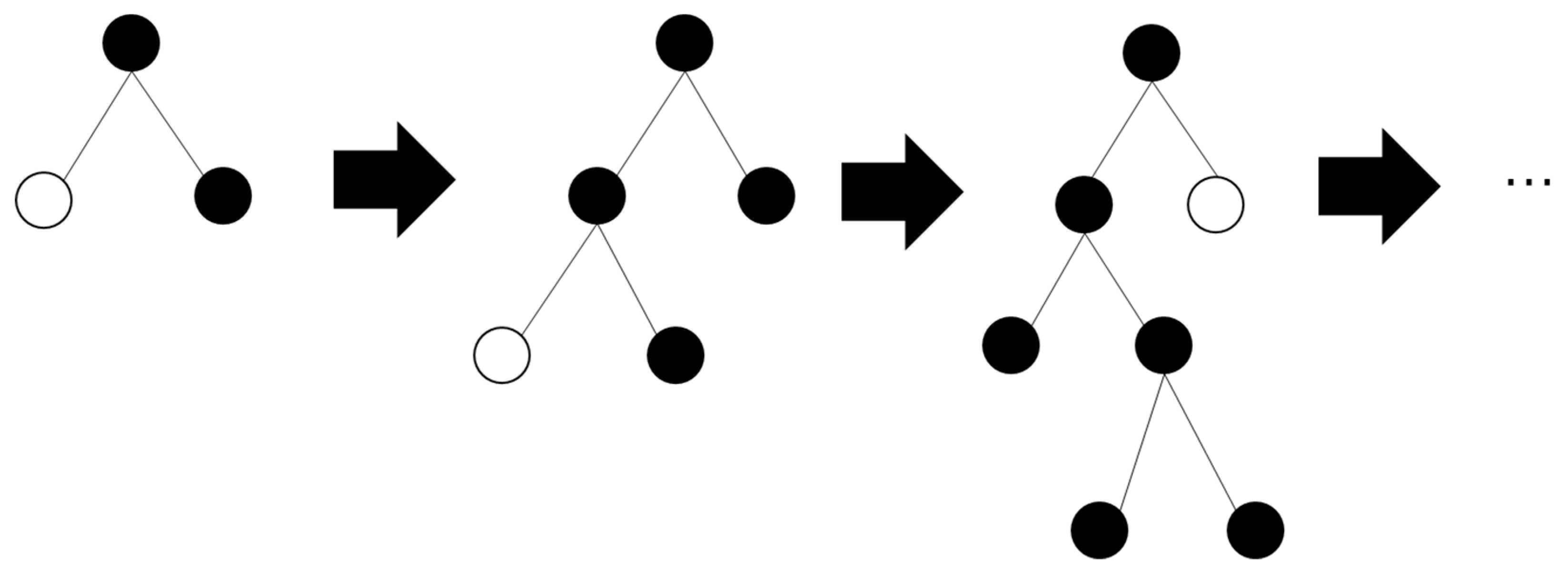
2.3.4. LightGBM
LightGBM (Light Gradient Boosting Machine) is an ensemble learning model based on the decision tree algorithm. It represents an efficient implementation of the GBDT (Gradient Boosting Decision Tree) model. In comparison to traditional GBDT models, LightGBM adopts the GOSS (Gradient-based One-side Sampling) algorithm to reduce the number of features and the EFB (Exclusive Feature Bundling) algorithm to enhance the histogram algorithm for feature processing. Its design philosophy revolves around two key aspects: first, optimizing memory utilization efficiency to leverage maximum data without compromising individual machine speed; and second, minimizing communication costs and enhancing parallel computing efficiency across multiple machines, resulting in linear computation [
36,
37]. The structure of the LightGBM algorithm is depicted in
Figure 5. The main advantages of the LightGBM algorithm include:
- (1)
During the process of finding split points, LightGBM significantly reduces the computational workload by introducing its histogram algorithm. This results in higher computational efficiency, while reducing memory usage during computation.
- (2)
LightGBM generates trees using leaf-wise splitting instead of level-wise splitting, enabling it to obtain more complex models, higher fitting capacity, and lower errors.
- (3)
LightGBM introduces three techniques: gradient-based one-side sampling, exclusive feature bundling, and histogram algorithms. These advancements enable it to handle massive data more effectively compared to other algorithms.
- (4)
The LightGBM algorithm supports parallel learning, further reducing the model’s computation time.
- (5)
LightGBM incorporates rules for classifying categorical features into the decision-making process, eliminating the need to convert them into numerical variables beforehand and allowing direct input of categorical feature data.
3. Results and Analysis
3.1. Geological Setting
The X Block in the BH Oilfield represents a typical area with abnormally high pressure, where the highest pore pressure coefficient can reach 1.6. Currently, there are three development wells in the X Block, namely, the X-1, X-2, and X-3 wells. Among them, X-1 is a vertical well, primarily targeting sandstone and gray shale, with some coal seams ranging from 1 to 2 m (
Figure 6). The geological conditions in this block are complex, giving rise to various mechanisms causing abnormal pressures. Pressures exceeding the norm are widespread in formations deeper than 3300 m. According to drilling results, the pore pressure coefficients of the main target formations generally range from 1.2 to 1.5, with some areas approaching 1.6. This phenomenon is closely related to the formation temperature and the maturity depth of source rocks. Additionally, the region’s sedimentary and tectonic history is intricate, experiencing multiple tectonic movements, resulting in non-uniform pressure systems among different blocks and narrow pressure windows. Overall, the vertical pressure characteristics in this area indicate that the shallow formations (up to approximately 3500 m, belonging to Formation C) maintain normal pressures, with the pore pressure equivalent density generally remaining around 1.0 g/cm
3, fluctuating within the range of −0.02 to +0.1 g/cm
3. However, in the mid-to-deep formations (approximately below 3500 m, from the lower section of Formation C to Formation D), the pore pressure increases significantly.
The main target formation of well X-1 is the lower section of Formation D, which serves as the primary hydrocarbon source rock layer in this block. It primarily comprises gray shale and siltstone shale, constituting nearly 60% of the total sediment thickness. Based on geochemical analysis results, the source rocks of Formation D began entering the mature stage at approximately 3500 m, with a peak hydrocarbon generation stage occurring at around 3800 m. The substantial oil and gas generated during the hydrocarbon generation process infiltrated the formation’s pores, leading to a significant increase in pore pressure. Remarkably, this observation aligns with the longitudinal distribution of pore pressure observed in other wells previously drilled in the X Block. Consequently, from a geological background perspective, the pressure increase induced by hydrocarbon generation has notably impacted the occurrence of deep, abnormal high pressure in the X Block.
3.2. Method for Identifying Overpressure Causes
This study integrates Bowers’ method and the acoustic velocity–density crossplot method to analyze the abnormal pressure in well X-1, building upon the previously described method for determining the abnormal high-pressure formation mechanism. The analysis involves plotting the effective stress–density crossplot, effective stress–acoustic velocity crossplot, and density–acoustic velocity crossplot for well X-1. A comprehensive comparative analysis of these three plots is then conducted. The overall approach is as follows:
- (1)
Select Mudstone Section Well Log Data and Divide Intervals.
The original well log data are organized and filtered to extract data from the mudstone sections. Subsequently, based on geological information obtained during drilling completion, the well log data for each well are divided into different intervals. For intervals requiring special attention, a more detailed division is performed. For instance, the C formation is further divided into upper and lower sections, while the primary target reservoir, D formation, is divided into three sections: upper, middle, and lower. The upper section encompasses layers P2 to P4, the middle section includes layers P5 to P7, and the lower section consists of layers P8 to P10 (refer to
Table 1).
- (2)
Drawing Well Depth–Density and Well Depth–LN(DT) Plots for Pressure Analysis.
To analyze the pressure conditions in well X-1, we utilize the well log data, primarily consisting of formation density and acoustic travel time (DT). Consequently, we plot the well depth–density and well depth–LN(DT) graphs, encompassing the entire well section. By examining the longitudinal distribution of pore pressure around the well, we ascertain the boundary between the normal-pressure and high-pressure intervals in well X-1. This division leads to the identification of two major sections within the well: the normal-pressure section and the high-pressure section. Typically, the high-pressure section is located in the middle-to-lower part of the D formation.
- (3)
Creating Crossplots and Trend Analysis for Pressure Evaluation in Well X-1.
We initiate the analysis by creating three crossplots: formation density vs. acoustic velocity, vertical effective stress vs. acoustic velocity, and vertical effective stress vs. formation density for well X-1. Initially, a scatter diagram of formation density vs. acoustic velocity is plotted for well X-1. Subsequently, we generate the well depth–formation density plot and well depth–LN(DT) plot to determine the normal trends of formation density and acoustic travel time within the well’s normal-pressure interval. Based on these trends, we construct the normal trend diagram. Next, acoustic travel time and formation density data are retrieved for the upper 3 m and lower 3 m of the measured pore pressure points. Their average values are calculated to determine the acoustic velocity. The well depth–formation density function is then fitted with this information. By utilizing this function, we compute the overburden pressure (
PS) and effective stress (
PY) corresponding to the measured pore pressure points using Formula (8). The obtained data are used to generate the crossplots of effective stress vs. acoustic velocity and effective stress vs. formation density. Since the availability of measured data points is often limited, the curves representing loading and unloading paths may not be clearly visible on the plots. To address this, it is common to set normal-pressure data points and high-pressure data points based on measured data from the target well or nearby wells, thereby obtaining distinct loading and unloading curves.
In the equation, PY denotes vertical effective stress (in MPa), PS stands for overburden pressure (in MPa), and PP represents pore pressure (in MPa).
Due to the influence of external factors and logging equipment, even in pure shale points, logging data, such as formation density, gamma, and sonic travel time, still have certain inaccuracies. Therefore, their loading and unloading curves cannot perfectly overlap with the ideal state of the plot. However, their data points still exhibit distinct distribution characteristics. From
Figure 7, it can be observed that as the well depth reaches the middle section of the D Formation, the formation density increases due to fluid expansion, while the sonic velocity decreases. Specifically, the data points from the lower part of the formation (below the P5 sand unit of the D Formation) deviate significantly from the normal trend line, exhibiting a clear unloading curve, which is consistent with the unloading mechanism caused by hydrocarbon generation pressure. X-1 well has a total of 13 measured pore pressure data points, all of which are located in the D Formation, with 4 high-pressure points (pore pressure coefficient greater than 1.2).
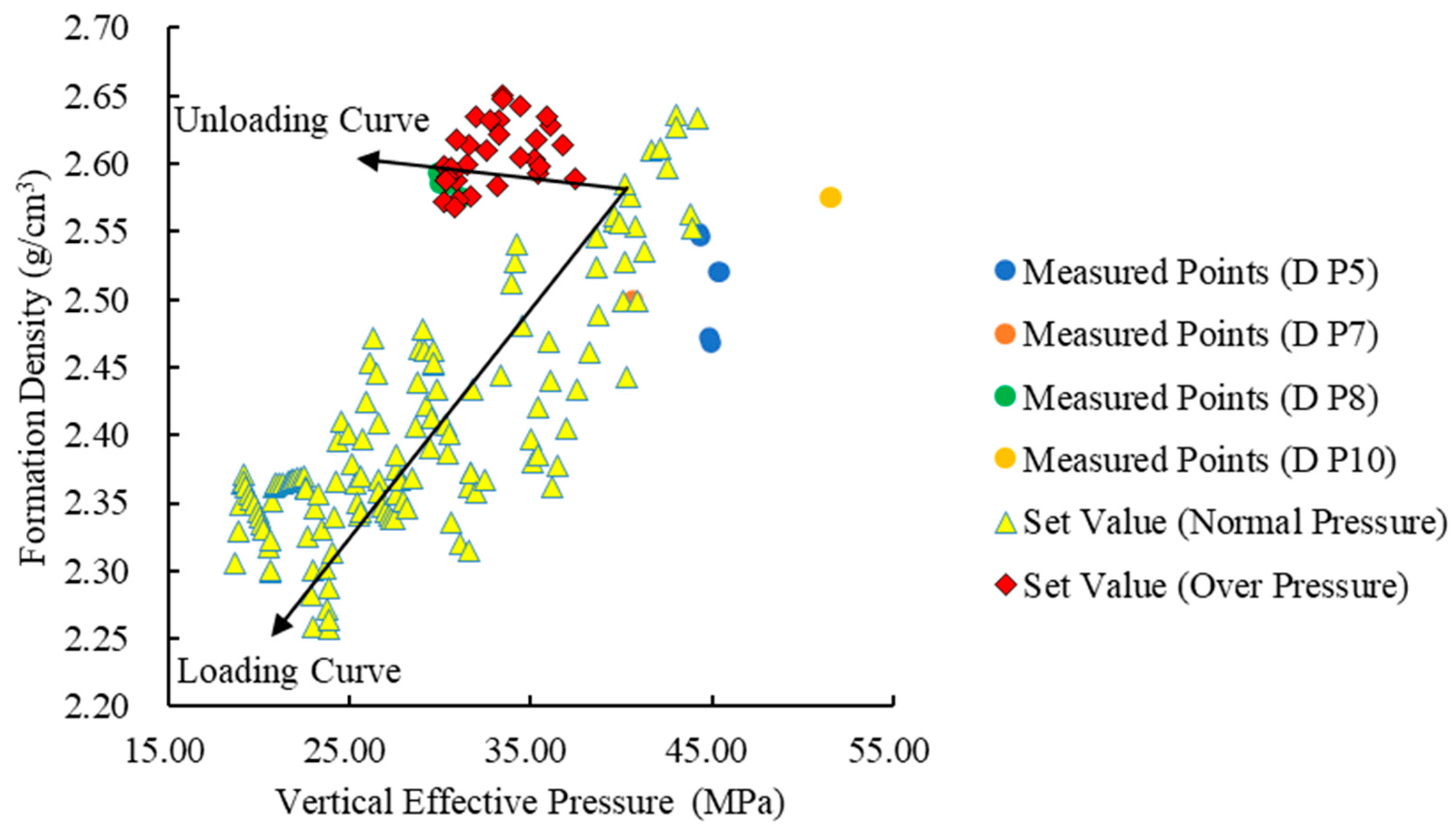
Figure 8 shows a very obvious linear increase trend between the set vertical effective stress and the longitudinal sonic velocity for the designated normal-pressure points. However, for both the measured high-pressure data points and the designated high-pressure data points, the vertical effective stress decreases significantly. This indicates that the depth has reached the hydrocarbon generation threshold, and the source rocks in the middle and lower sections of the D Formation have generated a large amount of oil and gas. The fluid expansion resulting from hydrocarbon generation pressure bears the part of the overlying rock pressure that should have been carried by the rock, leading to a rapid increase in pore pressure and displaying a clear unloading curve, once again confirming the unloading mechanism caused by hydrocarbon generation pressure.
Finally, from
Figure 9, it can be observed that the designated normal-pressure data points still exhibit a clear linear increase trend. As for the high-pressure data points, the vertical effective stress decreases significantly, while the formation density shows a slight increase compared to the designated normal-pressure data points. This still aligns with the geological understanding that high pressure is caused by hydrocarbon generation fluid expansion. In summary, the combination of the Bowers method and the sonic velocity–density crossplot analysis can effectively and accurately determine the formation mechanism of abnormal high pressure in the X-1 well. Specifically, the abnormal high pressure in the X-1 well is caused by hydrocarbon generation pressure.
3.3. Pore Pressure Calculation
As mentioned earlier, the X-1 well belongs to the unloading type of abnormal-pressure mechanism. Therefore, this study uses the Bowers method to calculate the pore pressure of the X-1 well and presents the longitudinal pore pressure profile of the X-1 well (see
Figure 10). In this study, well intervals with a pore pressure equivalent density below 1.2 g/cm
3 are considered as normal-pressure intervals, and intervals with a density above 1.2 g/cm
3 are considered as high-pressure intervals. Due to the existence of pressure reversal phenomena in the deep formations, intervals with a pore pressure equivalent density below 1.2 g/cm
3 in the deep formations are considered as pressure reversal intervals. From
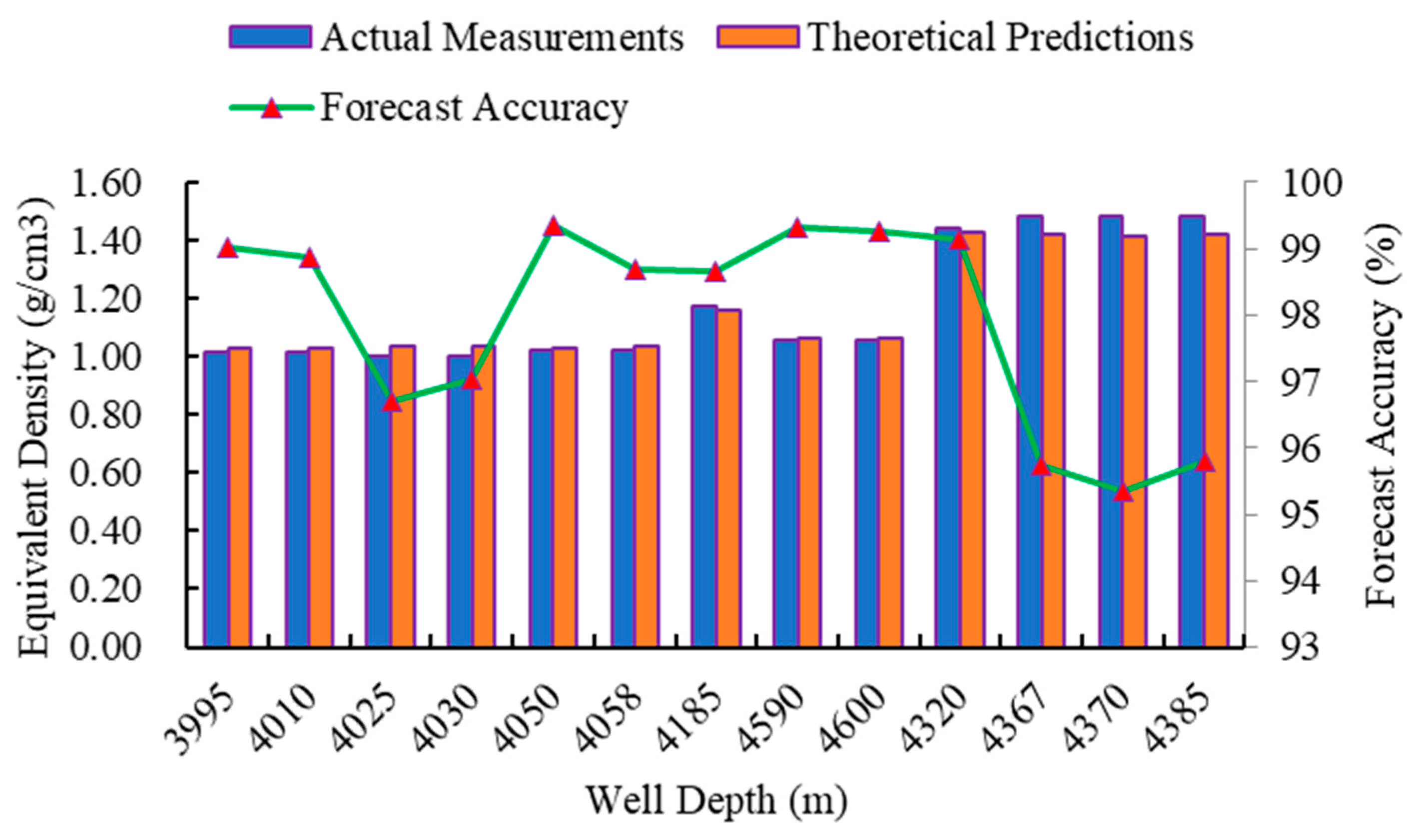
Figure 10, it can be observed that the normal-pressure interval of the X-1 well ranges from 2125 m to 4189 m. The high-pressure interval of the X-1 well starts at 4190 m (located in the middle section of the D Formation, P6 sand unit) and extends to 4519 m. The high-pressure interval is situated in the middle and lower sections of the D Formation, including the P6, P7, P8, P9, and P10 sand units. The increasing trend of pore pressure in the high-pressure interval exhibits clear step-like characteristics, with the maximum pore pressure equivalent density being 1.49 g/cm
3. However, from 4450 m (located in the lower section of the D Formation, P9 sand unit) onwards, the pore pressure drops significantly, showing pressure reversal characteristics. The depth range of the pressure reversal interval is from 4520 m to 4647 m. Based on the results from
Figure 11, the pore pressure calculated using the Bowers method has a prediction accuracy exceeding 95%, ranging from 95.350% to 99.360%. Therefore, according to the analysis of the abnormal-pressure mechanism and the calculation of the well logging data, the calculated pore pressure agrees well with the measured pore pressure, indicating that the calculated pore pressure can be considered as the true formation pore pressure.
3.4. Construction of Pore Pressure Prediction Model Based on Machine Learning Algorithms
3.4.1. Data Gathering and Preprocessing
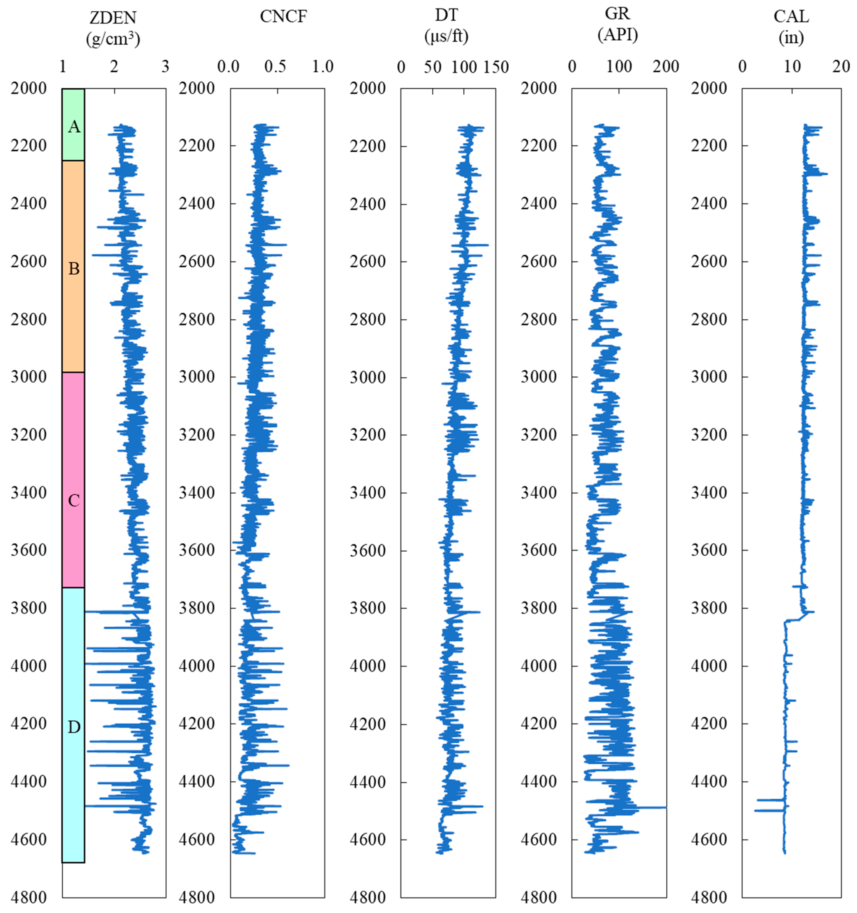
Data preprocessing is of great significance for obtaining accurate predictive models in machine learning. The learning samples in this study consist of input layer data and output layer data, where the input layer data come from the well logging data of the X-1 well, and the output layer data represent the formation pore pressure calculated using the Bowers method mentioned earlier. Based on previous research and field trial results, it has been shown that variables such as Acoustic Time-Difference (DT), Natural Gamma Ray (GR), Formation Density (ZDEN), Neutron Porosity (CNCF), and Borehole Diameter (CAL) can effectively reflect the variation of pore pressure. Therefore, these five well logging data variables are chosen as the input layer variables. The preprocessing of the original well logging data mainly involve tasks such as smoothing and filtering the well logging data, supplementing missing values, and replacing or removing abnormal data points.
As shown in
Figure 12, after data preprocessing, the depth range of the research interval in this study is from 2125 m to 4647 m, with each meter interval representing a row of learning sample data, totaling 2424 rows of data. Regarding data partitioning, this study randomly split the dataset into a training set and a testing set in an 8:2 ratio, and also set up a tenfold cross-validation set. Another partitioning method involves using 80% of the upper formation data as the training set and the remaining 20% of the lower formation data as the validation set. However, this method is not applicable to the X-1 well due to the majority of the lower formation being high-pressure formations, with a pore pressure equivalent density ranging from 1.2 g/cm
3 to 1.49 g/cm
3, while most of the upper formation maintains a pore pressure equivalent density of around 1.0 g/cm
3. If a model trained on the upper normal-pressure section is used to predict the pore pressure of the lower high-pressure section, it would result in significant errors, as the model has not learned from the data of the high-pressure section.
3.4.2. Model Establishment and Evaluation
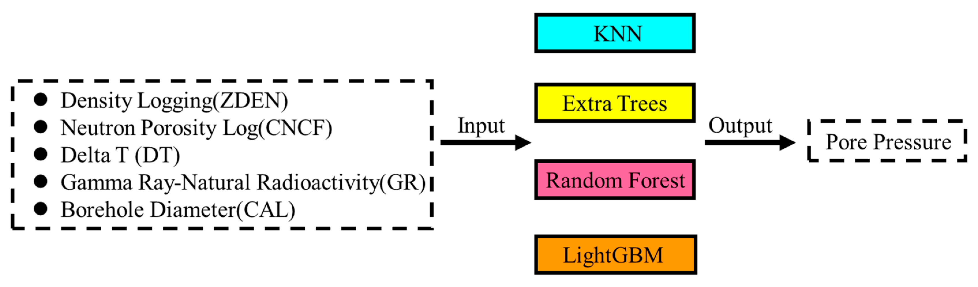
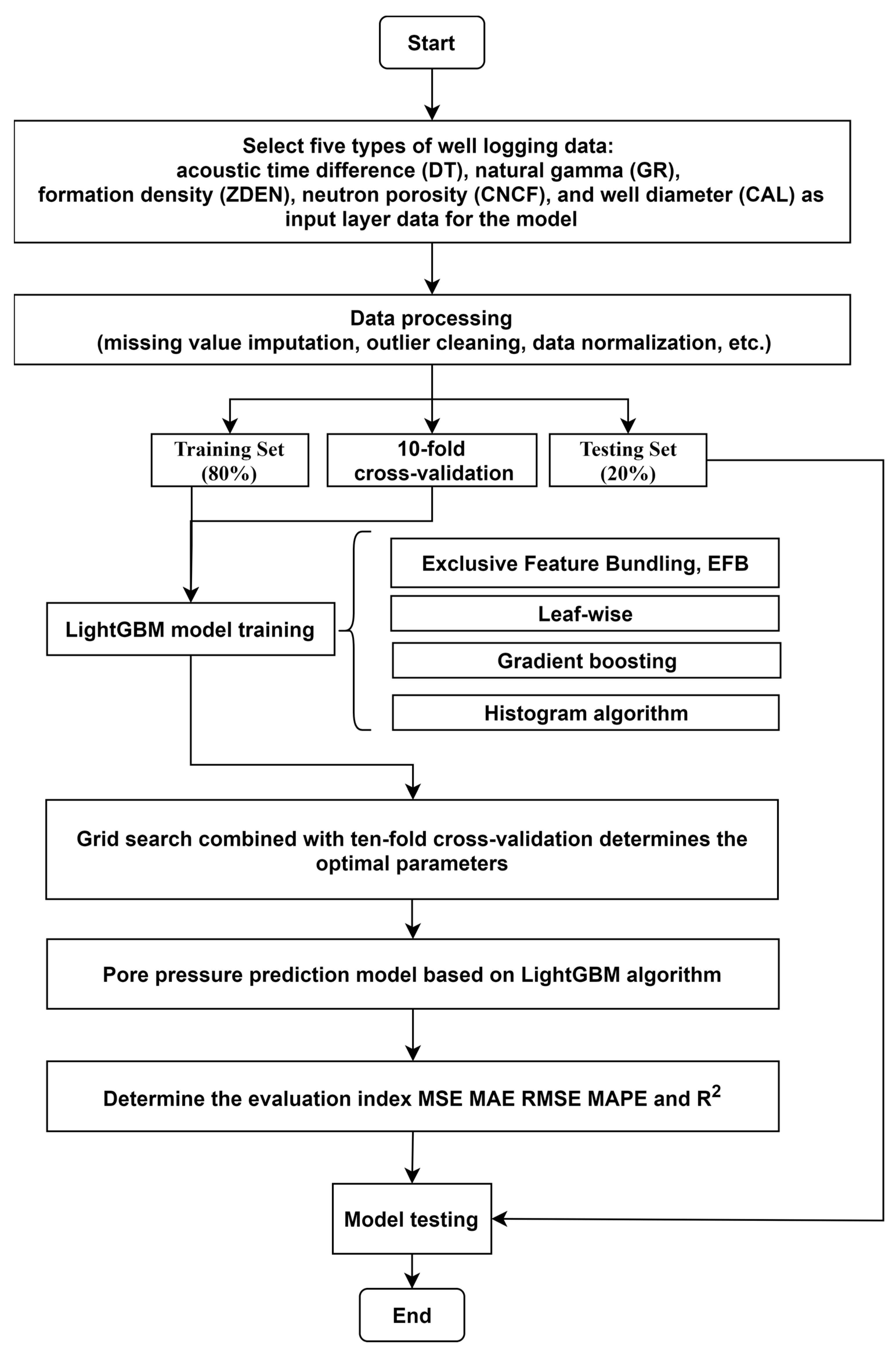
This paper constructs an intelligent pore pressure prediction model based on four machine learning algorithms: KNN, Extra Trees, Random Forest, and LightGBM. The feature importance is then calculated using the established regression models. The model’s structural overview is depicted in
Figure 13. The article employs the LightGBM algorithm model as an illustrative example to introduce the detailed procedural diagram of its construction, illustrated in
Figure 14.
The term “hyperparameters” pertains to the predetermined parameters defined prior to commencing the training of a machine learning model. These parameters wield a substantial influence over the predictive accuracy of the model. As hyperparameters cannot be learned through training, this study amalgamates theoretical insights and practical expertise to initially calibrate the ranges of hyperparameters employed across the four selected algorithmic models, thereby ascertaining their approximate scopes. Subsequent to confirming these ranges, a more precise refinement is conducted to narrow them down. After refining the ranges for individual hyperparameters, while considering the cumulative effects and utilizing evaluation metrics as benchmarks, the optimal values for each respective hyperparameter are ascertained. The hyperparameters for the four machine learning models are presented in
Table 2,
Table 3,
Table 4 and
Table 5.
Evaluation metrics for the four models on the cross-validation set, training set, and testing set are shown in
Figure 15. The predictive performance of different algorithm models is quantified using five metrics: Mean Squared Error (MSE), Root-Mean-Squared Error (RMSE), Mean Absolute Error (MAE), Mean Absolute Percentage Error (MAPE), and Coefficient of Determination (R
2). The physical meanings and calculation formulas of these evaluation metrics are as follows:
(1) MSE (Mean Squared Error): It is the expected value of the squared difference between the predicted values and the actual values. A smaller value indicates higher model accuracy.
(2) RMSE (Root-Mean-Square Error): It is the square root of MSE. A smaller value indicates higher model accuracy.
(3) MAE (Mean Absolute Error): It is the average of the absolute errors and reflects the actual prediction error. A smaller value indicates higher model accuracy.
(4) MAPE (Mean Absolute Percentage Error): It is a variation of MAE expressed as a percentage. A smaller value indicates higher model accuracy.
(5)
R2 (R Squared): It measures how well the predicted values compare to the case where only the mean is used. A value closer to 1 indicates higher model accuracy.
where
n is the number of samples,
xi is the actual value,
is the predicted value,
is the means of the actual value, and
is the means of the predicted value.
From
Figure 15, it can be observed that compared to the other three models, the KNN model performs the worst in all five evaluation metrics. On the other hand, the Extra Trees model, Random Forest model, and LightGBM model, which are all ensemble learning algorithms based on decision trees, outperform the KNN model in all evaluation metrics on the training set, testing set, and cross-validation set. Among these three models, the Extra Trees model shows relatively poor performance compared to the Random Forest model and LightGBM model, with LightGBM model performing the best. Regarding the training duration, the Random Forest model takes the longest time, with a duration of 2.522 s. The Extra Trees model comes next, taking 1.3 s. The KNN model has the shortest training time, only 0.067 s, while the LightGBM model takes 0.54 s. Overall, despite the KNN model having the shortest training time, its performance in all evaluation metrics is the worst. Therefore, it is preliminarily determined that the LightGBM model exhibits the best overall performance.
As the testing set is used to evaluate the performance of the finally selected optimal model, this study focuses on the performance of the four models on the testing set in terms of various evaluation metrics. As shown in
Table 6, the LightGBM model achieves the following five evaluation metrics on the testing set: 0.006 (MSE), 0.078 (RMSE), 0.04 (MAE), 3.419 (MAPE), and 0.647 (R
2). Compared to the LightGBM model, the KNN model, Extra Trees model, and Random Forest model show increases in errors on the testing set for MSE by 83.333%, 33.333%, and 16.667%, respectively. For RMSE, the errors increase by 33.333%, 14.103%, and 5.128%, respectively. The MAE errors increase by 32.5%, 20%, and 2.5%, respectively. Additionally, the MAPE errors increase by 34.016%, 19.596%, and 0.643%, respectively. However, in terms of R
2, the errors decrease by 43.122%, 20.711%, and 15.765%, respectively.
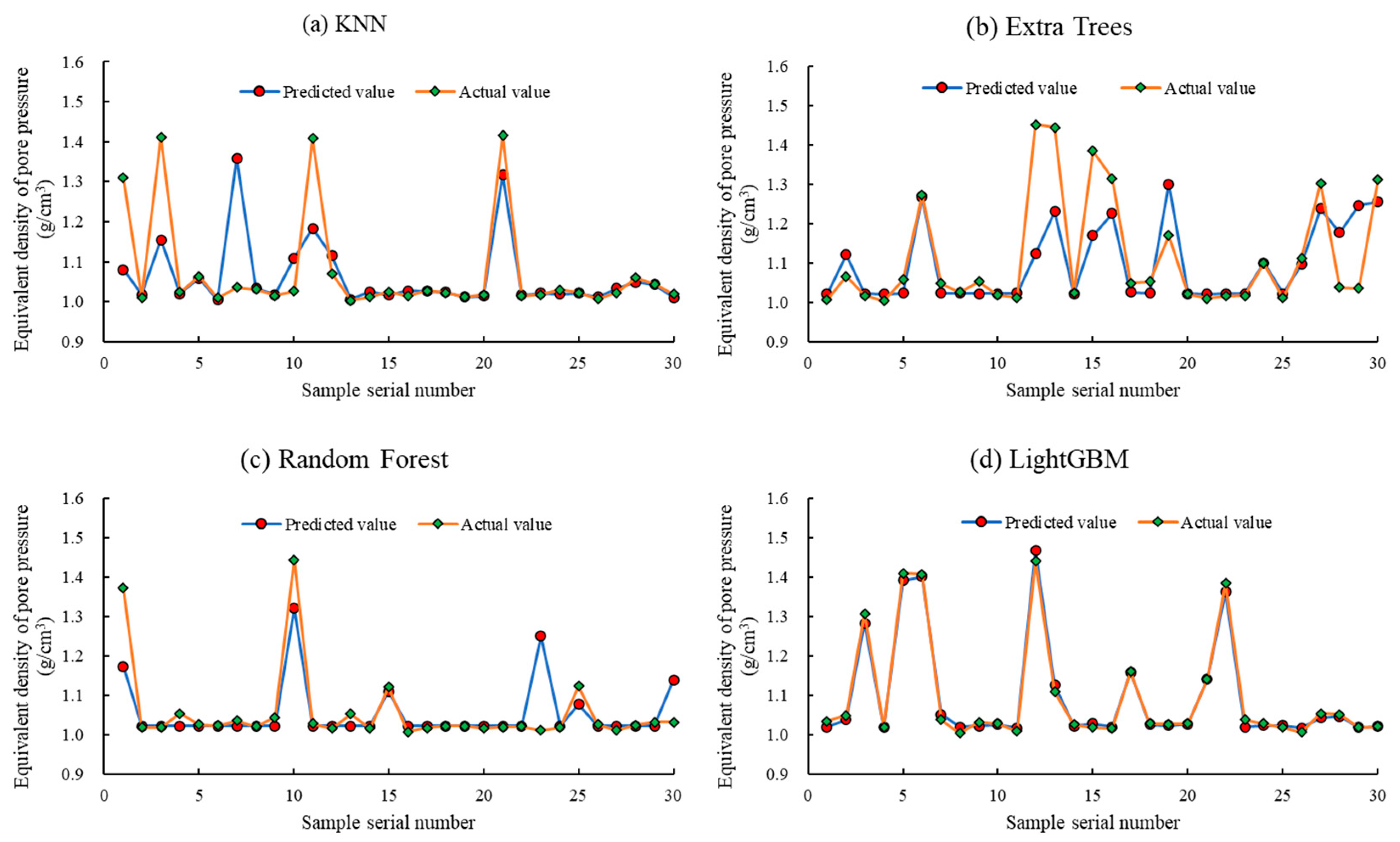
We randomly selected 30 predicted values from each of the four algorithm models on the testing set and compared them with the actual values, as shown in
Figure 16. Firstly, it is evident that the KNN model and Extra Trees model exhibit significant deviations in some predicted values from the actual values, performing notably worse than the Random Forest model and LightGBM model. Secondly, for the data points corresponding to normal pressure, the predicted values of all four models align well with the actual values. However, for the data points corresponding to high pressure, only the LightGBM model performs well, while the other three models show unsatisfactory results. Although the Random Forest model seems to perform relatively well overall, a closer inspection in
Figure 16c reveals that out of the 30 randomly selected data points, 24 points have the same predicted result, which is 1.022. This means that the red data points representing the predicted values show minimal fluctuations. In the entire set of 485 testing data points, the value 1.022 appears a total of 326 times, accounting for a high proportion of 67.216%. This indicates that the Random Forest model has become ineffective in making accurate predictions.
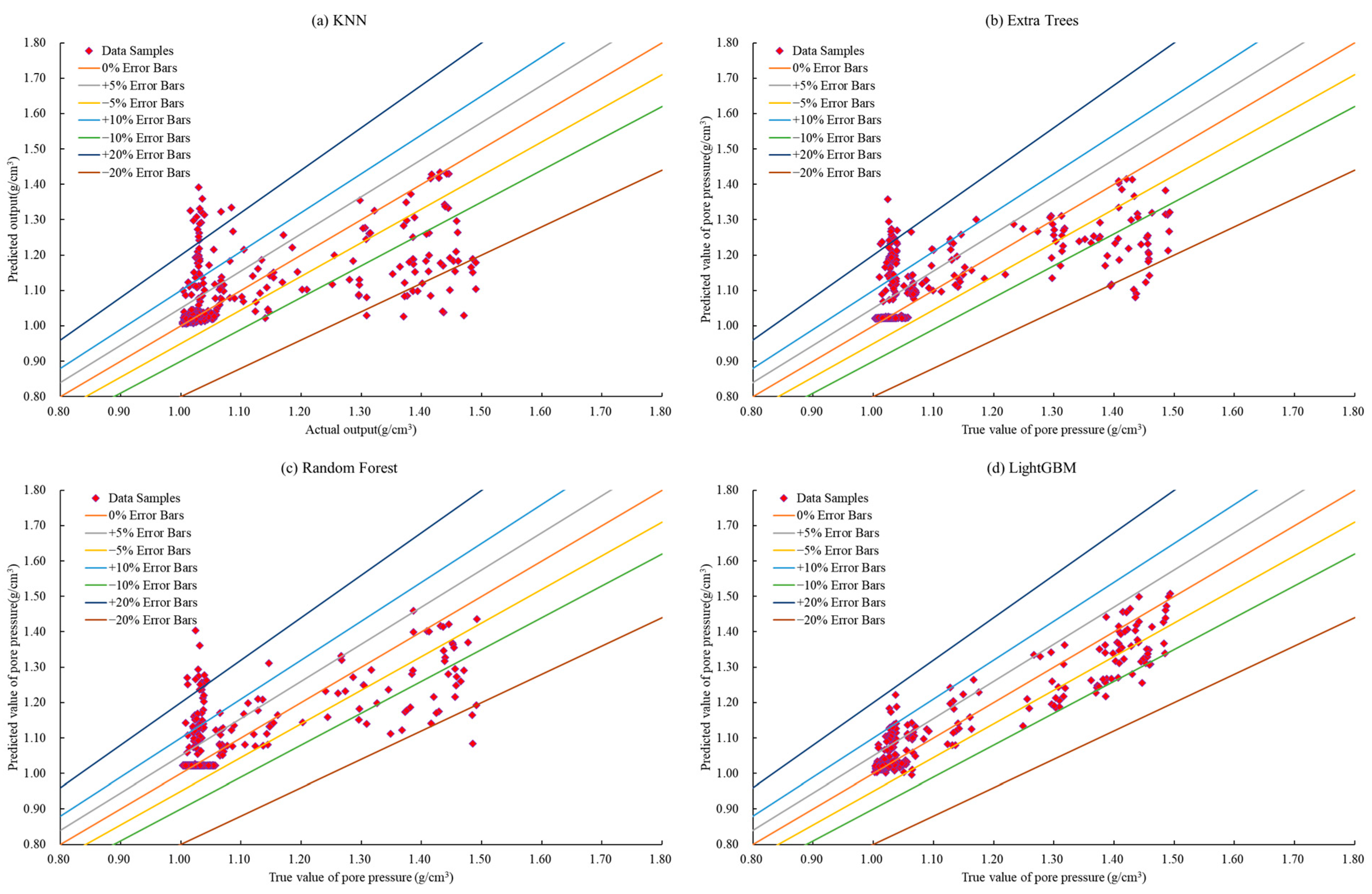
Figure 17 illustrates the distribution of prediction errors for the four models on the testing set. From
Figure 17, it is evident that the LightGBM model performs the best. Except for a few data points with errors between 10% and 20%, the majority of the points have prediction errors concentrated within the range of −10% to +10%. On the other hand, the other three models show a significant number of data points with prediction errors exceeding 10% and even 20%. Another notable feature is that all four models demonstrate relatively good prediction accuracy for data points corresponding to normal pressure. However, for data points corresponding to high pressure, the errors significantly increase, which is consistent with the conclusion drawn from
Figure 16.
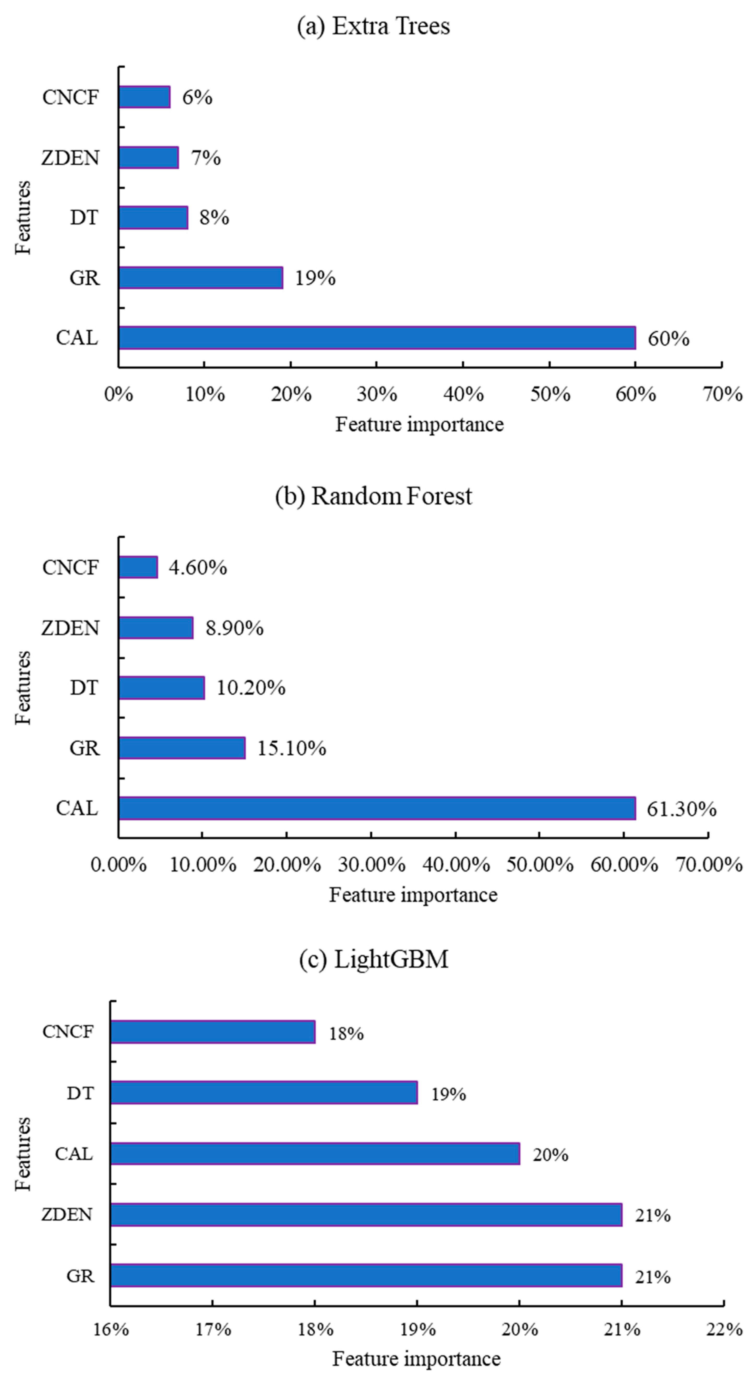
Feature importance can measure the contribution of each input feature to the model’s prediction results, highlighting the correlation between different input variables and the prediction target. Additionally, decision tree-based models can be used to evaluate feature importance, while the KNN model cannot. Therefore, this study calculated the feature importance of the Extra Trees model, Random Forest model, and LightGBM model, as shown in
Figure 18. From
Figure 18, it is evident that the feature importance distribution of the Extra Trees model and Random Forest model is highly consistent. For both models, the five input features are ranked in descending order of feature importance as CAL, GR, DT, ZDEN, and CNCF, with nearly identical values for each input feature. CAL has a significant impact on the predictions of the Extra Trees model and Random Forest model, accounting for more than 60% of the feature importance. This can explain why these two models have relatively large prediction errors for data points corresponding to high pressure. During model training, most of the data points used were for normal-pressure conditions, with a CAL value of approximately 12.25 inches. However, the data points corresponding to high pressure came from deep formations, where a drill bit with a diameter of 8.5 inches was used, resulting in a CAL value of around 8.5 inches (as shown in
Figure 12). Since the Extra Trees model and Random Forest model are heavily influenced by the CAL input feature, other input variables cannot effectively constrain the models, leading to their inability to predict high-pressure data points accurately. On the other hand, the LightGBM model shows that the feature importance of the five input variables is similar, all around 20%. This indicates that the LightGBM model can adequately consider each input variable, reducing the likelihood of significant prediction biases and significantly improving prediction accuracy. In conclusion, the LightGBM model performs exceptionally well among the four models, with high prediction accuracy, strong generalization ability, and short training time. Therefore, this study utilizes the well-trained LightGBM model to predict the neighboring well’s porosity pressure for the X-1 well.
3.4.3. Pore Pressure Prediction Results
Around well X-1, three other wells, namely, X-2 and X-3, are situated in close proximity. The X-2 well is about 6.7 km southwest of X-1, and the X-3 well is approximately 1.4 km away from X-1, as depicted in
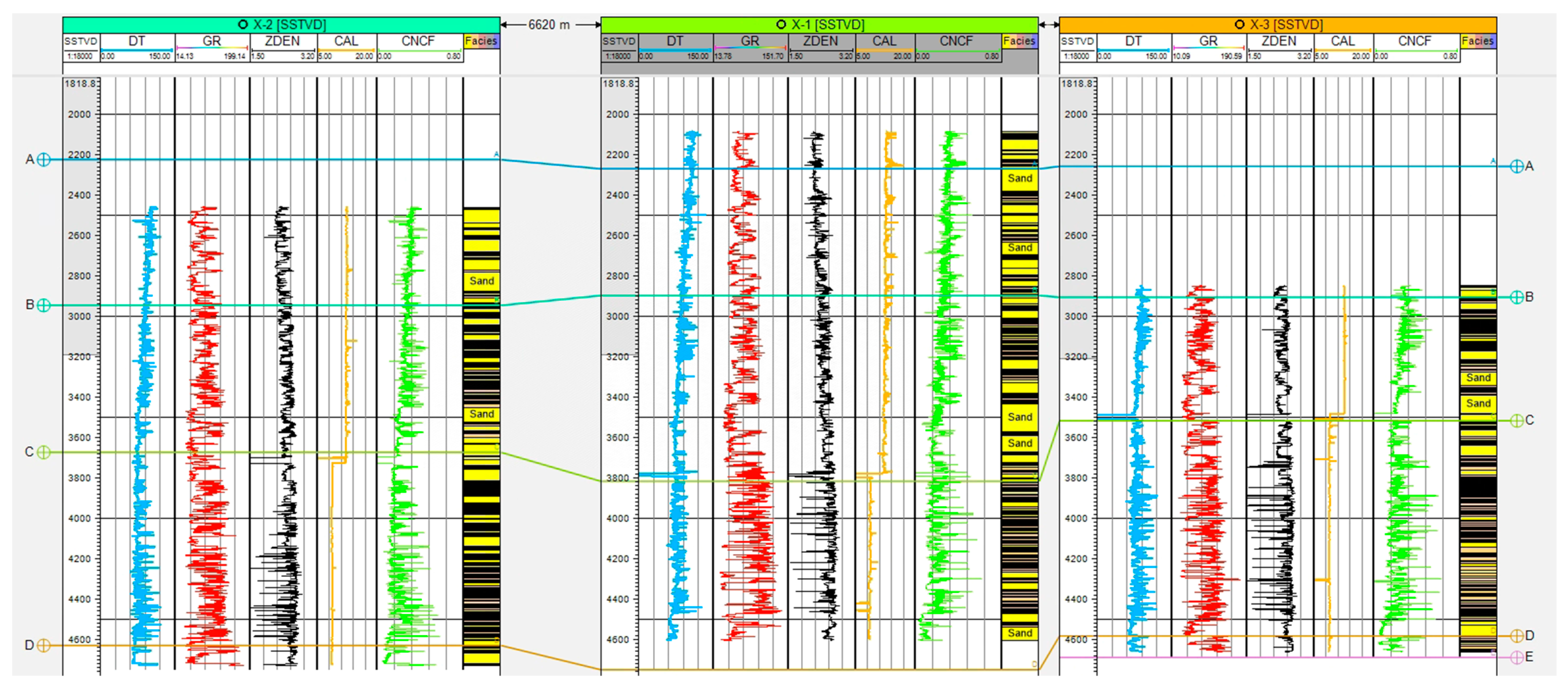
Figure 19. The input layer data from the wells, including delta t (DT), gamma logging (GR), formation density logging (ZDEN), neutron porosity logging (CNCF), and borehole diameter (CAL), have been preprocessed for subsequent analysis.
Figure 20 displays a comparison of input layer data for the wells X-2 and X-3. Subsequently, the preprocessed data for these wells are utilized as input for the trained LightGBM model, which predicts the pore pressure. The predicted results are illustrated in
Figure 21, while
Figure 22 presents the actual measured pore pressure for all three wells in the X-block.
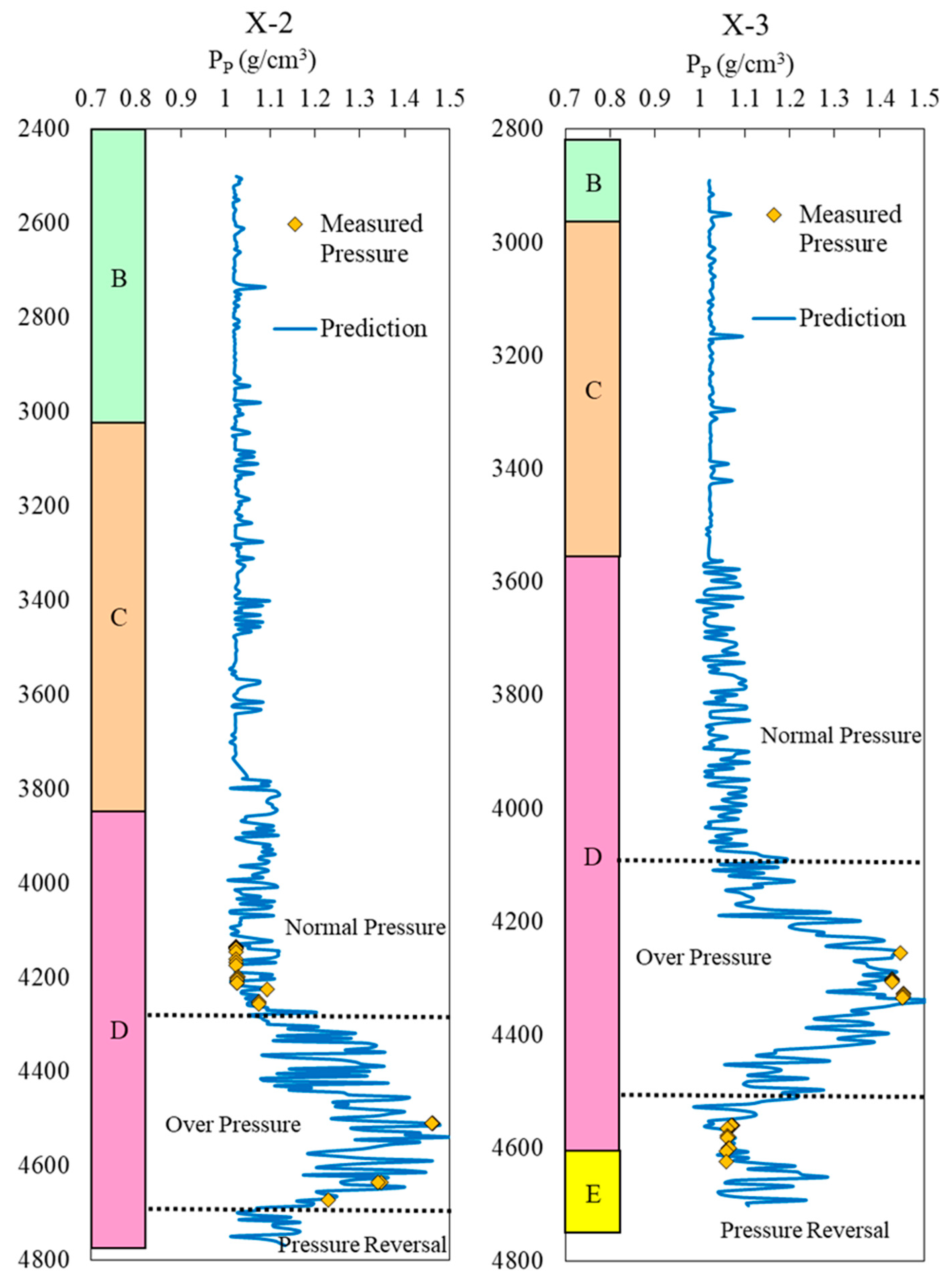
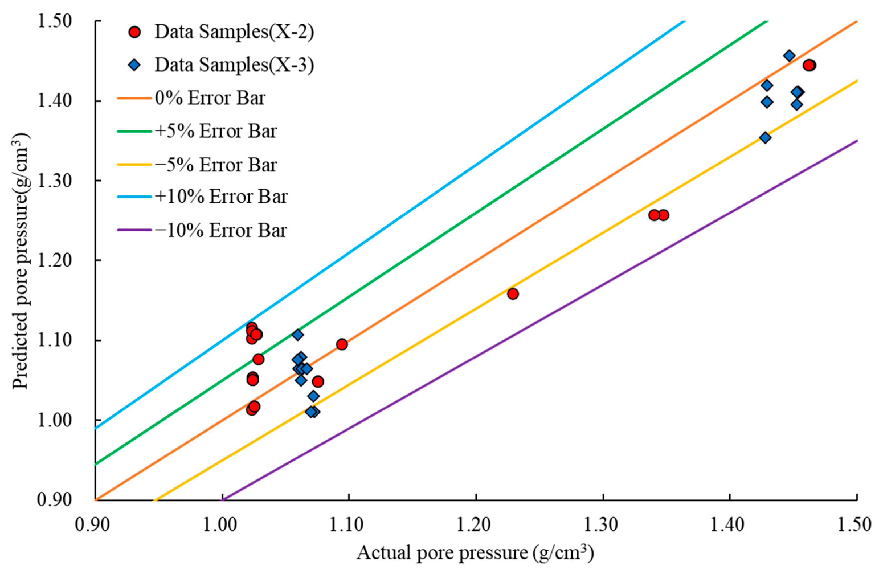
The results from
Figure 21 indicate a strong consistency between the predicted pore pressure values of wells X-2 and X-3 and that of well X-1. As for the stratigraphy, all three wells exhibit normal pressure in the upper part of the B formation, C formation, and D formation. The high-pressure system primarily develops in the middle and lower parts of the D formation. Moreover, with increasing depth, the pressure exhibits a “step-like” increase. Preliminary findings suggest that the “step-like” distribution of pore pressure in the strata is associated with lithology and stratigraphy. In general, pressure steps occur beneath thick mudstone layers that are rich in coal seams, and this pressure distribution aligns with the characteristics of mature source rocks. Regarding depth, the X-2 well enters the high-pressure section at approximately 4300 m, while the X-3 well does the same at around 4100 m. Simultaneously, the X-2 and X-3 wells both encounter the pressure reversal section in the lower part of the D formation, at depths of around 4678 m and 4516 m, respectively.
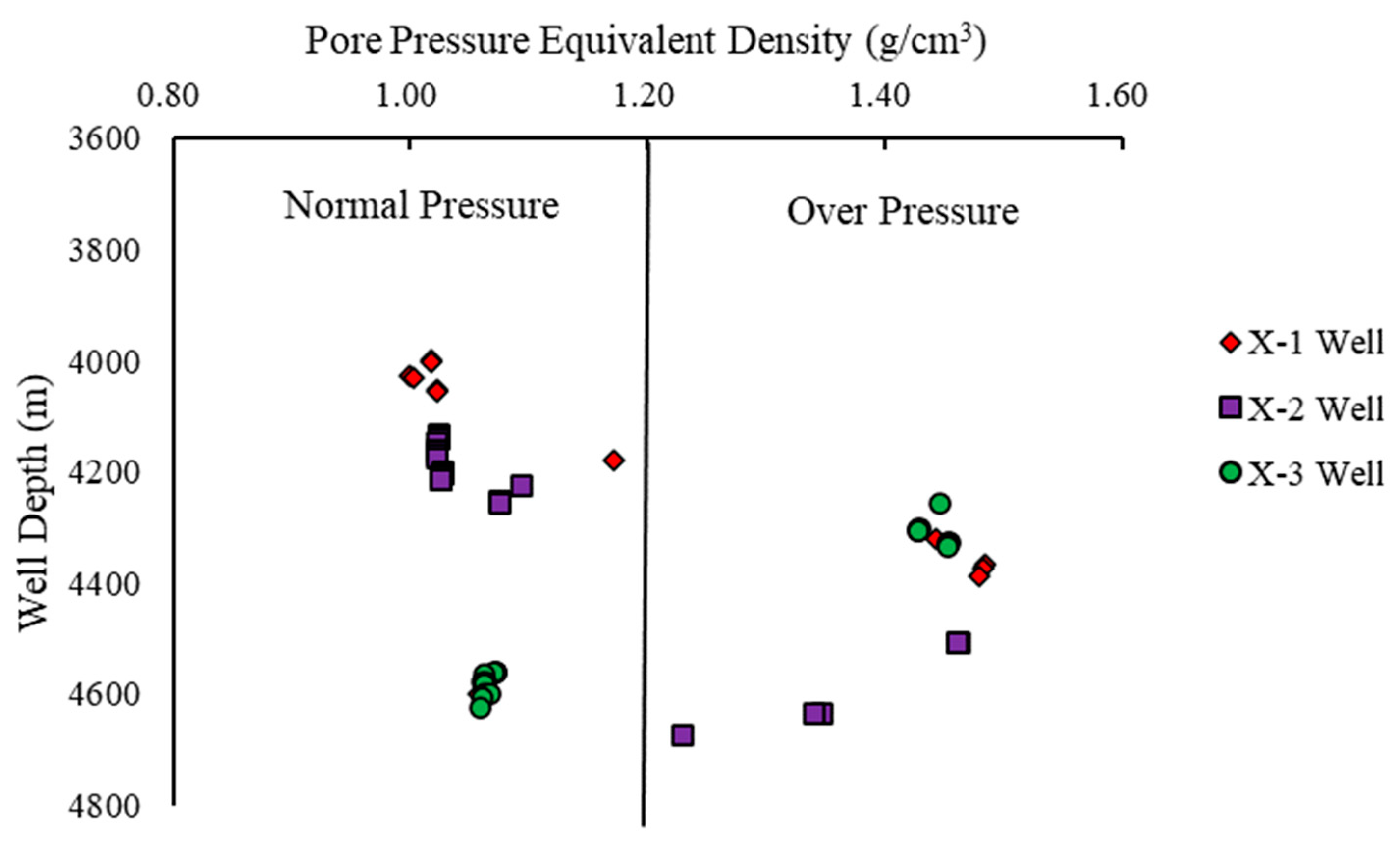
The combination of
Figure 21,
Figure 22 and
Figure 23 reveals that the measured pore pressure data for wells X-1, X-2, and X-3 includes both normal- and high-pressure data points. The highest measured pore pressure value is 1.463 g/cm³, observed in the X-2 well at a depth of 4508.21 m. The predicted pore pressure values obtained from the LightGBM model for wells X-2 and X-3 exhibit excellent agreement with the measured values. The prediction error for the X-2 well ranges from −6.676% to 9.166%, and for the X-3 well, it ranges from −5.803% to 4.438%. The model’s overall prediction accuracy surpasses 90%, indicating its ability to establish a complex nonlinear mapping relationship between the five sets of well logging data used as input variables and the formation pore pressure. This showcases the model’s high prediction accuracy, excellent generalization capability, and overall reliability.
In summary, the conventional approach to pore pressure calculation using fixed mathematical formulas entails complex parameter fitting and correction procedures. However, it is ill-suited for regions with sparse data, recently established geological blocks, or blocks characterized by intricate geological conditions. The suggested approach for predicting pore pressure in blocks with anomalously high pressure, utilizing machine learning algorithms, is viable, with the LightGBM model exhibiting optimal performance. This study introduces an intelligent process for predicting pore pressure, specifically designed for such high-pressure blocks. It integrates an analysis of pore pressure generation mechanisms with the development of a machine learning-based predictive model. This comprehensive approach substantially improves the precision of pore pressure prediction, providing valuable guidance for on-site optimization of wellbore structures and drilling fluid performance. By eliminating subjective human influences and conserving resources, it emphasizes the significance of employing artificial intelligence to predict formation pore pressure. This highlights a pivotal avenue for future research.
3.5. Discussions
The study area is situated within a characteristic anomalous high-pressure zone, characterized by notably elevated pressures in the deeper strata. The pore pressure coefficient can attain a maximum value of 1.6. The limited safe range of drilling fluid density poses substantial on-site well control risks. Furthermore, substantial variations in pore pressure distribution exist both vertically and horizontally across this zone due to structural controls. The origination point of abnormally high pressure exhibits unpredictable variation, rendering the precise characterization of strata pressure challenging. The complexities described render conventional pore pressure prediction methods ill-suited.
Accordingly, this study utilizes machine learning methodologies. Four machine learning algorithms, namely, KNN, Extra Trees, Random Forest, and LightGBM, are chosen to formulate an advanced model for predicting pore pressure. The findings demonstrate that the LightGBM model excels in overall performance. The actual error in pore pressure prediction is within the range of ±10%, satisfying the precision criteria for on-site strata pore pressure prediction. This furnishes valuable reference data to enhance drilling safety within this zone. To seamlessly integrate the research findings into on-site drilling operations, the following recommendations are put forth:
(1) To predict anomalous high-pressure layers, monitor strata pressure during drilling operations. Upon encountering abnormally high pressure, assess the load-bearing capacity of the upper strata. If deemed viable, conduct pre-emptive pressure-bearing experiments; otherwise, terminate ongoing drilling before penetrating the high-pressure layer. Implement cement sealing and adjust drilling fluid density prior to entering this stratum. During the cementing process, substitute drilling fluid with cement slurry to avert undue pressure differentials that could impact the single check valve in the float collar and shoe.
(2) To ensure drilling safety, it is advised to employ pressure control apparatuses for accurate and efficient regulation of the equivalent circulating density (ECD) of downhole drilling fluid. Given the intricate nature of sand and mud formations in this well region, along with hydrocarbon-bearing source rocks, stabilize the bottom hole ECD during pipe connections and tripping by manipulating backpressure and overseeing the injection and substitution of dense mud. This safeguards against wellbore instability arising from pressure oscillations during such operations. In instances where a substantial gas discharge coincides with the anomalous high pressure, contemplate the use of gas-tight connectors for the casing.
(3) To incorporate the pore pressure forecasts generated by the machine learning model into the established systems and apparatuses on the drilling site, precise geological and engineering data organization is paramount. Embed the model within the extant system and fashion software interfaces to relay real-time drilling data to the model, subsequently exhibiting the model’s prognostications within the field system. Ultimately, validate the coherence between the model’s predictions and actual data, thus upholding the safety and stability of system performance. Instruct on-site personnel in model utilization and sustain vigilant oversight to enhance its efficacy. This comprehensive endeavor mandates the contemplation of diverse facets, encompassing data, software, and hardware realms, necessitating collaboration with experts in pertinent domains to facilitate a seamless integration process aligned with on-site requisites.
4. Conclusions
The current research on utilizing machine learning for predicting formation pore pressure presents two prominent issues. Firstly, it lacks the integration of an analysis of the formation’s compaction mechanism as a starting point for pore pressure prediction. Secondly, the application of machine learning methods for predicting pore pressure in abnormal high-pressure areas remains an unexplored research area. In light of these limitations, this paper addresses these concerns by proposing a comprehensive machine learning-based method for predicting pore pressure in abnormal high-pressure areas, taking into account the specific engineering background of X-block. The primary conclusions of this study are as follows:
(1) Considering the geological background of well X-1 and the specific conditions near the well, this study establishes a notable link between hydrocarbon generation, overpressure, and the emergence of abnormal high pressure in the deep formations of the target well. By utilizing well logging data from X-1, the study employs two complementary method, Bowers’ method and the density–sonic velocity crossplot method, to analyze the origin of abnormal high pressure in the deep formations of X-1. The investigation concludes that the primary objective interval, i.e., the middle-lower section of the D Formation, has reached the hydrocarbon generation threshold. Furthermore, the substantial amount of oil and gas produced by hydrocarbon generation serves as the primary cause of abnormal high pressure in the lower formations.
(2) After determining the overpressure genesis in X-block, the Bowers’ method was chosen to predict the pore pressure of well X-1. Based on the magnitude of the pore pressure, X-1’s entire wellbore was divided into three distinct sections: normal-pressure, high-pressure, and pressure reversal sections. Notably, the high-pressure section exhibited a conspicuous step-like increase in pressure, with the boundary between the normal- and high-pressure sections identified at 4190 m in the middle section of the D Formation. Additionally, the boundary between the high-pressure and pressure reversal sections was discovered at 4520 m in the lower section of the D Formation. Upon comparing the predictions with the actual measured pore pressure data, it was found that all prediction errors were less than 5%. This observation underscores the significance of subdividing the wellbore into smaller intervals, focusing on analyzing the genesis mechanism of the abnormal-pressure sections, and selecting appropriate pore pressure prediction methods. Consequently, these approaches have substantially improved the accuracy of pore pressure prediction.
(3) Utilizing a meticulous examination of five carefully chosen well logging datasets and employing four distinct machine learning algorithms, we have constructed an intelligent predictive model for pore pressure. The effectiveness of these four models is then meticulously compared and assessed using a set of five diverse evaluation metrics, which incorporates the Mean Squared Error (MSE). The findings revealed that the LightGBM model exhibited superior performance, characterized by both a significantly shorter training time (0.54 s) and exceptional overall performance. The evaluation metrics for the LightGBM model on the test dataset were as follows: MSE of 0.006, RMSE of 0.078, MAE of 0.04, MAPE of 3.419, and R2 of 0.647. These values signified substantial performance enhancement when contrasted with the remaining three models. In order to bolster the validation of this model’s applicability within the X block, the LightGBM model was employed to forecast the pore pressure of two neighboring wells (X-2 and X-3) in close proximity to well X-1. A comparison against the actual measured pore pressure data revealed a predicted error range of −6.676% to 9.166% for well X-2 and −5.803% to 4.438% for well X-3. This observation underscores the LightGBM model’s capability to accurately predict reservoir pore pressure within the X block. Such accurate predictions offer valuable reference data for the assurance of drilling safety in the specified area.


 ,
, 


