Numerical Simulation of Flashing Flows in a Converging–Diverging Nozzle with Interfacial Area Transport Equation

Abstract

Flashing flows of initially sub-cooled water in a converging–diverging nozzle is investigated numerically in the framework of the two-fluid model (TFM). The thermal non-equilibrium effect of phase change is considered by an interfacial heat transfer model, while the pressure jump across the interface is ignored. The bubble size distribution induced by nucleation, bubble growth/shrinkage, coalescence, and breakup is described based on the interfacial area transport equation (IATE) and constant bubble number density model (CBND), respectively. The results are compared with the experimental data. Satisfactory prediction of the axial pressure distribution along the nozzle as well as the flashing inception, is achieved by the TFM-IATE coupling method. It was also found that the vapor production in the diverging section was overpredicted, and the radial gas volume fraction distribution deviated from the experiment. The radial diameter profiles exhibit opposite patterns at the nozzle throat and near the outlet, and similar trends can be observed for the superheated degree. A poly-disperse method is suggested to be introduced to describe the evolution of interfacial area concentration.

1. Introduction

Flashing occurs when the pressure of a liquid rapidly decreases below the saturation pressure at a given temperature [1]. Flashing flow has been widely used in industrial production and can be divided into three categories based on the corresponding technical principles: (1) separating liquid phase and heterogeneous substances, such as multi-stage flashing technology for seawater desalination [2]; (2) flashing spray technology to improve spray performance, e.g., cooling high-power equipment or improving fuel combustion characteristics [3]; and (3) converting thermal energy to other forms of energy, such as using steam from flashing to drive steam turbines to generate electricity in geothermal power plants [4].

Flashing also occurs in the event of damage or leakage of cooling pipes, pressure pipes, and other equipment [5]. The Loss of Coolant Accident (LOCA) is a particularly common type of accident in nuclear power plants, wherein a rupture of the pipe causes a reduction in the coolant load of the circuit [6]. Due to the high-temperature and high-pressure conditions of the first circuit, a large amount of coolant and steam are released from the breach when flashing occurs, forming a complex gas–liquid two-phase flow. In the event of a LOCA, the loss of coolant can lead to core bareness or even meltdown, while the radioactive material brought out by the coolant can increase environmental radiation dose, thus posing a threat to public safety. Therefore, studying the flashing flow in high-temperature and high-pressure pipelines to predict the gas–liquid two-phase flow, heat transfer and mass transfer behaviors are of great significance for ensuring the safe operation of nuclear power plants.

In the flashing process, several significant sub-phenomena are involved, such as nucleation, bubble growth, bubble coalescence, and breakup [7]. These processes are affected by environmental pressure and temperature changes and are closely linked to the interphase heat transfer process. Coalescence and breakup are usually driven by interphase forces, whereas the nucleation and growth of bubbles provide an additional mechanism for bubble size evolution in flashing flow, which can then affect the energy and mass flow transport between phases by altering the interfacial area concentration and the flow conditions.

The advancement of computer technology has enabled Computational Fluid Dynamics (CFD) to become a crucial tool for studying the flashing flow [8]. For large-scale flashing scenarios [9,10], the Two-Fluid Model (TFM) has an advantage in balancing the computational efficiency and accuracy. For TFM flashing simulation, the interfacial area concentration is an essential parameter of the interphase transfer model and is significantly impacted by nucleation, bubble growth, coalescence, and breakup. Commonly used interfacial area concentration models include the Constant Bubble Diameter (CBD) Model [11,12], the Constant Bubble Number Density (CBND) Model, the Bubble Number Density Transport Equation [13,14], the Interfacial Area Transport Equation (IATE) [15], and the Population Balance Model (PBM) [16]. The first two models are quite simple in implementation and utilization, but they are only suitable when the bubble size or number density does not change significantly. PBM can accurately capture the evolution of interfacial area concentration, though more computational resources are required as the number of size classes increases. In contrast, IATE is a monodisperse method with relatively high efficiency and can take into account several factors that affect the area concentration in the source terms of the equation. Despite this, IATE has seen less application in numerical simulations of flashing flow. This paper thus uses IATE to simulate the evolution of interfacial area concentration during flashing and explore its influence on multiphysics distribution.

2. Mathematical Model

2.1. Two-Fluid Model

The transport equations of TFM with source terms for interfacial mass, momentum, and heat exchanges are represented below.

$$\frac{\partial \left({\alpha }_k{\rho }_k\right)}{\partial t}+\nabla \cdot \left({\alpha }_k{\rho }_k{u}_k\right)={\Gamma }_k$$

(1)

$$\begin{array}{l}\frac{\partial \left({\alpha }_k{\rho }_k{u}_k\right)}{\partial t}+\nabla \cdot \left({\alpha }_k{\rho }_k{u}_k{u}_k\right)\\ =-{\alpha }_k\nabla p+\nabla \cdot \left\{{\alpha }_k{\mu }_{\mathrm{eff},k}\left[\left(\nabla u_k+{\left(\nabla u_k\right)}^{\mathrm{T}}\right)-\frac{2}{3}\left(\nabla \cdot u_k\right)I\right]\right\}\\ +{\alpha }_k{\rho }_{k}g+\left({\Gamma }_{kj}{u}_j-{\Gamma }_{jk}{u}_k\right)+F_k\end{array}$$

(2)

$$\begin{array}{l}\frac{\partial \left({\alpha }_k{\rho }_k{H}_k\right)}{\partial t}+\nabla \cdot \left({\alpha }_k{\rho }_k{H}_k{u}_k\right)+\frac{\partial \left({\alpha }_k{\rho }_k{K}_k\right)}{\partial t}+\nabla \cdot \left({\alpha }_k{\rho }_k{K}_k{u}_k\right)\\ =-{\alpha }_k\frac{\mathrm{d}p}{\mathrm{d}t}+\nabla \cdot \left({\alpha }_k{D}_{\mathrm{eff},k}\nabla H_k\right)+Q_k\end{array}$$

(3)

where α, ρ, u, p, H, and K are volume fraction, density, velocity, pressure, enthalpy, and kinetic energy, respectively. Subscript k = g, l represents gas and liquid phases, respectively. Sources terms Γ, F, and Q in the transport equations determine the interfacial exchanges and require closure models. It is stressed that the following closure models are based on the assumptions of spherical vapor bubbles and bubbly flow regime.

2.2. Main Closure Models

During the flashing process, the interfacial mass transfer occurs through three distinct mechanisms, nucleation, inertia-controlled phase change, and thermal-controlled phase change [17,18]. With the assumption of pressure equilibrium across the interface, we can neglect the inertial-controlled terms. Therefore, the interfacial mass transfer can be expressed as follows:

$${\Gamma }_{\mathrm{g}}=-{\Gamma }_{\mathrm{l}}={\Gamma }_{\mathrm{N}}+{\Gamma }_{\mathrm{T}}$$

(4)

where Γ_N and Γ_T represent mass transfer rate arising from nucleation and heat transfer, respectively.

Since the superheat degree in flashing flows is relatively low, we can ignore the contribution from a homogeneous nucleation [13]. Additionally, it is important to note that heterogeneous nucleation can be classified into two types, bulk nucleation and wall nucleation. In the present study, we have chosen to omit the consideration of bulk nucleation. This is performed in order to avoid introducing uncertainties related to adjustable parameters such as the heterogeneous factor and the number density of nucleation site in the bulk fluid [18]. As a result, the mass source term due to wall nucleation can be expressed as follows:

$${\Gamma }_{\mathrm{N}}=\frac{\mathsf{\pi }{d}_{\mathrm{dep}}^3}{6}{\rho }_{\mathrm{g}}{J}_{\mathrm{HET},\mathrm{w}}\frac{S_{\mathrm{f}}}{V_{\mathrm{c}}}$$

(5)

where d_dep is bubble departure diameter; S_f the surface area of the wall where nucleation occurs; V is the volume of the cells adjacent to the wall, and J_HET,w is wall nucleation rate given by the Shin–Jones model [19]:

$$J_{\mathrm{HET},\mathrm{w}}=f_{\mathrm{dep}}{N}_{\mathrm{N}}=2.5\times {10}^{-4}{\left(T_{\mathrm{l}}-T_{\mathrm{sat}}\right)}^3\frac{r_{\mathrm{dep}}^2}{r_{\mathrm{c}}^4}$$

(6)

where f_dep is departure frequency, N_N nucleation site density, T_sat saturation temperature, and r_dep and r_c are departure radius and critical radius, respectively.

During the thermal-controlled phase change stage, the growth and shrinkage of the bubble are determined by the temperature difference between the gas and liquid phases. It is assumed that the gas phase and gas–liquid interface are at the saturation condition corresponding to the local pressure; then, ${\Gamma }_{\mathrm{T}}$ is given as follows:

$${\Gamma }_{\mathrm{T}}=\frac{\left[h_{\lg }{A}_{\mathrm{i}}\left(T_{\mathrm{i}}-T_{\mathrm{l}}\right)\right]}{H_{\mathrm{il}}-H_{\mathrm{ig}}}$$

(7)

where A_i is the IAC which is discussed in the next section; the interface temperature, T_i, is maintained at the saturation temperature, and h_lg represents the heat transfer coefficient, which can be estimated by a variety of correlations available in the literature. For bubble growth cases, the Plesset–Zwick correlation [20] derived theoretically by considering the heat conduction between vapor bubbles and surrounding liquid is selected:

$$Nu=\frac{12}{\mathsf{\pi }}Ja$$

(8)

The classical Ranz–Marshall correlation [21] and Liao [22] correlation involving the effect of interfacial slip velocity and turbulence are chosen for simulating the flashing pipe flows.

$$Nu=2+0.6R{e}_{\mathrm{g}}^{1/2}P{r}_{\mathrm{l}}^{1/3}$$

(9)

$$Nu=\frac{12}{\mathsf{\pi }}Ja+\frac{2}{\sqrt{\mathsf{\pi }}}P{e}^{1/2}+\frac{2}{\sqrt{\mathsf{\pi }}}P{e}_{\mathrm{turb}}^{1/2}\frac{d_{\mathrm{g}}}{l_{\mathrm{turb}}}$$

(10)

where Ja is the Jakob number; Re the Reynold number; Pr is the Prandtl number; Pe is the Péclet number, and Pe_turb the turbulent Péclet number, respectively. l_turb is the turbulent characteristic length. It is stressed that the Plesset–Zwick correlation only considers the heat conducted from the nearby superheated liquid; the Ranz–Marshall correlation is established based on the experiments of spherical water drops and is validated in the range Re_g < 450 and Pr_l < 250; the Liao correlation combines heat conduction, convection, and turbulence effect by the way of linear accumulation.

The flow rate of latent and sensible heat transferring from the gas–liquid interface to phase k takes the following form:

$$Q_k={\Gamma }_{\mathrm{T}}{H}_{\mathrm{i}k}+h_{\lg }{A}_{\mathrm{i}}\left(T_{\mathrm{i}}-T_k\right)$$

(11)

The interfacial forces F_k denote the interaction between phases at their interface, and the drag force, lift force, wall force, and turbulent dispersion force are included in the present work. The gas phase is assumed to be laminar flow, while the turbulence in the liquid phase is obtained via the k-ω SST model. The Ma correlation [23] is introduced to describe the bubble-induced turbulence (BIT). All the closures for interfacial forces and turbulence are referred to the baseline model [24] and summarized in

Table 1. Closure models for the momentum equation.

Term		Reference
Interfacial force	Drag force	Ishii and Zuber [26]
	Lift force	Tomiyama et al. [27]
	Wall force	Hosokawa et al. [28]
	Turbulent dispersion force	Burns et al. [29]
	Virtual force	Constant virtual mass coefficient, Cvm = 0.5
Turbulence	Liquid	k-ω SST [30]
	BIT	Ma et al. [23]

. Due to the limited space, the reader is referred to Liao et al. [25] for more detailed information.

2.3. Interfacial Area Transport Equation

Ishii et al. [31,32] derived the IATE based on the Boltzmann Transport Equation, which can be divided into a One-Group Model [33] for bubbly flow and a Two-Group Model [34] for slug and churn-turbulent flow conditions. The One-Group IATE approximates bubbles as spherical and replaces the bubble diameter with the equivalent spherical volume diameter, while all bubbles in the group share the same interaction mechanism with the liquid phase. On the other hand, the Two-Group IATE separates spherical/distorted bubbles into one group and cap/slug bubbles into another, requiring the construction of a separate interphase interaction model for each group [35].

This paper focuses on flash flow dominated by bubble flow, so the One-Bubble Group IATE model is given as follows:

$$\frac{\partial A_{\mathrm{i}}}{\partial t}+\nabla \cdot \left(A_{\mathrm{i}}{u}_{\mathrm{i}}\right)=\frac{1}{3\phi }{\left(\frac{{\alpha }_{\mathrm{g}}}{A_{\mathrm{i}}}\right)}^2\left({\varphi }_{\mathrm{B}}-{\varphi }_{\mathrm{C}}+{\varphi }_{\mathrm{P}}\right)+\frac{2A_{\mathrm{i}}}{3{\alpha }_{\mathrm{g}}}\left[\frac{\partial {\alpha }_{\mathrm{g}}}{\partial t}+\nabla \cdot \left({\alpha }_{\mathrm{g}}{u}_{\mathrm{i}}\right)\right]$$

(12)

in which the factor depending on bubble shape $\phi$ is defined as follows:

$$\phi =\frac{1}{36\mathsf{\pi }}\frac{d_{\mathrm{g},\mathrm{sm}}^3}{d_{\mathrm{g},\mathrm{e}}^3}$$

(13)

$d_{\mathrm{g},\mathrm{sm}}=6{\alpha }_{\mathrm{g}}/A_{\mathrm{i}}$ is the Sauter bubble mean diameter, and $d_{\mathrm{g},\mathrm{e}}$ is the volume equivalent diameter. For spherical bubbles, $\phi =1/36\mathsf{\pi }$; ${\varphi }_{\mathrm{B}}$, ${\varphi }_{\mathrm{C}}$, and ${\varphi }_{\mathrm{P}}$ are the increase rates of the bubble number density due to bubble coalescence, breakup, and phase change. The second term on the right-hand side of the equation represents the source and sink terms resulting from the change in particle volume. The bubble number density is calculated as follows:

$$N_{\mathrm{g}}=\frac{6{\alpha }_{\mathrm{g}}}{\mathsf{\pi }{d}_{\mathrm{g},\mathrm{sm}}^3}$$

(14)

The CBND model was employed as a comparison with IATE to study the effect of bubble diameter change on physical field distribution during flashing. The CBND model assumes no alteration during the flashing process, thus disregarding the effects of nucleation, coalescence, and breakup. The bubble diameter is then calculated using the following formula:

$$d_{\mathrm{g},\mathrm{sm}}={\left(\frac{6{\alpha }_{\mathrm{g}}}{\mathsf{\pi }{N}_{\mathrm{g}}}\right)}^{1/3}$$

(15)

2.4. Computational Grid and Boundary Conditions

The converging–diverging nozzle flashing is a typical dynamic flashing flow, and the flashing inception is always near the throat of the nozzle [36]. Therefore, it is convenient to compare and analyze the initial maximum superheat, initial bubble number density, nucleation, etc. In this paper, IATE and CNBD will be used to numerically simulate the flashing phenomenon in a converging–diverging nozzle.

Abuaf et al. [37] conducted an experimental study on the converging–diverging nozzle flashing, and a part of their work is summarized in

Table 2. Experimental conditions of flashing flow.

Case	$\dot{\mathit{m}}$/kg·s−1	${\mathit{T}}_{\mathit{i}\mathit{n}\mathit{l}\mathit{e}\mathit{t}}$/K	${\mathit{p}}_{\mathit{i}\mathit{n}\mathit{l}\mathit{e}\mathit{t}}/\mathbf{kPa}$	${\mathit{p}}_{\mathit{o}\mathit{u}\mathit{t}\mathit{l}\mathit{e}\mathit{t}}/\mathbf{kPa}$	${\mathit{p}}_{\mathit{t}\mathit{h}\mathit{r}\mathit{o}\mathit{a}\mathit{t}}/\mathbf{kPa}$	${\mathit{N}}_{\mathit{g}}/{\mathbf{m}}^{-3}$
BNL358	12.1	373.15	373.5	101.2	95	1 × 1010
BNL362	13.7	372.85	443.4	101.2	92.9	1 × 1010
BNL291	6.4	422.05	502	470	403	1 × 1010
BNL284	7.3	422.35	530	456	404.7	2 × 1010
BNL304	8.8	422.15	577.7	441	399.7	4 × 1010
BNL309	8.8	422.25	555.9	402.5	393.5	5 × 109

. The inlet temperature and outlet pressure of BNL358 and BNL362 are similar, while the inlet mass flow rates increase sequentially. BNL291 and BNL284 have higher inlet temperature and outlet pressure with increasing inlet mass flow rate. In the cases of BNL304 and BNL309, the mass flow rate and inlet temperature are similar, while outlet pressures decrease sequentially. Figure 1a is a schematic diagram of the nozzle flashing test section. The deionized and filtered water enters the pipeline from the bottom and exits from the upper outlet before it flows into the condenser (not shown in the figure). The pressure drop in the entire test section can be controlled by adjusting the internal pressure of the condenser. Assuming that the nozzle flashing flow has axisymmetric characteristics, the test section can be simplified to a two-dimensional domain, as shown in Figure 1b.

3. Results and Discussion

3.1. Effect of Inlet Mass Flow Rate

Table 3. Comparison of predicted and experimental inlet mass flow rate.

Case	$\dot{\mathit{m}}$/kg·s−1			Error/%
	Exp.	IATE	CBND	IATE	CBND
BNL358	12.1	11.38	11.49	−5.93	−5.36
BNL362	13.7	12.82	12.87	−6.45	−6.06
BNL291	6.4	5.91	5.60	−7.62	−7.82
BNL284	7.3	6.92	6.90	−5.21	−5.36
BNL304	8.8	8.60	8.45	−2.30	−3.98
BNL309	8.8	8.44	8.48	−4.07	−3.63

compares the simulated inlet mass flow rate with the experimental values. Overall, the inlet mass flow rate calculated by IATE and CBND is close to each other but lower than the experimental values. According to the work of Liao et al. [11], the prediction of inlet mass flow rate is related to the inlet pressure, gas volume fraction and pressure near the nozzle throat. The inlet pressure is given according to the experimental value, while the gas volume fraction and pressure near the throat are determined by the interfacial heat and mass transfer models. Generally, the greater the rate of steam generation in the throat, the slower the inlet mass flow rate. Therefore, the gas volume fraction predicted by the two models may be slightly higher than the experimental value. In addition, insufficient pressure drop or premature flashing inception may also lead to a decrease in the inlet mass flow rate.

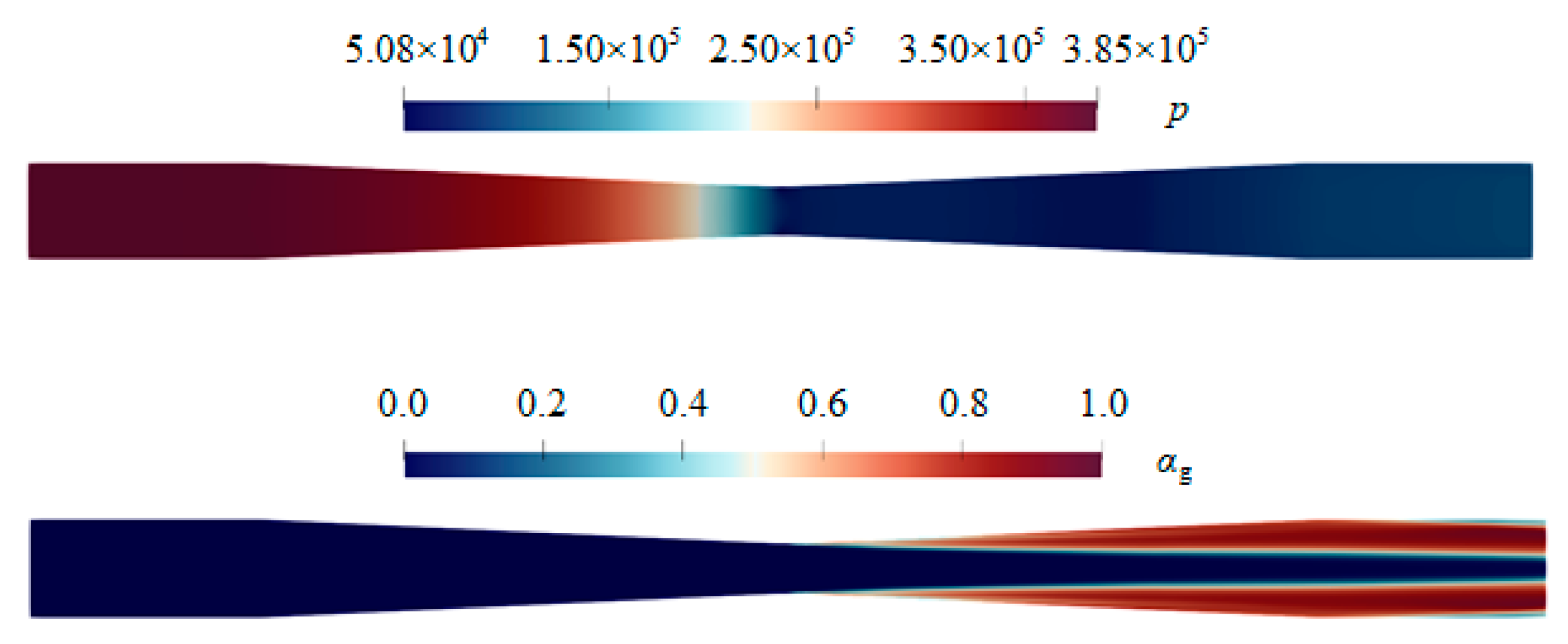
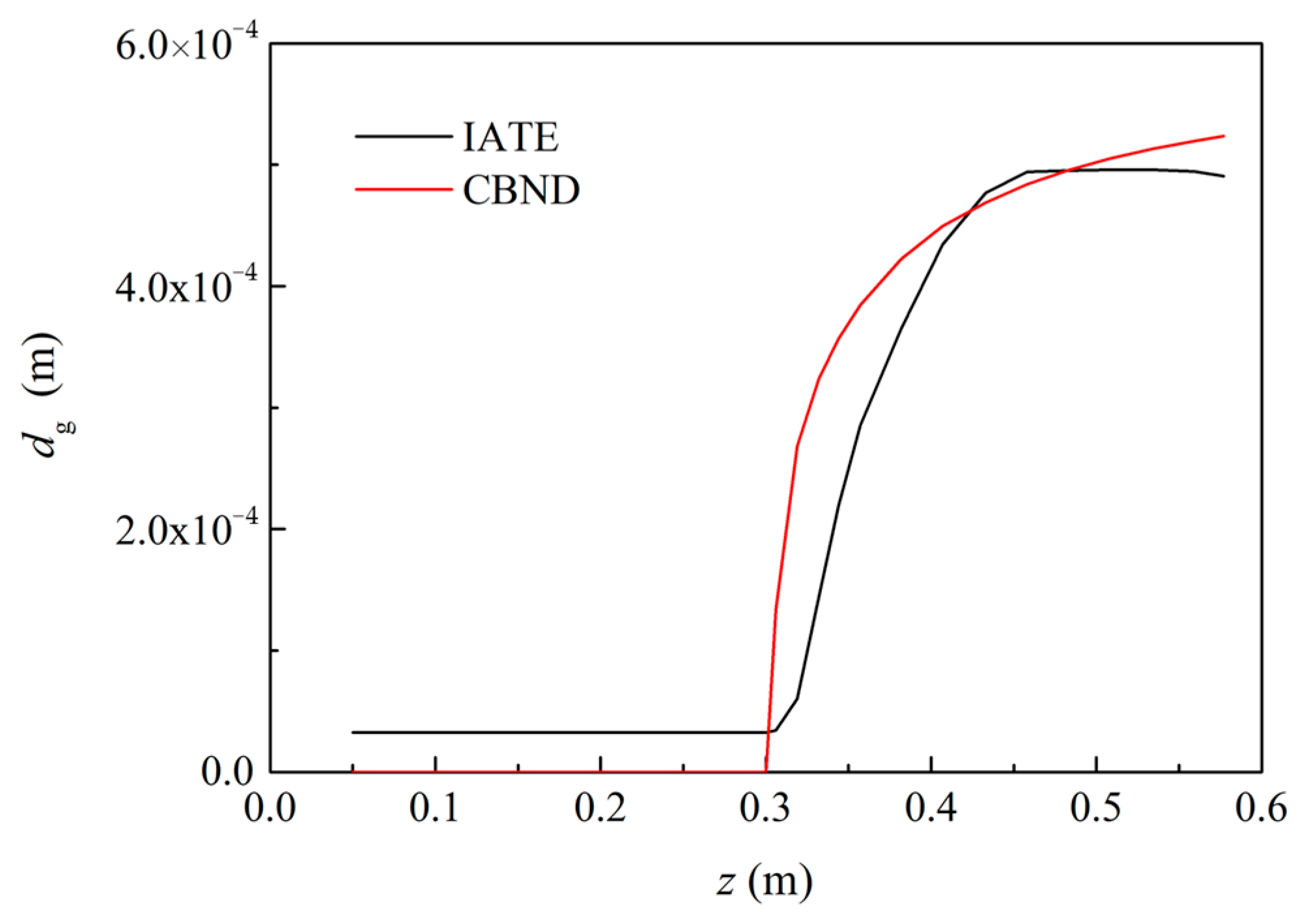
3.2. Axial Distribution of Physical Fields

As the nozzle flashing flow reaches a steady state, typical distributions of pressure and void fraction are depicted in Figure 2. The simulated axial pressure and gas volume fraction with IATE and CBND models and experimental values are shown in Figure 3 and Figure 4.

The inlet liquid temperatures of BNL358 (Figure 3a and Figure 4a) and BNL362 (Figure 3b and Figure 4b) are similar, but the latter has a higher inlet pressure and mass flow rate. It can be seen from the experimental values that BNL362 produces more steam in the diverging part. The axial pressure of the nozzle obtained by the two interfacial area concentration models is in good agreement with the experimental value. Compared with the CBND model, the IATE model calculates the flashing inception pressure (throat pressure) closer to the experimental value. It can be inferred that the bubble diameter obtained by the CBND model at the throat is larger than that of the IATE model, and the larger the bubble diameter, the smaller the gas–liquid interfacial area concentration, resulting in a decrease in the amount of steam produced; thus, the simulated value of throat pressure is correspondingly reduced. In the nozzle diverging section, the two interfacial area concentration models predict the gas volume fraction of BNL362 well but overestimate the gas content of BNL358. From Table 3, it can be seen that except for the inlet pressure, the other conditions of the two experiments are similar, but the simulated gas volume fractions of the two experiments are very close. Therefore, it can be concluded that the inlet pressure and the pressure drop in the converging section have a significant influence on flashing.

Compared with the previous two groups of experiments, the inlet temperatures of BNL291 (Figure 3c and Figure 4c) and BNL284 (Figure 3d and Figure 4d) increase, and the inlet mass flow rates increase accordingly. Both interfacial area concentration models accurately predict the flash inception pressure and the pressure variation of BNL291 but underestimate that of BNL284. As the gas reaches the outlet, the volume fraction in both experiments decreases, which can be attributed to the pressure recovery after the nozzle diverging section. Both models accurately predict this change. However, the CBND model overestimates the gas volume fraction compared to the experimental values for BNL291 and BNL284, suggesting that the model predicted a smaller bubble diameter and a higher interfacial area concentration.

According to Equation (14), it can be deduced that if the gas volume fraction remains constant, the bubble diameter will decrease when the bubble number density increases, and vice versa. Hence, it is assumed that in the diverging section, due to the coalescence and growth effects, the bubble diameter will increase while the bubble number density will decrease accordingly. However, the CBND model fails to simulate this process, leading to an overestimation of the gas volume fraction. The IATE model also shows an overestimation of the gas volume fraction, which could be attributed to the parameter settings in the coalescence and breakage model. The original model parameters are obtained from a liquid–gas flow without phase change, which may not be suitable for the flashing process. This could result in an excessive breakage frequency or an insufficient coalescence frequency. Furthermore, both models predict an early flashing inception, as evident from the distribution of gas volume fraction in the diverging section, leading to a lower inlet mass flow rate.

BNL304 and BNL309 are both high-temperature nozzle flashing flows, but their exit pressures differ. The IATE model more accurately predicts the pressure compared to the CBND model. However, both models underestimated the pressure of BNL304. Near the exit, the CBND model calculates a relatively lower pressure (corresponding to a lower saturation temperature), resulting in a greater superheat degree and a higher gas volume fraction than the IATE model. On the other hand, both models exhibit satisfying simulation results for the pressure and gas volume fraction of BNL309.

3.3. Radial Distribution of Physical Fields

Taking BNL362 as an example, Figure 5 compares the radial gas volume fraction with the experimental value. At the position close to the wall, the gas volume fraction calculated by the IATE model is higher than that of the CBND model, which is mainly due to the fact that the IATE model takes into account the wall nucleation, which contributes to the steam production; on the contrary, the gas volume fraction predicted by the CBND model at the nozzle center is higher, which is related to the smaller bubble diameter calculated by the model. Figure 6 shows the axial bubble diameter distribution obtained by the two models. It can be seen that due to the neglect of nucleation, coalescence, and other effects in the CBND model, the bubble diameter is smaller than that of the IATE model, producing a higher gas volume fraction calculated at the nozzle center. At the throat position (z = 0.3045 m), the gas is predominantly present near the wall (as shown in Figure 5a). As the height increases, the CBND model shows a wall-peak phenomenon in the gas volume fraction distribution. This is due to the change in the buoyancy force acting on the bubble, which shifts from pointing towards the wall to pointing towards the center of the pipe with an increase in bubble size. Consequently, the bubbles migrate horizontally toward the center of the nozzle.

In general, both the IATE and CBND models are mono-disperse methods, implying the existence of only one bubble diameter in a single grid cell. Both models provide good simulation results for the overall distribution of the axial and radial distributions of physical fields, with the IATE model being more accurate in predicting the starting pressure of flashing.

Figure 7 shows the radial distribution of the bubble diameter of BNL358 and BNL362 predicted by the IATE model. At the nozzle throat (z = 0.3045), the bubble diameter at the wall surface has the smallest value due to the nucleation occurring at this location. While in the center of the throat (0.00~0.01 m in Figure 8a), the bubble diameter keeps constant at its initial value of 0.001 m. This is due to the absence of nucleation or phase change in this region, resulting in an unchanged bubble diameter. At positions near the outlet (z = 0.55), the bubble diameter increases from the center toward the wall. This is mainly because most of the vapor phase is collected in the near wall region (as shown in Figure 2), resulting in a larger Sauter mean diameter. On the other hand, the bubble diameter of BNL362 is smaller than that of BNL358 at the throat, but downstream, BNL362 has a larger diameter. This may be attributed to the effects of bubble coalescence and breakup, as well as the difference in mass flow rates between the two cases.

Apart from the bubble size (or interfacial area concentration), the interfacial heat and mass transfer also relate to the superheated degree T_sup, as shown in Figure 8. At x = 0.3045, T_sup increases from the nozzle center toward the nozzle wall, primarily due to the pressure profile at this location. As shown in Figure 9a, with little change in liquid temperature, the decreasing pressure from the center to the wall leads to a corresponding decrease in saturation temperature. At x = 0.55, T_sup gradually decreases from the nozzle center to the wall. As depicted in Figure 9b, the radial pressure distribution is relatively uniform, resulting in minimal variation in radial saturation temperature. However, at locations closer to the wall, the liquid temperature significantly drops due to the absorption of latent heat during phase change, leading to the minimum T_sup in this region.

4. Conclusions

In this paper, a numerical simulation study of converging–diverging nozzle flashing was conducted. The influences of IATE and CBND models on the internal pressure, gas volume fraction, and bubble diameter distribution were compared and analyzed. Both the IATE and CBND models predicted a slightly lower inlet mass flow rate than that of the experiment. This can be attributed to the higher simulated gas volume fraction in the throat. Additionally, an inadequate pressure drop in the converging part or an early prediction of flashing inception may also result in a decrease in the inlet mass flow rate. When comparing the two models in terms of the axial physical field distribution, it was observed that both the IATE and CBND models accurately predicted the axial pressure distribution. However, the simulated vapor production in the diverging section is excessive, and the calculated axial gas volume fraction distribution deviates from the experimental data. Compared with the CBND model, the IATE model provides a more accurate prediction of the flashing inception. Based on the IATE approach, the radial distributions of physical fields are verified. The radial bubble diameter exhibits opposite distribution profiles at the nozzle throat and near the outlet, and similar results can be drawn for the superheated degree.

Although the IATE model takes into account the effects of sub-phenomena, i.e., nucleation, coalescence, and breakup on bubble diameter, the corresponding sub-models are based on cold-state experiments. Therefore, the predicted bubble diameter may be too small for phase change flows, particularly for high-temperature and high-pressure flashing flows (BNL291-BNL309). This may lead to an excessive amount of steam production in the diverging section. To improve the simulation results, a poly-disperse method (such as the PBM model) that solves the size fraction equation can enhance the accuracy of bubble size calculation as well as the void fraction and pressure distribution in the flashing process. Furthermore, closure models for those sub-phenomena need to be polished. Specifically, most of the existing bubble coalescence and breakup models are developed based on non-phase change bubbles, which inevitably bring about discrepancies when applied to growing or shrinking bubbles in flashing flows. It is recommended to conduct direct numerical simulations (DNS) or high-resolution experimental investigations to enhance and validate these models.

References

1. Li, J.; Liao, Y.; Bolotnov, I.A.; Zhou, P.; Lucas, D.; Li, Q.; Gong, L. Direct numerical simulation of heat transfer on a deformable vapor bubble rising in superheated liquid. Phys. Fluids 2023, 35, 023319. [Google Scholar] [CrossRef]
2. Lv, H.; Wang, Y.; Wu, L.; Hu, Y. Numerical simulation and optimization of the flash chamber for multi-stage flash seawater desalination. Desalination 2019, 465, 69–78. [Google Scholar] [CrossRef]
3. Sonawan, H.; Nurhidayat, D.; Saefudin, H. Influence of wall atomizer to condensation rate in flashing purification. Water Pract. Technol. 2019, 14, 872–883. [Google Scholar] [CrossRef]
4. Luo, C.; Huang, L.; Gong, Y.; Ma, W. Thermodynamic comparison of different types of geothermal power plant systems and case studies in China. Renew. Energy 2012, 48, 155–160. [Google Scholar] [CrossRef]
5. Eboli, M.; Forgione, N.; Del Nevo, A. Assessment of SIMMER-III code in predicting Water Cooled Lithium Lead Breeding Blanket “in-box-Loss of Coolant Accident”. Fusion Eng. Des. 2021, 163, 112127. [Google Scholar] [CrossRef]
6. Yu, H.; Chen, Z.; Cai, J. Accident tolerant fuel thermal hydraulic behaviors evaluation during loss of coolant accident in CPR1000. Ann. Nucl. Energy 2020, 139, 107273. [Google Scholar] [CrossRef]
7. Liao, Y.; Lucas, D. A review on numerical modelling of flashing flow with application to nuclear safety analysis. Appl. Therm. Eng. 2021, 182, 116002. [Google Scholar] [CrossRef]
8. Liao, Y.; Lucas, D. Possibilities and Limitations of CFD Simulation for Flashing Flow Scenarios in Nuclear Applications. Energies 2017, 10, 139. [Google Scholar] [CrossRef] [Green Version]
9. Al-Fulaij, H.; Cipollina, A.; Micale, G.; Ettouney, H.; Bogle, D. Eulerian-Eulerian modelling and computational fluid dynamics simulation of wire mesh demisters in MSF plants. Eng. Comput. 2014, 31, 1242–1260. [Google Scholar] [CrossRef]
10. Zhao, Y.; Peng, M.; Xu, Y.; Xia, G. Simulation investigation on flashing-induced instabilities in a natural circulation system. Ann. Nucl. Energy 2020, 144, 107561. [Google Scholar] [CrossRef]
11. Liao, Y.; Lucas, D. 3D CFD simulation of flashing flows in a converging-diverging nozzle. Nucl. Eng. Des. 2015, 292, 149–163. [Google Scholar] [CrossRef]
12. Frank, T. Simulation of Flashing and Steam Condensation in Subcooled Liquid Using ANSYS CFX. In Proceedings of the Fifth FZD & ANSYS MPF Workshop, Dresden, Germany, 25–27 April 2007; pp. 1–29. [Google Scholar]
13. Janet, J.P.; Liao, Y.; Lucas, D. Heterogeneous nucleation in CFD simulation of flashing flows in converging-diverging nozzles. Int. J. Multiph. Flow 2015, 74, 106–117. [Google Scholar] [CrossRef]
14. Hibiki, T.; Ishii, M. Active nucleation site density in boiling systems. Int. J. Heat Mass Transf. 2003, 46, 2587–2601. [Google Scholar] [CrossRef]
15. Marsh, C.A.; O’Mahony, A.P. Three-dimensional modelling of industrial flashing flows. Prog. Comput. Fluid Dyn. Int. J. 2009, 9, 393. [Google Scholar] [CrossRef]
16. Liao, Y.; Lucas, D. Numerical analysis of flashing pipe flow using a population balance approach. Int. J. Heat Fluid Flow 2019, 77, 299–313. [Google Scholar] [CrossRef]
17. Pinhasi, G.A.; Ullmann, A.; Dayan, A. MODELING OF FLASHING TWO-PHASE FLOW. Rev. Chem. Eng. 2005, 21, 133–264. [Google Scholar] [CrossRef]
18. Li, J.; Liao, Y.; Zhou, P.; Lucas, D.; Li, Q. Numerical study of flashing pipe flow using a TFM-PBM coupled method: Effect of interfacial heat transfer and bubble coalescence and breakup. Int. J. Therm. Sci. 2023, 193, 108504. [Google Scholar] [CrossRef]
19. Shin, T.S.; Jones, O.C. Nucleation and flashing in nozzles-1. A distributed nucleation model. Int. J. Multiph. Flow 1993, 19, 943–964. [Google Scholar] [CrossRef]
20. Plesset, M.S.; Zwick, S.A. The growth of vapor bubbles in superheated liquids. J. Appl. Phys. 1954, 25, 493–500. [Google Scholar] [CrossRef] [Green Version]
21. Ranz, W.E.; Marshall, R. Evaporation from drops 1. Chem. Eng. Prog. 1952, 48, 173–180. [Google Scholar]
22. Li, J.; Liao, Y.; Lucas, D.; Zhou, P. Stability analysis of discrete population balance model for bubble growth and shrinkage. Int. J. Numer. Methods Fluids 2021, 93, 3338–3363. [Google Scholar] [CrossRef]
23. Ma, T.; Santarelli, C.; Ziegenhein, T.; Lucas, D.; Fröhlich, J. Direct numerical simulation–based Reynolds-averaged closure for bubble-induced turbulence. Phys. Rev. Fluids 2017, 2, 034301. [Google Scholar] [CrossRef]
24. Liao, Y.; Krepper, E.; Lucas, D. A baseline closure concept for simulating bubbly flow with phase change: A mechanistic model for interphase heat transfer coefficient. Nucl. Eng. Des. 2019, 348, 1–13. [Google Scholar] [CrossRef]
25. Liao, Y.; Ma, T.; Krepper, E.; Lucas, D.; Fröhlich, J. Application of a novel model for bubble-induced turbulence to bubbly flows in containers and vertical pipes. Chem. Eng. Sci. 2019, 202, 55–69. [Google Scholar] [CrossRef]
26. Ishii, M.; Zuber, N. Drag coefficient and relative velocity in bubbly, droplet or particulate flows. AIChE J. 1979, 25, 843–855. [Google Scholar] [CrossRef]
27. Tomiyama, A.; Tamai, H.; Zun, I.; Hosokawa, S. Transverse migration of single bubbles in simple shear flows. Chem. Eng. Sci. 2002, 57, 1849–1858. [Google Scholar] [CrossRef]
28. Hosokawa, S.; Tomiyama, A.; Misaki, S.; Hamada, T. Lateral migration of single bubbles due to the presence of wall. Am. Soc. Mech. Eng. Fluids Eng. Div. FED 2002, 257, 855–860. [Google Scholar] [CrossRef]
29. Burns, A.D.; Frank, T.; Hamill, I.; Shi, J.M. The Favre averaged drag model for turbulent dispersion in Eulerian multi-phase flows. In Proceedings of the 5th International Conference on Multiphase Flow, Yokohama, Japan, 30 May–4 June 2004; pp. 1–17. [Google Scholar]
30. Menter, F.R. Two-equation eddy-viscosity turbulence models for engineering applications. AIAA J. 1994, 32, 1598–1605. [Google Scholar] [CrossRef] [Green Version]
31. Ishii, M.; Kim, S.; Uhle, J. Interfacial area transport equation: Model development and benchmark experiments. Int. J. Heat Mass Transf. 2002, 45, 3111–3123. [Google Scholar] [CrossRef]
32. Hibiki, T.; Ho Lee, T.; Young Lee, J.; Ishii, M. Interfacial area concentration in boiling bubbly flow systems. Chem. Eng. Sci. 2006, 61, 7979–7990. [Google Scholar] [CrossRef]
33. Hibiki, T.; Ishii, M. Development of one-group interfacial area transport equation in bubbly flow systems. Int. J. Heat Mass Transf. 2002, 45, 2351–2372. [Google Scholar] [CrossRef]
34. Ooi, Z.J.; Brooks, C.S. Two-group interfacial area transport equation coupled with void transport equation in adiabatic steam water flows. Int. J. Heat Mass Transf. 2021, 177, 121531. [Google Scholar] [CrossRef]
35. Fu, X.Y.; Ishii, M. Two-group interfacial area transport in vertical air-water flow—I. Mechanistic model. Nucl. Eng. Des. 2003, 219, 143–168. [Google Scholar] [CrossRef]
36. Blinkov, V.N.; Jones, O.C.; Nigmatulin, B.I. Nucleation and flashing in nozzles-2. Comparison with experiments using a five-equation model for vapor void development. Int. J. Multiph. Flow 1993, 19, 965–986. [Google Scholar] [CrossRef]
37. Abuaf, N.; Wu, B.J.C.; Zimmer, G.A.; Saha, P. Study of Nonequilibrium Flashing of Water in a Converging-Diverging Nozzle; Volume 1: Experimental; Brookhaven National Lab.: Upton, NY, USA, 1981. [Google Scholar]
Figure 1. Experiment of flashing flow: (a) schematic of the test section; (b) computational domain.
Processes 11 02365 g001
Figure 2. Typycial distributions of nozzle pressure and void fraction.
Processes 11 02365 g002
Figure 3. Axial distribution of nozzle pressure: (a) BNL358; (b) BNL362; (c) BNL291; (d) BNL284; (e) BNL304; (f) BNL309.
Processes 11 02365 g003
Figure 4. Axial distribution of nozzle void fraction: (a) BNL358; (b) BNL362; (c) BNL291; (d) BNL284; (e) BNL304; (f) BNL309.
Processes 11 02365 g004
Figure 5. Radial distribution of void fraction: (a) z = 0.3045 m; (b) z = 0.4 m; (c) z = 0.5 m; (d) z = 0.55 m.
Processes 11 02365 g005
Figure 6. Axial distribution of bubble diameter.
Processes 11 02365 g006
Figure 7. Radial distribution of bubble diameter: (a) z = 0.3045 m; (b) z = 0.55 m.
Processes 11 02365 g007
Figure 8. Radial distribution of superheat degree: (a) z = 0.3045 m; (b) z = 0.55 m.
Processes 11 02365 g008
Figure 9. Radial distribution of pressure: (a) z = 0.3045 m; (b) z = 0.55 m.
Processes 11 02365 g009