Article

Numerical Simulation and Experimental Study on Sediment Wear of Fixed Guide Vanes of Hydraulic Turbines in Muddy River Based on Discrete Phase Model

1
Key Laboratory of Fluid and Power Machinery, Ministry of Education, Xihua University, Chengdu 610097, China
2
Sichuan Southwest Vocational College of Civil Aviation, Chengdu 610039, China
*
Authors to whom correspondence should be addressed.
Processes 2023, 11(7), 2117; https://doi.org/10.3390/pr11072117
Submission received: 26 May 2023 / Revised: 1 July 2023 / Accepted: 12 July 2023 / Published: 15 July 2023

Abstract

:
The erosion of the fixed guide vane of a hydraulic turbine by sandy water is influenced not only by flow velocity and mud concentration but also by the direction and speed of the sandy water over the surface. This study aims to investigate the erosive effect of sediment-laden water on a specific type of hydraulic turbine’s fixed guide vane, validate the efficacy of the discrete phase model (DPM) in simulating wear on the fixed guide vane, and identify the critical areas of wear on its surface. To achieve these objectives, the wear model and DPM model are employed to conduct numerical simulations on the fixed guide vane. Additionally, samples of sand are collected from the power station site, and laboratory tests are conducted on the hydraulic turbine’s flow passage components using actual sediment concentration and sand-to-water ratio to determine the sediment wear conditions. The numerical simulation results of the guide vane’s surface wear rate are compared with the experimental data to verify the wear condition of the fixed guide vane under its rated working condition. These findings serve as a reference for the later-stage design of erosion-resistant solid guide vanes for hydraulic turbines.

1. Introduction

Many rivers worldwide contain high concentrations of sand and sediment, which inevitably leads to wear on hydraulic turbines. The damage to the turbine’s components exposed to the water flow results in decreased efficiency, frequent maintenance requirements, and unstable power supply. Consequently, the study of sand erosion in hydraulic machinery has garnered significant attention from scholars globally. This research aims to enhance the operational efficiency and stability of hydropower stations by conducting numerical simulations on a specific type of hydraulic turbine’s fixed guide vane. The simulation results are then compared with experimental data to validate the effectiveness of the discrete phase model (DPM) in simulating the wear on fixed guide vanes and to identify critical wear areas on their surfaces. Developing protective and maintenance plans against sediment erosion on fixed guide vanes is crucial for improving the operational efficiency and stability of hydroelectric power plants. Factors such as material selection, flow velocity, sediment content, and others must be taken into account.
In recent years, scholars worldwide have extensively studied various types of hydraulic machinery using DPM models. Sediment erosion on flow components of hydraulic turbines has gained widespread recognition among both domestic and international researchers through the use of numerical simulation methods. Scholarly investigations have revealed that sediment erosion on these components is primarily influenced by factors such as sediment particle size, flow velocity of sand-laden water, material selection for the flow components, and sediment content of the river in the power plant. Gongxiang Zhong focused on erosion and wear issues of a novel high-pressure manifold quick connect device used in ground-based well pads using the discrete element method (DPM) under the Eulerian–Lagrangian dual-fluid model. The study identified the erosion concentration locations of the device and factors affecting erosion size [1]. Zuobing Chen et al. examined a vertical mill and employed a combination of experimental and simulation methods. They utilized the bidirectional coupling calculation method of the DPM to determine particle motion trajectories. The study analyzed velocity, pressure, and discrete phase distribution to investigate the interaction of two-phase flow, particle classification, and screening characteristics in the vertical mill flow field [2]. Jiao Liao et al. conducted a comprehensive channel numerical simulation of a Francis turbine to analyze sediment distribution and solid–liquid two-phase velocities on the runner blade surface under different operating conditions. The study provided a theoretical basis for the hydraulic turbine’s transformation in the power station [3]. Lei Xu proposed a discrete unit method based on the Euler–Raglansi dual-fluid model capable of calculating wear caused by discrete phases of varying particle sizes [4]. Hongbin Liu employed the Fluent software DPM model to establish an erosion model for a three-way tube, obtaining erosion characteristics [5]. Jingting Zhao and Jinxi Zhu investigated the flow behavior of solid–liquid two-phase flow in pumps, specifically examining the influence of blade inlet angle, particle diameter, density variation, and pump impeller auxiliary blades on particle motion trajectories and pump performance [6]. Rennian Li and Yan Liu utilized two-phase flow theory and boundary theory to formulate a mathematical model for the boundary between a constant solid and fluid in two-phase flow [7]. Yan Cao, et al. investigated the characteristics of water-conducting components in hydraulic turbines under the influence of sandy water flow using an experimental model setup. They identified the correlation between the relative positioning of fixed and movable guide vanes and the sand content [8]. Xiaobing Liu and Liangjun Cheng, starting from the fundamental principles of fluid mechanics, analyzed the forces acting on solid particles within any flow field. They derived the motion equation for sparse solid particles, developed a numerical calculation method to solve particle motion, and established a solid–liquid two-phase turbulence model, a particle wear model, and an Eulerian–Lagrangian mixed turbulence model for water turbomachinery. Furthermore, they conducted numerical simulations to investigate sediment wear in hydraulic turbine machinery [9].
Sheldon and Finnie conducted experiments and analysis, demonstrating that certain size and flow velocity ranges of impact particles can cause plastic deformation and exhibition of wear characteristics typically observed in flexible materials [10]. Hashemisohi et al. employed a dense discrete phase model coupled with granular fluid dynamic theory and experiments to investigate the bubble characteristics and separation of multi-component particle mixtures in a fluidized bed [11]. Jafari et al. examined the erosion wear characteristics of four different wear-resistant steel plates and developed a device to evaluate erosion wear rates of various materials under different slurry concentrations [12]. Singh utilized water and ash as the continuous and discrete phases, respectively, in a solid–fluid two-phase system. The study explored the corrosion and erosion characteristics of bent pipes by analyzing factors such as speed, concentration, and particle size [13]. Sato conducted experiments using impact jet devices in air and water, as well as rotating disk devices, to analyze different modes of material failure by examining surface wear under varying particle sizes, impact angles, and flow velocities [14]. Padhy et al. performed experiments on small-scale bucket-type turbines and found that wear rates increase with sediment concentration when the impact of sand particle size is neglected. However, at constant sediment concentration, wear rates are directly proportional to sand particle size [15]. Kenichi et al. utilized a jet erosion test apparatus to evaluate wear in different materials and coatings. Results indicated that variations in impact angle between 60° and 90° have a minimal effect on wear at higher velocities (e.g., 40 m/s), while at lower velocities (e.g., 10 m/s), wear decreases with increasing impact angle up to a certain value [16]. Neppane [17], using a test apparatus developed by Thapa [18], investigated flow characteristics at the exit of axial flow turbine guide vanes and the inlet of the runner in a sand–water mixture. Findings revealed that particle trajectories deviating from streamlines during flow significantly impact wear. Moreover, larger particle sizes and higher concentrations lead to greater deviation from streamlines. Laouari et al. conducted research on steady and unsteady cavitation flow in a small-scale mixed-flow turbine using a two-phase mixture model. The researchers assessed the impact of a reduced cavitation number on hydraulic performance and determined the operating range for cavitation-free operation [19]. Yonezawa et al. conducted numerical simulations to investigate the flow of solid particles and their erosion effects within labyrinth seals. The study observed that while increased leakage flow rates significantly disturb Taylor vortices, stable vortices still form within the central space regardless of the leakage flow rate [20]. Noon et al. surveyed various techniques employed by researchers to mitigate slurry erosion and cavitation. They performed an economic analysis for a case study involving centrifugal pump (CP) usage in Pakistan, which demonstrated that an 8% improvement in pump efficiency can reduce the life cycle cost by approximately 17.6% [21]. Dahlhaug et al. investigated the performance of a Francis turbine, specifically focusing on erosion-induced clearance gaps in the guide vanes (GVs). Numerical simulations using the GV and runner blade passages revealed that the clearance gap induces a leakage flow due to pressure differences between adjacent sides. This leakage flow mixes with the main flow, creating a vortex filament inside the runner. The asymmetrical profiles examined in the study exhibited improved erosion resistance, efficiency, and pressure pulsations in the runner. By incorporating non-uniform clearance gaps in the analyses, the influence of leakage flow on the runner can be more accurately studied [22]. Thapa et al. investigated the impact of clearance gaps in GVs of Francis turbines, which contribute to total losses due to the formation of secondary flow within the gaps. The study concluded that clearance gaps of up to 0.5 mm (at 97 mm GV height) can be tolerated without causing significant losses in low specific speed turbines [23].
Various experimental methods have been employed to study sediment erosion in hydro turbines, including jet impact, rotating container, vibration impact, rotating test specimen, sediment swirling, and local bypass methods. However, the accuracy of wear tests is often compromised by the limitations of current experimental devices and methods. It is crucial to simulate the actual flow conditions of hydro turbine components as closely as possible. Among the readily available experimental methods, the rotating wear test involves machining turbine components into various shapes, fixing them on a rotating disc, and examining the wear behavior of different materials at different rotational speeds. While this method is conceptually simple, it only provides information about the relationship between water flow velocity and material wear, lacking flow similarity. As a result, it cannot accurately estimate the extent and distribution of wear on hydro turbine components.
To address these limitations, this study introduces an innovative flow-around test method. The principle involves numerically simulating the complete flow field of a hydro turbine under different operating conditions to determine the flow distribution around the critical overcurrent component, specifically the fixed guide vane. This information serves as the foundation for designing a test apparatus that replicates the flow passage of the overcurrent component, enabling wear tests. This approach ensures flow similarity between the test specimen and the actual turbine, resulting in consistent results with real-world performance. It facilitates convenient analysis of wear patterns on the test specimen and offers improved precision compared with other wear prediction methods, ensuring alignment between the test results and actual outcomes. This innovative approach is a notable contribution of this research.

2. Mathematical Model

The Eulerian multi-phase flow model is capable of simulating the flow and interaction between multiple phases. In this model, each phase can represent a combination of gas, liquid, and solid, and the Eulerian method is applied to each phase. Theoretically, the Eulerian model can simulate any second phase as long as there is sufficient memory capacity. However, when dealing with more complex multi-phase flow problems, the convergence of the solution results can be limited.
In the Eulerian–Lagrangian dual-fluid model, particles are treated as discrete phases, coexisting as a continuous medium. This study utilizes the K-ε model to simulate the turbulent flow of the liquid phase. It assumes that the inner flow field consists of only a clear water phase (continuous phase) and sediment phase (discrete phase), with stable physical properties for both phases. The granular dynamics method is employed to simulate the flow of the discrete phase particles, while numerical analysis is used to study the flow characteristics of a specific type of hydraulic turbine when the fixed guide vane is in operation. In the calculation of the two-phase flow, the water phase is first solved under the Euler coordinate system, which involves solving the control equations for the continuous phase. Once the calculation converges, the discrete phase particles are injected into the flow field, and then the discrete phase is solved under the Lagrangian coordinate system to obtain the flow characteristics of the discrete phase particles.

2.1. Continuous Phase Control Equation

Since there is no mass transfer between phases, the conservation equation for continuous phase quality and the dynamic equilibrium equation can be described as follows:
α c ρ c t + α c ρ c U C = 0
α c ρ c U c t + α c ρ c ( U C U C α c ρ c R C = α c p + α c ρ c g A 1
where α c is the phase fraction of the continuous phase; ρ c is the density of the continuous phase; U c is the average velocity of the continuous phase; R c denotes the stress tensor; p is the average pressure; g is the gravitational acceleration vector; and A is the momentum interface exchange term.

2.2. Discrete Phase Control Equation

In the movement of the flow field, discrete phases primarily experience drag, gravity, buoyancy, and collision forces among themselves. Due to the significant differences in magnitude between gravity, buoyancy, and collision forces within the solid phase of the liquid phase, this research primarily focuses on the drag force, while neglecting the other forces. Since the discrete phase model does not take into account collisions between discrete phases or the volume of the discrete phase itself, the movement of the discrete phase can be described as follows:
m p i d u p , x i d t = F D r a g , x i + m p i g x ρ p ρ g ρ p m p i d u p , y i d t = F D r a g , y i + m p i g y ρ p ρ g ρ p m p i d u p , z i d t = F D r a g , z i + m p i g z ρ p ρ g ρ p
where m p i is the mass of the discrete phase; u p , x i , u p , y i , u p , z i is the discrete velocity component along the x, y, and z directions; F D r a g , x i ,   F D r a g , y i ,   F D r a g , z i is the component of the drag force in the discrete phase in the x, y, and z directions; ρ is the discrete phase mass density; and gx, gy, and gz are the components of gravitational acceleration in the x, y, and z directions, respectively.

2.3. Wear Model

The general wear model used in the DPM model is as follows [24,25]:
R e r o s i o n = P = 1 N p a r t i c l e s m b C d p f α v b v A f a c e
where C(dp) is a discrete phase diameter function; α is the impact angle between the discrete phase and the wall surface; ν is the discrete phase velocity; b ( ν ) is a function of relative velocity; and I is a function of impact angle.
f α = sin ( 2 α ) 3 sin 2 α ,   tan α 1 3 1 3 cos 2 α ,   tan α > 1 3

3. Numerical Simulation Analysis of Sediment Erosion of Fixed Guide Vanes of Hydraulic Turbines

With the advancement of computational fluid dynamics (CFD), numerical simulation has emerged as a crucial tool for studying fluid dynamics. Extensive research on CFD methods and the development of corresponding software have led to significant improvements in accuracy, reliability, and computational visualization. By conducting numerical analysis and calculations of three-dimensional flow fields, it is possible to predict the performance of hydraulic turbines and validate the reliability of substituting model tests with numerical tests for flow passage components. In this study, a three-dimensional geometric model of the fixed guide vane for the flow passage component is created using three-dimensional modeling software, such as UG, based on the design drawings. Calculation conditions are determined considering the actual operating conditions of the hydropower station, while also considering the coupling relationship between various flow passage components. CFD software is then employed to analyze and calculate the three-dimensional viscous flow of sandy water throughout the entire flow passage. This enables the analysis of flow conditions in different flow passage components under various operating conditions, providing a robust reference for the operation of power station units.

3.1. Three-Dimensional Model and Grid Division of Fixed Guide Vanes of Hydraulic Turbines

Geometric modeling of the hydraulic turbine is conducted, as depicted in Figure 1. The excessive pathways of the hydraulic turbine are divided into four sections. Figure 1a presents an overall three-dimensional model diagram of the hydraulic turbine, while Figure 1b illustrates an exploded view of the hydraulic turbine in three dimensions.
This study focuses on the investigation of a specific type of hydraulic turbine’s fixed guide vane. The design of the fixed guide vane serves as the basis for creating B-spline curves (NURBS) for the front and back surfaces of the guide vane using UG software. Subsequently, the tail sidelines and head arcs are constructed. These four curves are then enclosed in the XY plane to form an airfoil shape. The relevant data of the fixed guide vane are imported into UG software, and the three-dimensional modeling function is utilized to generate a solid representation of the guide vane, as depicted in Figure 2. Following this, grid generation is conducted using ICEM software. The resulting grid for the guide vane’s flow passage calculation is presented in Figure 3, the enlarged view of the red area is shown in Figure 4.
Based on the design parameters and operational range of the hydraulic turbine, specific operating points are selected from the comprehensive curve of the model for full flow field simulation analysis. A single flow path is extracted, and the blade length is reduced to 0.2 in accordance with the similarity principle. The original streamline is designed as the wall surface of the hydraulic turbine’s fixed guide vane, and the guide vane is positioned accordingly (Figure 5). The geometric conditions, physical conditions, boundary conditions, and initial conditions of the flow field are all based on the similarity principle, enabling an approximate simulation of the flow field surrounding the fixed guide vane of the hydraulic turbine.
For this study, the dedicated CFD preprocessor ICEM software is employed to create an unstructured grid for the flow passage components, with mesh size based on the reference [26]. The first layer grid height is set at 0.01 mm, and local grid refinement is applied at the leading and trailing edges of the blade. The outlet flow rate is selected as the reference standard for assessing grid independence. After validation, the final confirmed grid number is 3305421 (Figure 6).
The grid size in the simulation should be larger than the size of sediment particles, ideally around 1.25–1.5 times the sediment size, to obtain the most reasonable results. In this study, three cases were considered for Δ/db ratios: 1, 1.25, and 2. Among these, when the grid size is approximately 0.0875 mm (corresponding to Δ/db = 1.25), the velocity distribution curves of the liquid and solid phases best match the experimental data, while other grid sizes show varying degrees of deviation (Table 1). When the Δ/db ratio is 1 or 2, the overall flow velocity significantly exceeds the experimental values. This discrepancy is caused by numerical dispersion due to small grid ratios and overestimation of vortex scale division limits in solid–liquid two-phase flow for large grid ratios. The grid size plays a significant role in the velocity distribution within the core region and near the wall. Based on the previous analysis, the impact of the boundary layer on circular pipe simulation is discussed for cases using the WALE model and a mainstream grid size of 0.0875 mm. It is observed that densifying the wall grid in the normal direction leads to a closer match between the distribution of liquid phase velocity and experimental results, as well as a more uniform energy distribution along the pipe diameter. Different levels of densification may cause slight variations in velocity. A thinner boundary layer yields better simulation results while saving computational resources. Comparison with the simulation results without boundary layer densification reveals that the non-densified results exhibit approximately 8% higher liquid phase velocity and more pronounced variations near the wall. Hence, a 2% densification for the boundary layer is selected as the final simulation setting.
The discrete phase module of commercial CFD software is utilized to simulate the flow field, with the following key settings: Firstly, the standard K-ε turbulence model is selected, and the inlet boundary condition is set as a velocity inlet with a velocity of 6.53 m/s. It is assumed that the velocity of the discrete phase is equal to that of the continuous phase. The discrete phase enters the flow field through the inlet surface with a mass flow rate of 2.11 kg/s. The outlet boundary condition is a pressure outlet set at 101,325 Pa, which corresponds to standard atmospheric pressure. The discrete phase is completely expelled at the outlet. The turbulence intensity is set at 5%, the particle size at 0.0001 m, and the wall surface conditions are specified as a non-slip rough wall surface with a roughness of 1 × 10⁻⁴. The wall surface recovery coefficient is set at 0.98, indicating that there is 2% loss of momentum after the collision between sediment particles and the wall surface of the movable guide vane, and that the particles and wall surfaces are fully flexible. The standard wall function is employed for the near-wall surface, considering accuracy. The impact angle function is constant at 2.6. Since the DPM does not account for the volume fraction and the relative continuous phase of the discrete phase, the volume fraction of the discrete phase should not exceed 10%.

3.2. Numerical Simulation Calculation Results of Sediment Wear on Fixed Guide Vanes

Figure 7, Figure 8, Figure 9 and Figure 10 illustrate the pressure distribution and sediment volume fraction distribution of the guide vanes under design conditions. The pressure distribution diagram demonstrates a well-balanced and smooth transition with good symmetry in the circumferential direction. The sediment volume concentration distribution diagram reveals that the lower surface of the water guide mechanism exhibits relatively high sediment content due to the gravitational effect on sediment particles. Furthermore, the impact of sediment particles on the guide vane head leads to a backflow phenomenon, resulting in a higher sediment concentration at the head.
Consistent with the high flow region on the fixed guide vane wall surface, Figure 11, Figure 12 and Figure 13 reveal a consistent trend in pressure variation. Along the chord direction of the airfoil, the pressure on the working surface of the fixed guide vane gradually decreases, while the pressure on the back side of the fixed guide vane head initially stabilizes and then increases. The impact of the water flow on the fixed guide vane head leads to backflow and secondary flow phenomena, causing a significant pressure drop on the back side of the fixed guide vane head.
Figure 14 illustrates the wear rate distribution on the working surface and back surface of the fixed guide vane of the hydraulic turbine. Figure 15 presents the variations in sediment concentration and flow velocity along the height of the fixed guide vane at the 1/2 position. In this study, the particle concentration at each position is primarily influenced by the impact angle, flow velocity, and blade geometry. Considering the sidewall effect, this research focuses on the fully developed turbulent region, specifically the changes in the fixed guide vane at the 1/2 height position. The results depicted in Figure 15 show that, despite a relatively higher string length (0.6 to 0.9), the sediment concentration remains low, yet the wear rate is still significant. This can be attributed to the impact angle and power in this specific region. Due to inertia, sand particles penetrate the high-pressure zone of the boundary layer and collide with the wall surface. Although there are variations in sediment concentration at different blade positions, the changes along the same string are not substantial. Therefore, it is inferred that the impact angle and flow velocity along the same string have the most significant influence on the wear rate.

4. Experimental Study on Sediment Wear Characteristics of Fixed Guide Vanes of Hydraulic Turbines

Sediment concentration in rivers is a common occurrence, and hydraulic turbines worldwide face challenges related to sediment wear. The main steps of the flow-around wear test are outlined as follows:
Step 1: Ensure that the sediment concentration of the test sand aligns with the actual discharge of the power station. Based on the three-dimensional numerical simulation results of a prototype hydraulic turbine, the flow conditions of a single channel within the turbine’s water guide mechanism are analyzed. The flow lines around the flow passage are extracted to define the flow boundaries, and a test piece resembling the flow passage components of the real power plant is designed, specifically for the fixed guide vanes.
Step 2: Adjust the parameters and selection criteria for the sediment, such as particle size and the actual operating conditions of the hydropower station. Fine-tune the water-to-sand ratio and flow rate in the test system accordingly. Conduct the abstinence and wear test, allowing a sufficient duration for the test to take place. Once completed, remove the test parts and utilize a white light interference contour meter to measure the surface wear depth and appearance. Utilizing the multi-linear analysis method, establish the wear equation and associated indices.
The equation for sediment wear rate can generally be expressed as follows:
E ˙ = k ϕ p W n
where E ˙ is the wear rate (the wear depth per unit time of the surface material of the flow passage component) (µm/h); k indicates the coefficient of sediment particle characteristics, material characteristics of flow passage components, and other influences; ϕp is the sediment volume fraction on the surface of the flow passage components, which are related to the sediment concentration or sediment concentration CV at the inlet of the hydraulic turbine, the geometric shape of the flow passage components of the hydraulic turbine, the operating conditions of the hydraulic turbine, etc.; W is the relative velocity of sand water or sand particles impacting the surface of the flow passage component (m/s); and n is the speed index.
Step 3: Utilize the numerical calculations to extract the velocity and concentration distribution data for crucial components of the hydraulic turbine. Subsequently, incorporate these data into the quantitative wear rate equation to make predictions regarding the wear condition of the hydraulic turbine.

4.1. Flow-Around Wear Test

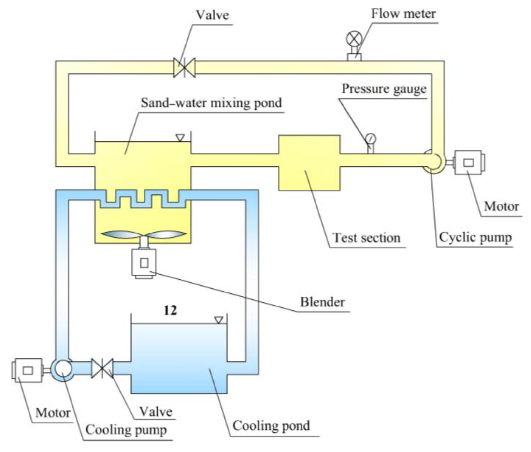
The experimental setup comprises the power system, cooling system, sediment mixed system, and test section, as depicted in Figure 16. The maximum power capacity of this experiment is 630 kW, with a sand pool volume of 30 m3. The system employs stainless steel pipes with a diameter of ϕ 200 mm and operates at a pressure of 376 m water column. The rated flow rate is 482 m
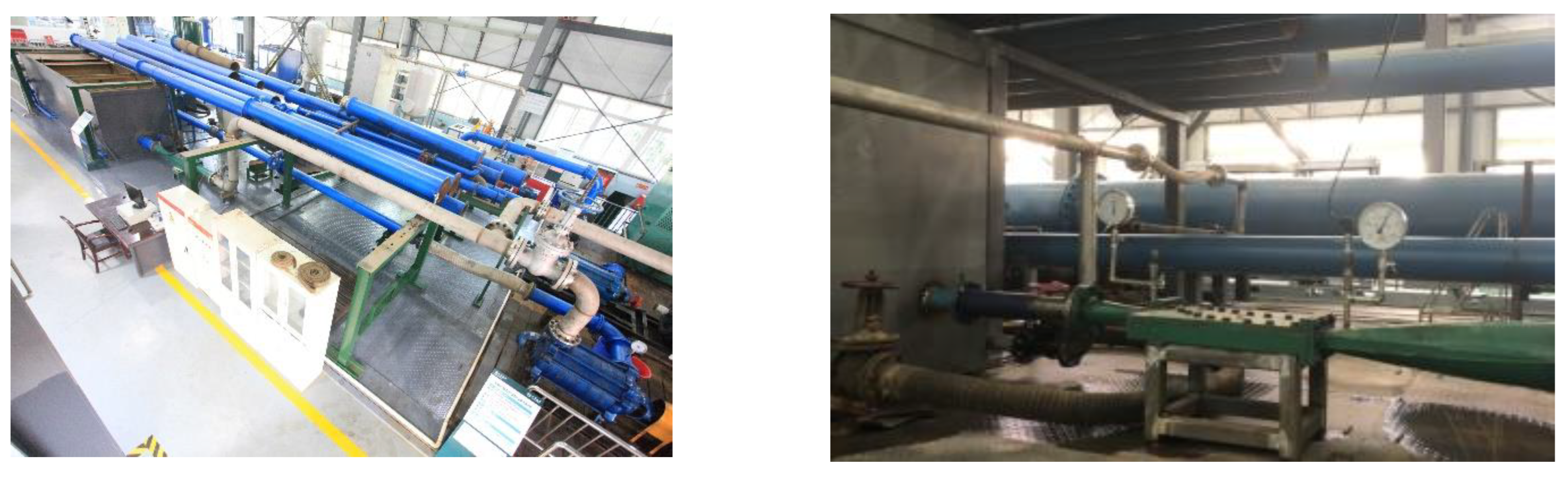
3/h. To achieve a homogeneous sediment mixture, the sediment mixed system utilizes a water pump for impact and stirring. For cooling purposes, a snake-shaped tube is employed to extract groundwater. The test site is illustrated in Figure 17.
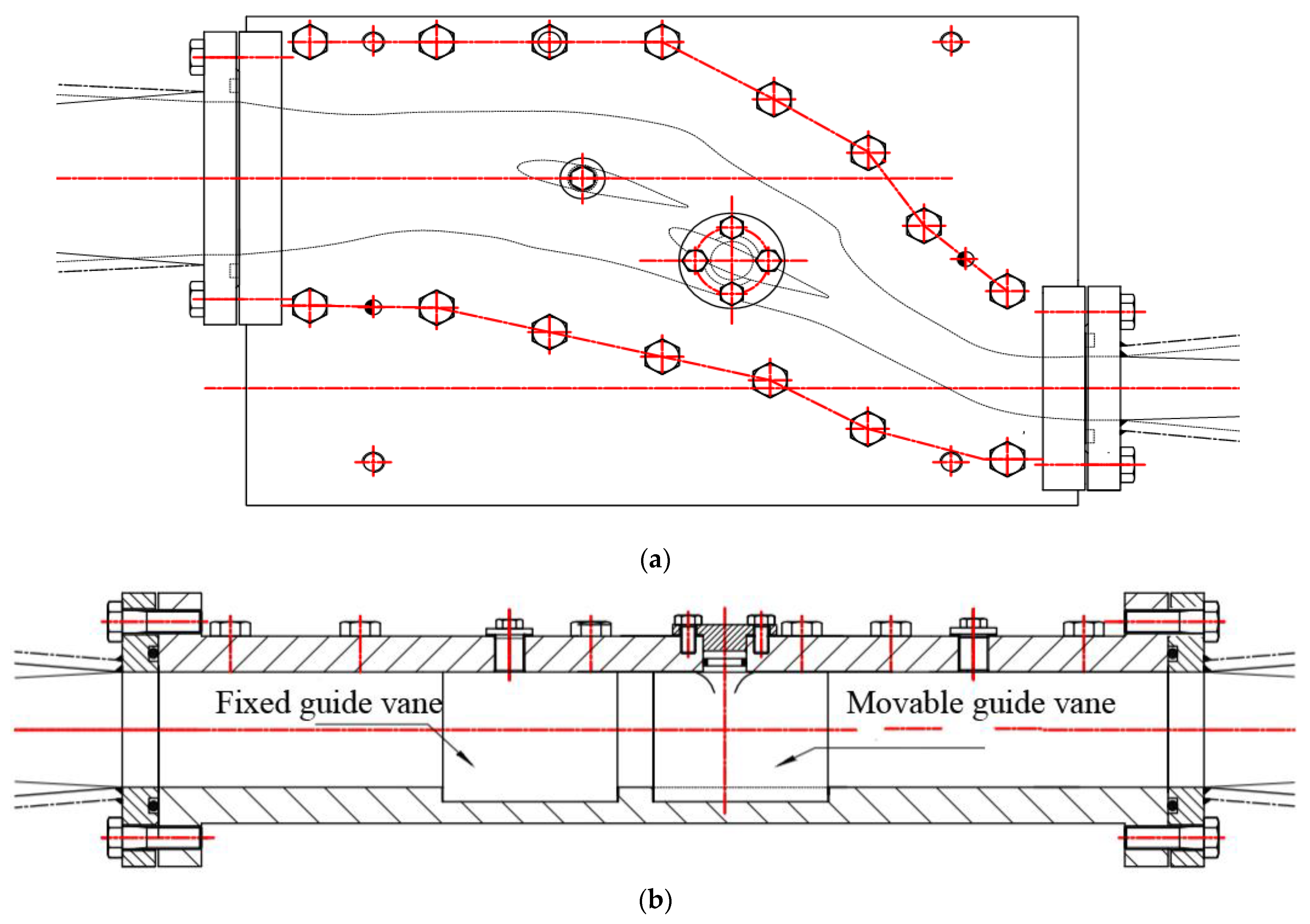
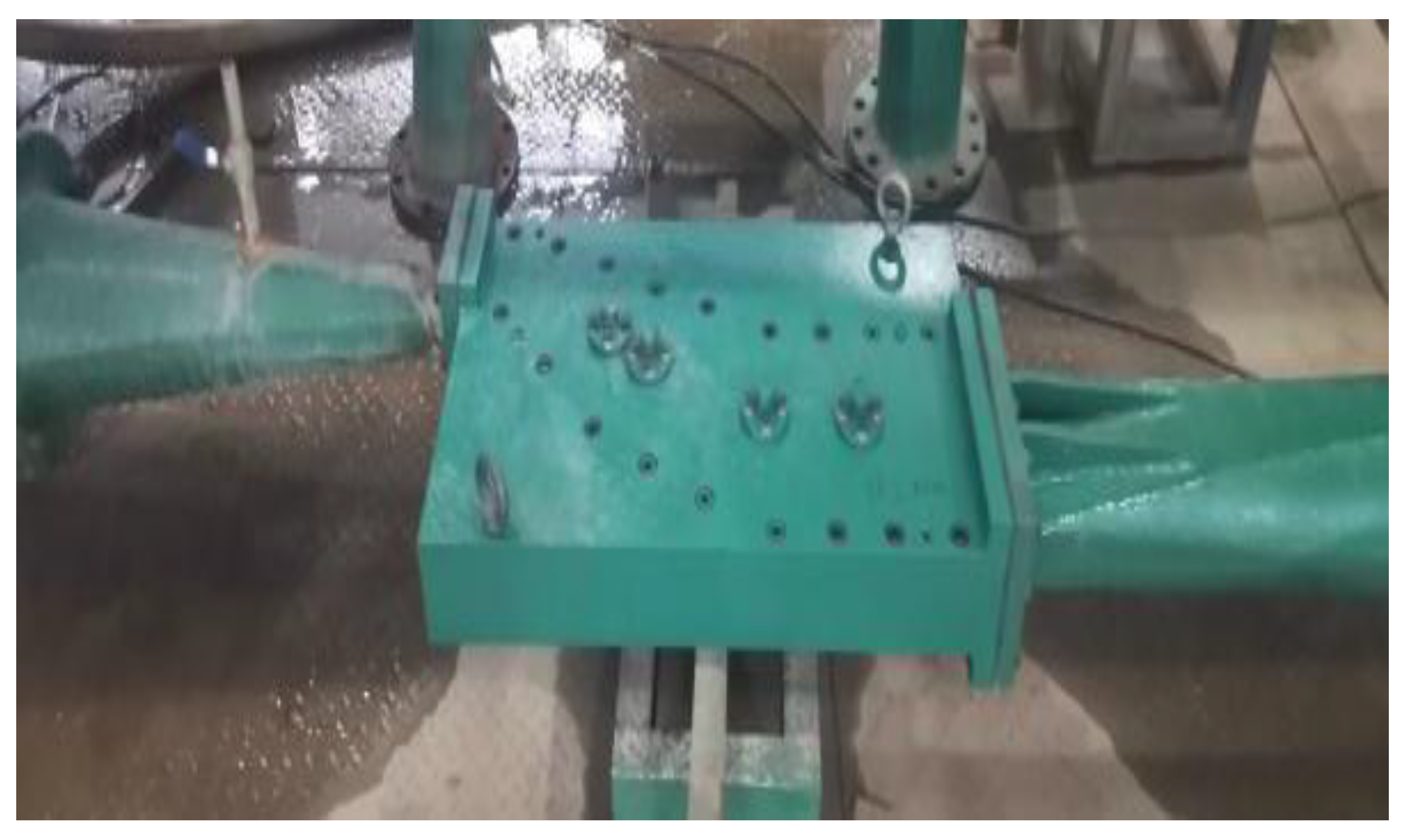
The test section plays a crucial role in the experimental setup. In the case of the fixed guide vane of a specific type of hydraulic turbine, the test section is constructed using Q345 carbon steel. To align with the flow field profile obtained from numerical simulations, the test section undergoes CNC machining to create water channels with a depth of 40 mm for the water guide mechanism under various operating conditions. At the bottom of the flow channel, a groove with a depth of 6 mm is milled to accommodate the installation of the guide vane, ensuring a snug fit between the guide vane and the groove. Figure 18 presents a sectional machining drawing of the working section, while Figure 19 shows a single passage diagram for the guide vane wear test section. Additionally, Figure 20 provides a physical photograph of the test section box, and Figure 21 displays pre- and post-installation photographs of the guide vane in the test section.
The key characteristics of sediment particles found in the power station are presented in Table 2. Additionally, Table 3 displays the particle grading of suspended sediment samples, while Table 4 provides the mineral composition analysis. The density of quartz ranges from 2.5 to 2.8 g/cm3, typically averaging 2.65 g/cm3. Calcite has a density of 2.60 to 2.8 g/cm3. Feldspar has a density of 2.55 to 2.57 g/cm3, and chlorite has a density of 2.65 to 2.9 g/cm3. To ensure similarity between the working conditions of the fixed guide vane for a specific type of hydraulic turbine and the experimental setup, a sand sample from the power station is utilized. The power station’s sand sample contains a maximum sand content of 9.52 kg/cm3. The fixed guide vane is made of Q345R material, and its boundary conditions align with those employed in the numerical simulation.

4.2. Numerical Treatment of Sediment Abrasion Test for Fixed Guide Vanes

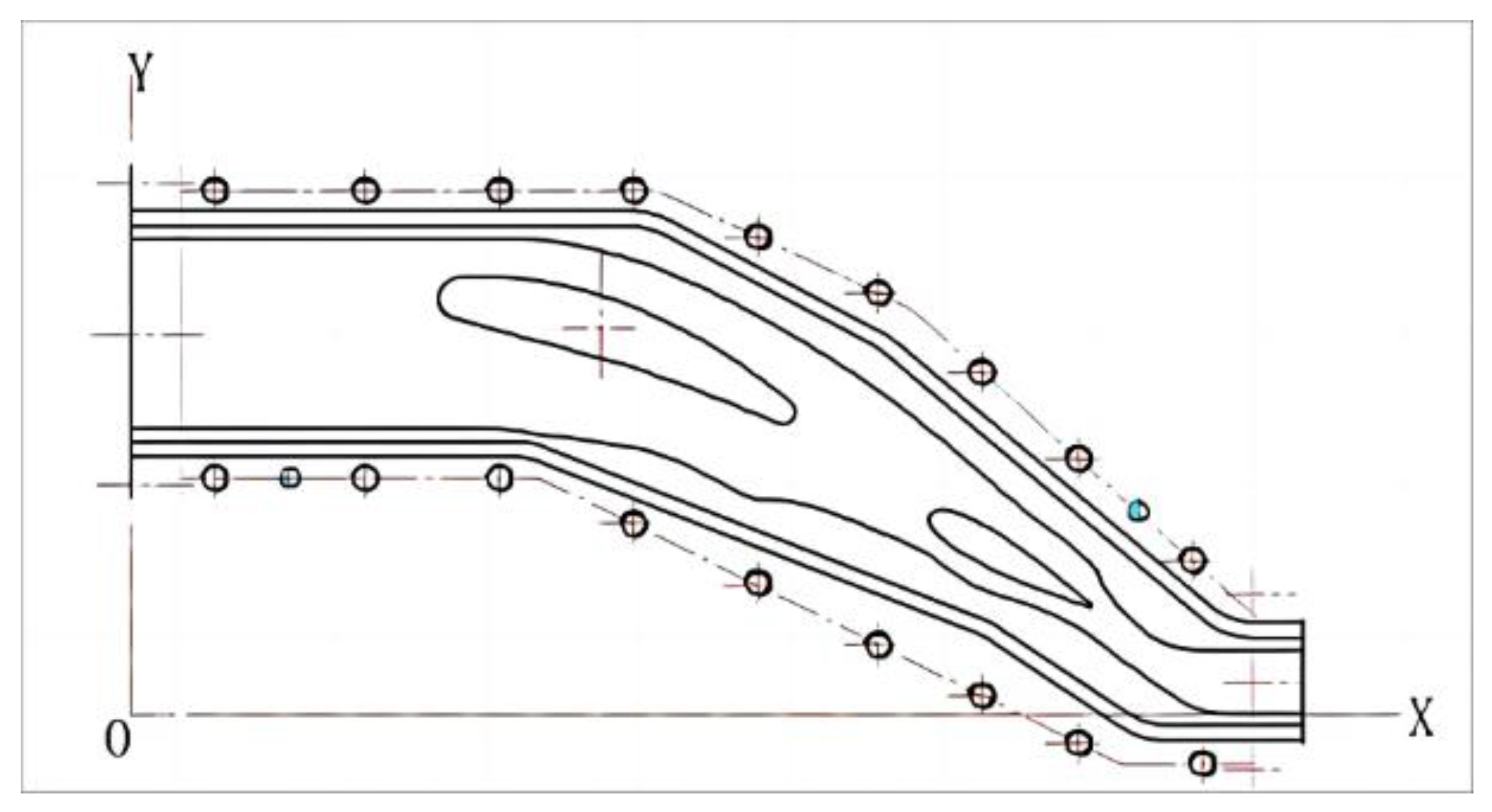
In this study, the depth test method is employed to assess the specific location wear on the surface of the test specimens in order to quantify sediment wear. Prior to conducting the tests, the surface measurements of the vanes are marked at specific positions, ensuring that the same locations are measured before and after the test to accurately assess wear. The positions of the test specimens are determined based on the coordinates shown in Figure 22: The x-axis represents the string line direction in the side view of the vane, the y-axis indicates the height direction at the edge of the vane, and the z-axis represents the surface height of the guide vane.
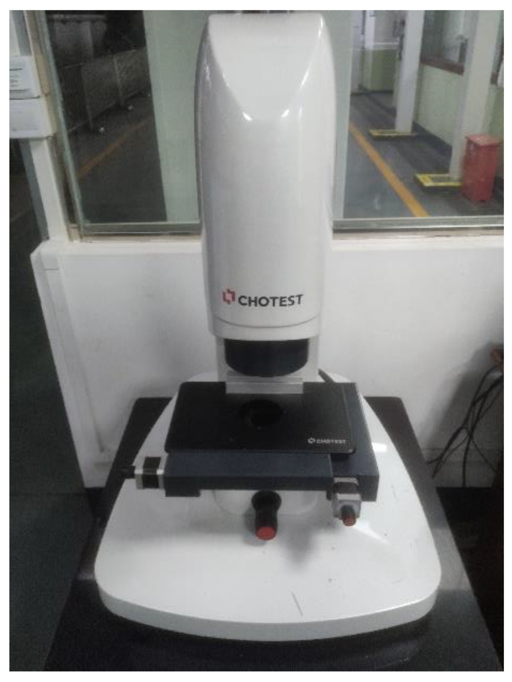
The instrument used to measure the wear depth and surface morphology of the test specimens is an advanced white light interference profiler (Figure 23). This instrument operates based on the principle of comparing the deviation of the test surface from an ideal reference surface using interference fringes. It is a high-speed, non-contact wear testing device with a measurement accuracy of 0.1 nm.
The test component is aligned with the reference point, and the position of the probe and testing stage is calibrated using the corresponding control software on the computer. Subsequently, data are collected and processed using the image acquisition system to determine the wear depth on the surface of the guide vane. The surface profiles before and after wear are measured using a white light interferometer. The wear at each position is calculated as the average difference between the working surface and the back surface at the corresponding chord length position. Figure 24 illustrates the process, where the heights of the surface at the testing positions before and after wear, denoted as z1 and z2, respectively, are measured using a white light interferometer. The difference between z1 and z2 represents the wear depth of the surface.
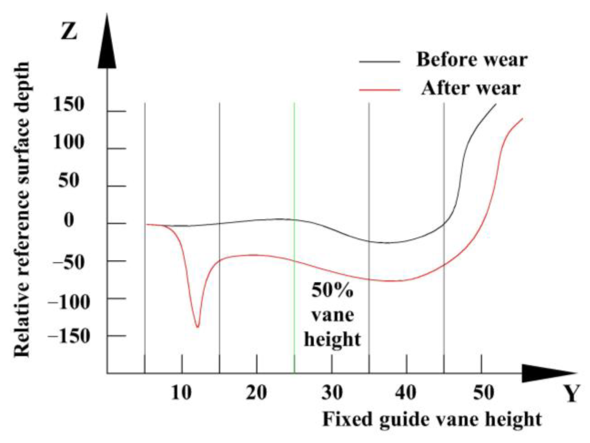
Although sediment wear serves as the fundamental design criterion, the test box introduces slight variations compared with the multi-vane flow in the actual machine. Additionally, the presence of gravity affects the test part near the upper and lower end surfaces due to sedimentation. To obtain more accurate wear depth data and mitigate these influences, the surface measurements near the 1/2 guide vane height are considered as the test results in this study.
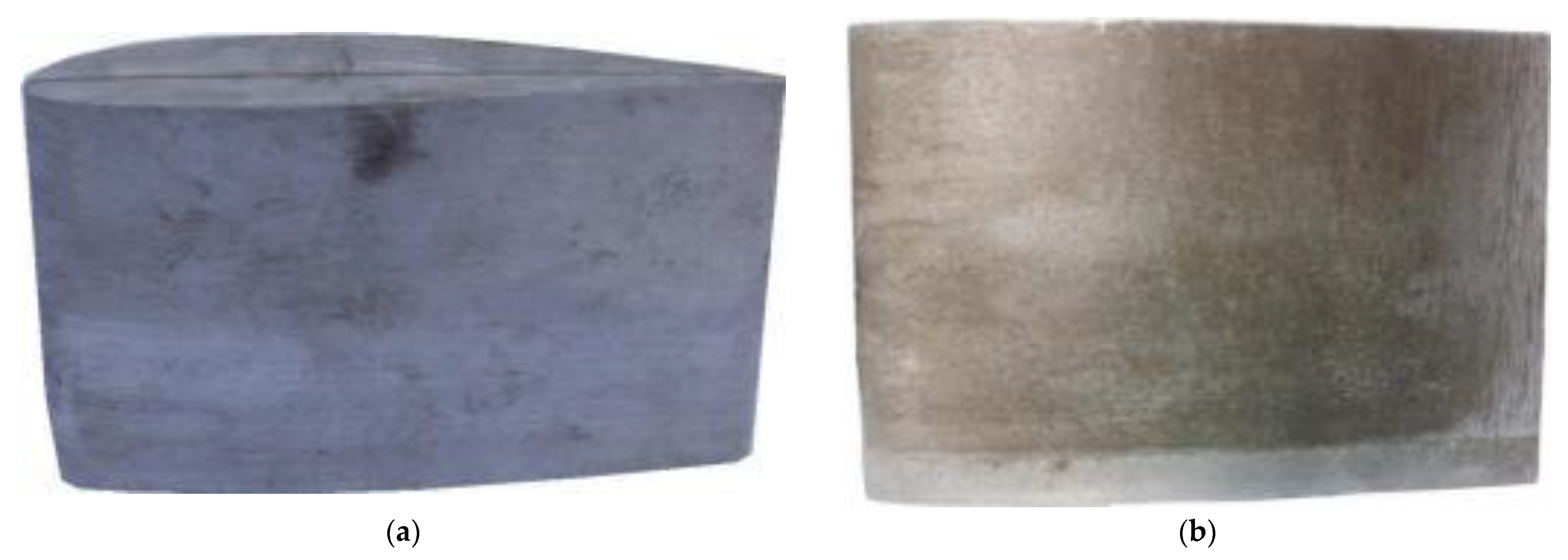
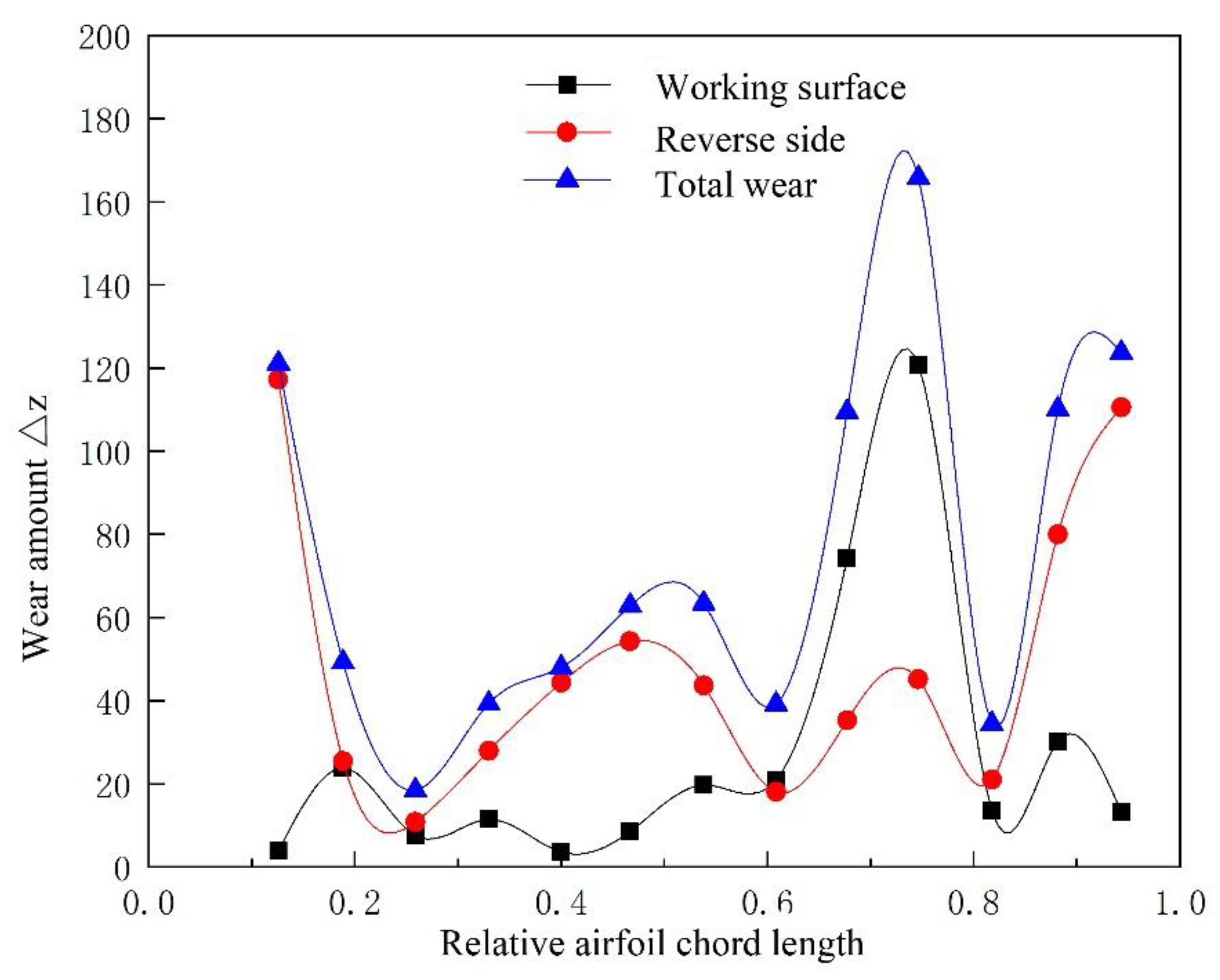
After conducting a 48 h fixed guide vane wear test, the front wear and rear wear are depicted in Figure 25. The average values within the 40% to 60% range of the blade height at the working surface and back are taken. To minimize the impact of sidewall effects, it is advisable to select 50% of the blade height. A wear distribution map is generated using a total of 26 data points, as illustrated in 
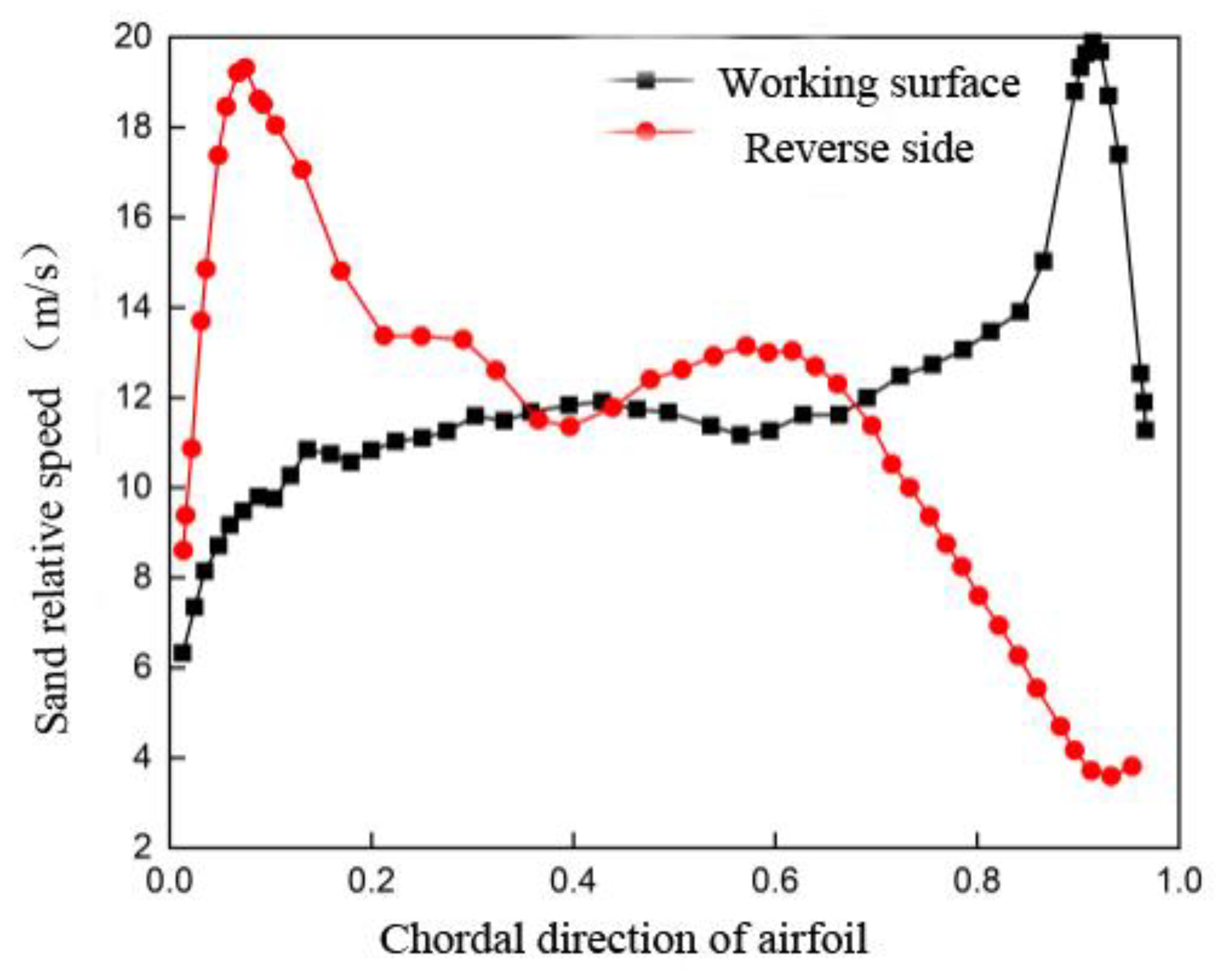
Figure 26. It is evident that the combined wear on the working surface and back of the movable guide vane exceeds 40 µm, with a maximum total wear of approximately 170 µm occurring at around 0.7 (near the tail) relative to the wing strings. Furthermore, the working surface of the fixed guide vane experiences a float of approximately 20 µm, while the back exhibits mostly greater wear than the working surface due to higher circumferential speed.

4.3. The Wear Rate Quantitative Equation Is Determined

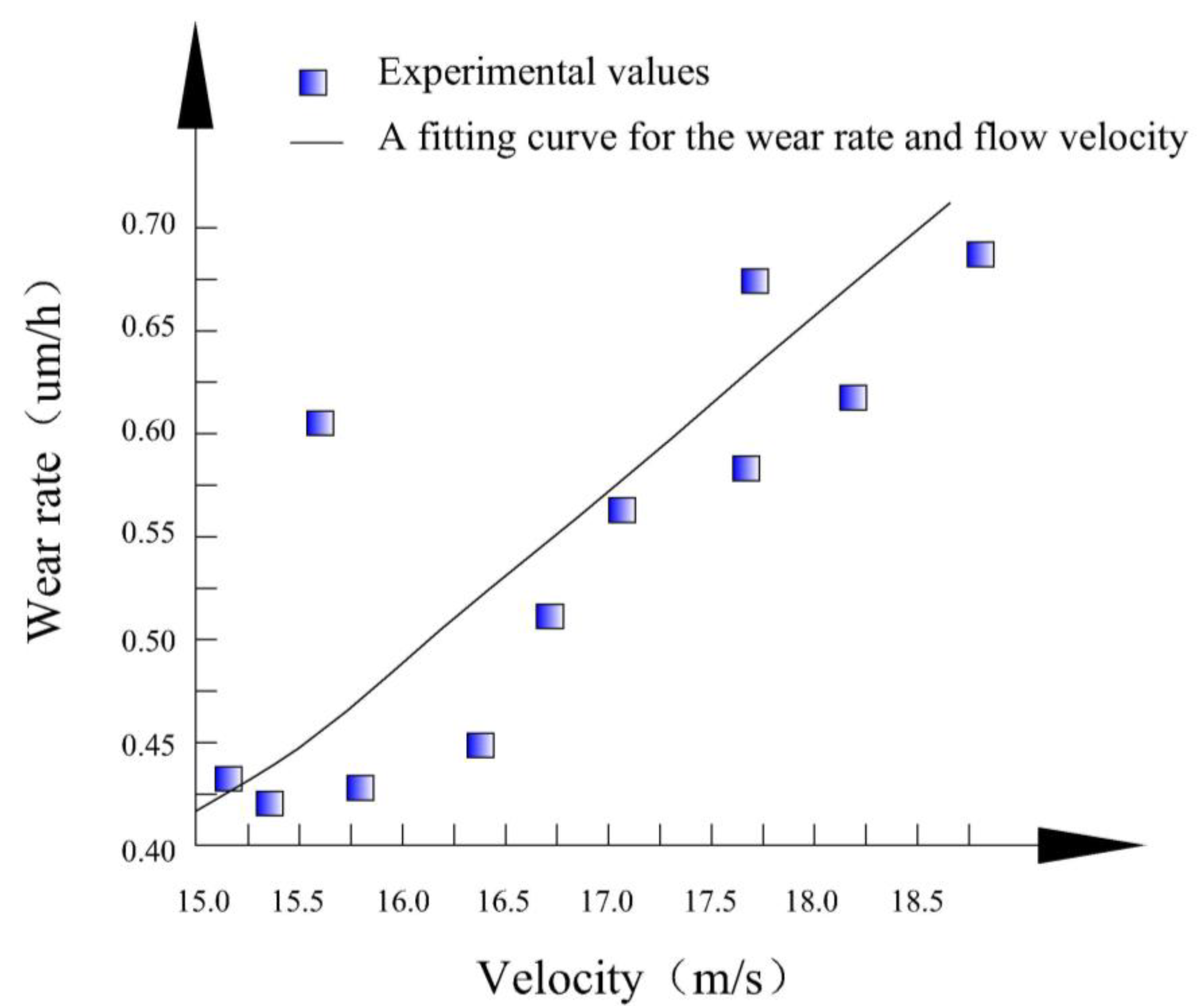
The wear rate is calculated using the equation E = KCVWn, where E represents the wear depth per unit time, given by E = (z1 − z2)/t. The relative sand flow rate (W) at the test position of the test parts is obtained from the numerical calculation results. Therefore, when sorting the data, the parameter that requires velocity is represented by index n and coefficient K.
To determine the wear rate E (µm/h), the wear amount is divided by the test duration. The velocity and wear rate of each test location are then fitted in Origin using a non-linear fitting method, specifically the Allometric function type, and the iterative algorithm for orthogonal distance regression (Pro). This process yields a fitting curve for the wear rate and flow velocity, as depicted in Figure 27.
The sand content (CV) is measured as 9.52 kg/m3, and based on this, the setting coefficient K and index n in the equation are calculated for the test parts, as shown in Table 5.

5. Comparative Analysis of Simulation and Experimental Results

In order to minimize the impact of the boundary layer on the wall surface of the flow passage, wear measurements were taken from the midpoint of the blade height. Figure 28 shows that the experimental data and simulated values exhibit a similar trend in wear rate. However, discrepancies can be attributed to the actual sediment composition, which consists of various hardness components. In the calculations, a single hardness component assumption is used, neglecting the different hardness components present. Moreover, the lift force, viscous drag, and BASSET force of the discrete phase are influenced by the volume equivalent diameter of the particles. In the simulation, the particles’ surfaces are assumed to be smooth, resulting in frictional wear upon collision with the wall surface. However, in reality, there are two types of wear: frictional wear and cutting wear. Hence, although the wear measurements in the experiment and simulation are similar, they are not identical due to the presence of both wear types in the actual scenario.
Figure 28 illustrates that the wear rate is significantly low in the 0.3–0.5 position. This is because, at this position, the discrete phase experiences a strong drag force, resulting in a low radial velocity and minimal impact from inertial forces. Overcoming the secondary flow and resistance within the high-pressure region of the boundary layer becomes challenging, resulting in a decrease in kinetic energy when the discrete phase collides with the wall and consequently a lower wear rate. As the chord length increases, the impact angle and wall surface angle continuously change, leading to an increase in the impact angle and velocity, reaching its maximum at the 0.9 chord length position. This results in a higher kinetic energy for the discrete phase to overcome the secondary flow and resistance within the high-pressure region of the boundary layer. Additionally, as the impact angle changes, the radial velocity increases, leading to an increase in sediment concentration at this location. These factors contribute to a stronger impact effect of the discrete phase on the wall, gradually increasing the wear rate. The wear rate equation for the wall surface commonly includes sediment winding speed and impact angle as factors. The simulation results and experimental findings align with this observation, indicating that the wear rate increases with an increase in sediment winding speed and impact angle.

6. Conclusions

This research paper proposes a method to estimate the wear of movable guide vanes in hydraulic turbines using a flow-through test apparatus. The accuracy of the method is validated through comparison with numerical calculations.
Firstly, the wear distribution pattern of fixed guide vanes under design conditions is obtained through numerical simulations. This provides valuable information for the timely maintenance of the turbine.
Secondly, a test apparatus is established to simulate the internal flow conditions of the actual turbine. The test rig is scaled down proportionally, and a single fixed guide vane is studied. Experimental results demonstrate similarity between the severely worn areas of the fixed guide vane and the simulation results. This validates that the wear rate of the fixed guide vane in the hydraulic turbine generally follows the wear equation based on flow velocity and concentration.
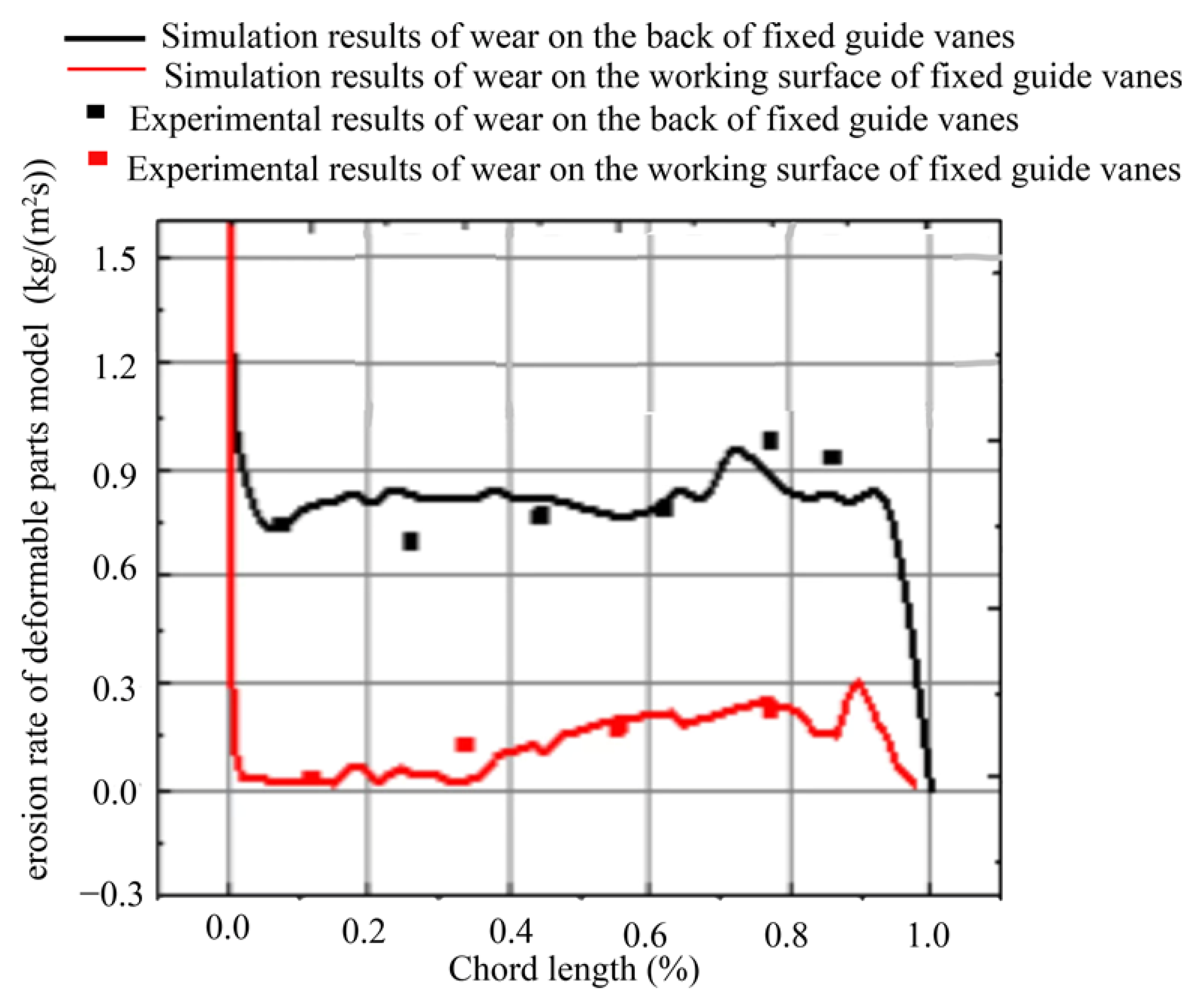
Thirdly, the DPM is used to conduct a two-phase flow simulation on the fixed guide vanes. This allows for the determination of the wear rate and velocity distribution of the guide vanes. The simulation results align well with the experimental results, indicating the effectiveness of the DPM model in simulating wear in the flow-through components of hydraulic turbines.
Lastly, this technology has been successfully applied in the design, manufacturing, and operation of wear-resistant hydraulic turbines at Xia Te Power Station in Xinjiang. Situated in a region with sediment-laden rivers, the power station has undergone one year of actual operation. Comparative analysis with similar power stations in the area confirms that the overall condition of the turbine’s runner, guide vanes, and other critical flow-through components at Xia Te Power Station is satisfactory, meeting the design and operational requirements for safe and stable unit operation.

Author Contributions

Conceptualization, X.L.; Methodology, Y.Z.; Investigation, W.H.; Writing—original draft, L.J. All authors have read and agreed to the published version of the manuscript.

Funding

This research is supported by the National Natural Science Foundation of China (approval No. 51279172), the Key Laboratory of Fluid and Power Machinery, Ministry of Education, Xihua University.

Data Availability Statement

The data sets presented in this study are available upon reasonable request to the corresponding author, as indicated on the first page.

Conflicts of Interest

The authors declare no conflict of interest. The funders had no role in the design of the study; in the collection, analyses, or interpretation of data; in the writing of the manuscript, or in the decision to publish the results.

Abbreviations

DPMDiscrete Phase Model
ttime variable (s)
Uvelocity
CFDComputational Fluid Dynamics
nabla operator
µdynamic viscosity
ρdensity
ggravitational acceleration (m s−2)
UGUnigraphics
Ødiameter
Ppressure (Pa)
ReReynolds number
µviscosity (kg m−1 s−1)

References

  1. Zhong, G.; Xu, B.; Xie, R.; Cheng, K.; Wu, C. The simulation analysis of the fracture liquid to the eroding and wear of the four-way tube. Mech. Sci. Technol. 2021, 40, 8. [Google Scholar]
  2. Chen, Z.; Yu, Y.; Fan, X. Vice roller mill grade screening research field. Comput. Simul. 2019, 36, 215–219+294. [Google Scholar]
  3. Liao, J.; Zhang, W.; Zhang, X. Numerical Analysis of Solid-Liquid Two-Phase Flow in the Runner of a Francis Turbine before and after Reconstruction. Hydraul. Power Gener. 2017, 43, 73–75. [Google Scholar]
  4. Lei, X. Research on Particle Scale Wear Model Based on Tangential Impact Energy and Its Application. Ph.D. Thesis, Zhejiang University, Zhejiang, China, 2019. [Google Scholar]
  5. Liu, H.; Mou, H. Study on erosion and wear of solid proppant on fracturing pipeline in sand fracturing. China Saf. Prod. Sci. Technol. 2018, 14, 87–94. [Google Scholar]
  6. Zhu, J.; Zhao, J. Analysis and Calculation of the Motion Trajectory of Solid Particles in an Impeller. Water Pump Technol. 1989, 3, 14–20. [Google Scholar]
  7. Li, R.; Liu, Y. A Mathematical Model for the Boundary Layer of Steady Solid-Liquid Two-Phase Flow. Fluid Mach. 2000, 28, 26–28. [Google Scholar]
  8. Cao, Y.; Li, R.; Gu, X. Boundary Element Analysis Method for Flow Field in Double Row Ring Cascades of Hydraulic Turbines. J. Lanzhou Univ. Technol. 1989, 8–17. [Google Scholar]
  9. Liu, X.; Cheng, L. Numerical simulation of solid liquid two-phase turbulence and particle wear. J. Water Conserv. 1996, 8, 20–27. [Google Scholar]
  10. Sheldon, G.L.; Finnie, I. On the Ductile Behavior of Nominally Brittle Materials During Erosive Cutting. J. Eng. Ind. 1966, 88, 387. [Google Scholar] [CrossRef]
  11. Hashemisohi, A.; Wang, L.; Shahbazi, A.; Amini, H. Numerical analysis and experimental validation of hydrodynamics of a thin bubb-ling fluidized bed for various particle-size distributions using a three-dimensional dense discrete phase model. Particuology 2020, 49, 191–204. [Google Scholar] [CrossRef]
  12. Jafari, A.; Dehghani, K.; Bahaaddini, K.; Hataie, R.A. Experimental comparison of abrasive and erosive wear characteristics of four wear-resistant steels. Wear 2018, 416, 14–26. [Google Scholar] [CrossRef]
  13. Singh, J.; Kumar, S.; Singh, J.P.; Kumar, P.; Mohapatra, S.K. CFD modeling of erosion wear in pipe bend for the flow of bottom ash suspension. Part. Sci. Technol. 2019, 137, 275–285. [Google Scholar] [CrossRef]
  14. Sato, J.; Usami, K.; Okamura, T.; Hokkirigawa, K. Comparision of silt erosion characteristics of materials through diferent types of test methods. In Proceedings of the 3rd Japan-China Joint Conference on Fluid Machinary, Osaka, Japan, 23–25 April 1990; pp. 201–207. [Google Scholar]
  15. Padhy, M.K.; Saini, R.P. A review on silt erosion in hydro turbines. Renew. Sustain. Energy Rev. 2008, 12, 1974–1987. [Google Scholar] [CrossRef]
  16. Sugiyama, K.; Nakahama, S.; Hattori, S.; Nakano, K. Slurry wear and cavitation erosion of thermal-sprayed cermets. Wear 2005, 258, 768–775. [Google Scholar] [CrossRef]
  17. Neppane, H.P. Sediment Erosion in Hydro Turbines. Ph.D. Thesis, Norwegian University of Science and Technology (NTNU), Trondheim, Norway, 2010. [Google Scholar]
  18. Thpa, B. Sand Erosion in Hydraulic Machinery. Ph.D. Thesis, Norwegian University of Science and Technology (NTNU), Trondheim, Norway, 2004. [Google Scholar]
  19. Laouari, A.; Ghenaiet, A. Investigation of steady and unsteady cavitating flows through a small Francis turbine. Renew. Energy 2021, 172, 841–861. [Google Scholar] [CrossRef]
  20. Yonezawa, K.; Watamura, T. Experimental and Numerical Investigations of Erosion on Runner Seal of a Francis Turbine. IOP Conf. Ser. Earth Environ. Sci. 2021, 774, 012034. [Google Scholar] [CrossRef]
  21. Noon, A.A.; Jabbar, A.U.; Koten, H.; Kim, M.-H.; Ahmed, H.W.; Mueed, U.; Shoukat, A.A.; Anwar, B. Strive to Reduce Slurry Erosion and Cavitation in Pumps through Flow Modifications, Design Optimization and Some Other Techniques: Long Term Impact on Process Industry. Materials 2021, 14, 521. [Google Scholar] [CrossRef]
  22. Chitrakar, S.; Dahlhaug, O.G.; Neopane, H.P. Numerical investigation of the effect of leakage flow through erosion-induced clearance gaps of guide vanes on the performance of Francis turbines. Eng. Appl. Comput. Fluid Mech. 2018, 12, 662–678. [Google Scholar] [CrossRef]
  23. Thapa, B.S.; Dahlhaug, O.G.; Thapa, B. Sediment erosion induced leakage flow from guide vane clearance gap in a low specific speed Francis turbine. Renew. Energy 2017, 107, 253–261. [Google Scholar] [CrossRef]
  24. Finnie, I. Erosion of surfaces by solid particles. Wear 1960, 3, 87–103. [Google Scholar] [CrossRef]
  25. Haugen, K.; Kvernvold, O.; Ronold, A.; Sandberg, R. Sand erosion of wear-resistant materials: Erosion in choke valves. Wear 1995, 186-187, 179–188. [Google Scholar] [CrossRef]
  26. Celik, I.; Ghia, U.; Roache, P.; Freitas, C.; Coleman, H.; Raad, P. Procedure for estimation and reporting of uncertainty due to discretization in CF. J. Fluids Eng. Trans. ASME 2008, 130, 078001. [Google Scholar]
Figure 1. Overall 3D diagram of hydraulic turbine. (a) Overall three-dimensional model diagram of hydraulic turbine; (b) 3D exploded view of hydraulic turbine.
Processes 11 02117 g001
Figure 2. 3D view of fixed guide vane.
Processes 11 02117 g002
Figure 3. Grid diagram of fixed guide vane.
Processes 11 02117 g003
Figure 4. Partial enlarged grid diagram of fixed guide vane.
Processes 11 02117 g004
Figure 5. Schematic diagram of the runner design.
Processes 11 02117 g005
Figure 6. Grid diagram.
Processes 11 02117 g006
Figure 7. Pressure distribution diagram of guide vane.
Processes 11 02117 g007
Figure 8. Partial view of pressure distribution on the cross-section of the guide vane.
Processes 11 02117 g008
Figure 9. Sediment distribution on the upper surface of the water guiding mechanism.
Processes 11 02117 g009
Figure 10. Sediment distribution on the lower surface of the water guiding mechanism.
Processes 11 02117 g010
Figure 11. Pressure distribution around the high flow wall surface of fixed guide vane under design conditions.
Processes 11 02117 g011
Figure 12. Velocity distribution of sediment flow around the near wall surface of fixed guide vane under design conditions.
Processes 11 02117 g012
Figure 13. Distribution of sediment volume fraction around the near wall surface of the design flow guide vane.
Processes 11 02117 g013
Figure 14. Wear rate nephogram of fixed guide vane. (a) Working surface of fixed guide vane; (b) back surface of fixed guide vane.
Processes 11 02117 g014
Figure 15. Relationship between chord length and concentration of discrete phase and discrete phase velocity at the back of fixed guide vane.
Processes 11 02117 g015
Figure 16. System diagram of test device.
Processes 11 02117 g016
Figure 17. Photographs of test site.
Processes 11 02117 g017
Figure 18. Sectional machining drawing of working section. (a) Cross-sectional profile of the working section; (b) longitudinal profile of the working section.
Processes 11 02117 g018
Figure 19. Single passage diagram for guide vane wear test section.
Processes 11 02117 g019
Figure 20. Physical box of the test section.
Processes 11 02117 g020
Figure 21. Guide vane installation in the test section. (a) Before guide vane installation; (b) after guide vane installation.
Processes 11 02117 g021
Figure 22. Schematic diagram of space coordinate position of test piece.
Processes 11 02117 g022
Figure 23. White light interference profilometer.
Processes 11 02117 g023
Figure 24. Method for extracting the surface wear depth of the test specimen.
Processes 11 02117 g024
Figure 25. Comparison diagrams of fixed guide vane before and after wear. (a) Before wear; (b) after wear.
Processes 11 02117 g025
Figure 26. Distribution diagram of chordal wear of fixed guide vane airfoil.
Processes 11 02117 g026
Figure 27. Fitting curve between wear rate and flow velocity.
Processes 11 02117 g027
Figure 28. Comparison between simulated and experimental data of fixed guide vane wear rate.
Processes 11 02117 g028
Table 1. Grid independence analysis.
Grid Size (mm)Number of Grids
Option 10.074407228
Option 20.774006570
Option 30.08753305421
Option 40.1052754518
Option 50.142203614
Table 2. Basic parameters of sediment.
Median Particle Size of Sediment (mm)Sand Particle Density (kg·m−3)Sand Content (kg·m−3)Volume Fraction of Sand Particles
0.126509.270.0036
Table 3. Grain gradation of suspended sediment samples.
Particle size (mm)0.0020.0050.0750.250.5
Sand weight of less than the particle size14.526.875.098.3100
Table 4. Mineral composition of suspended sediment samples.
Mineral CompositionQuartzCalciteFeldsparChlorite
Proportion (%)66.919.19.84.2
Table 5. Working conditions of the model for various materials used in wear rate fit calculation equation.
MaterialCoefficient KIndex nFitting Equation for Wear Rate
Fixed guide vaneQ3453.20 × 10–52.7E = 3.20 × 10 − 5CVW2.7
Disclaimer/Publisher’s Note: The statements, opinions and data contained in all publications are solely those of the individual author(s) and contributor(s) and not of MDPI and/or the editor(s). MDPI and/or the editor(s) disclaim responsibility for any injury to people or property resulting from any ideas, methods, instructions or products referred to in the content.

