
Multi-Zone Integrated Iterative-Decoupling Control of Temperature Field of Large-Scale Vertical Quenching Furnaces Based on ESRNN


Abstract
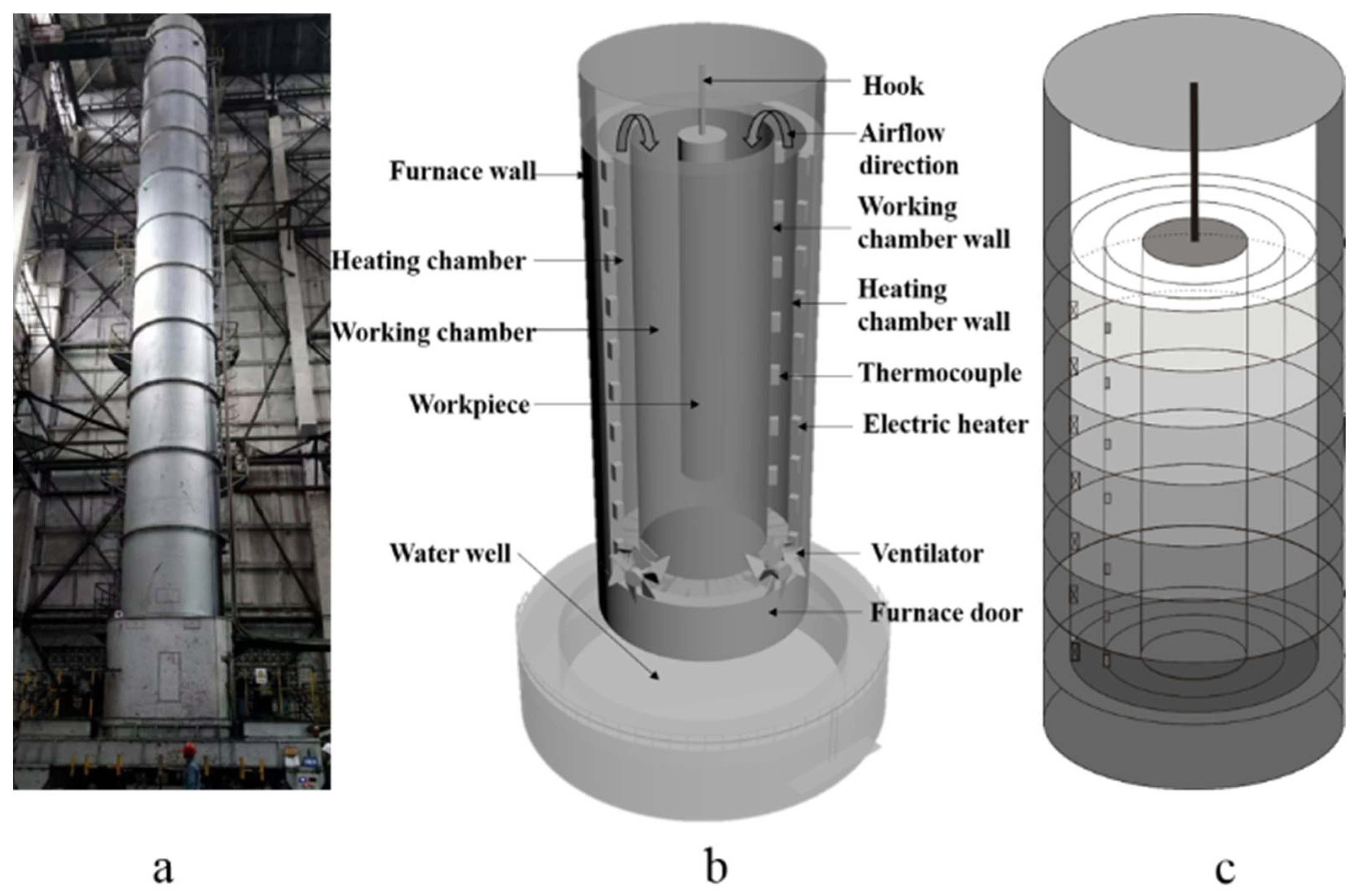
:1. Introduction
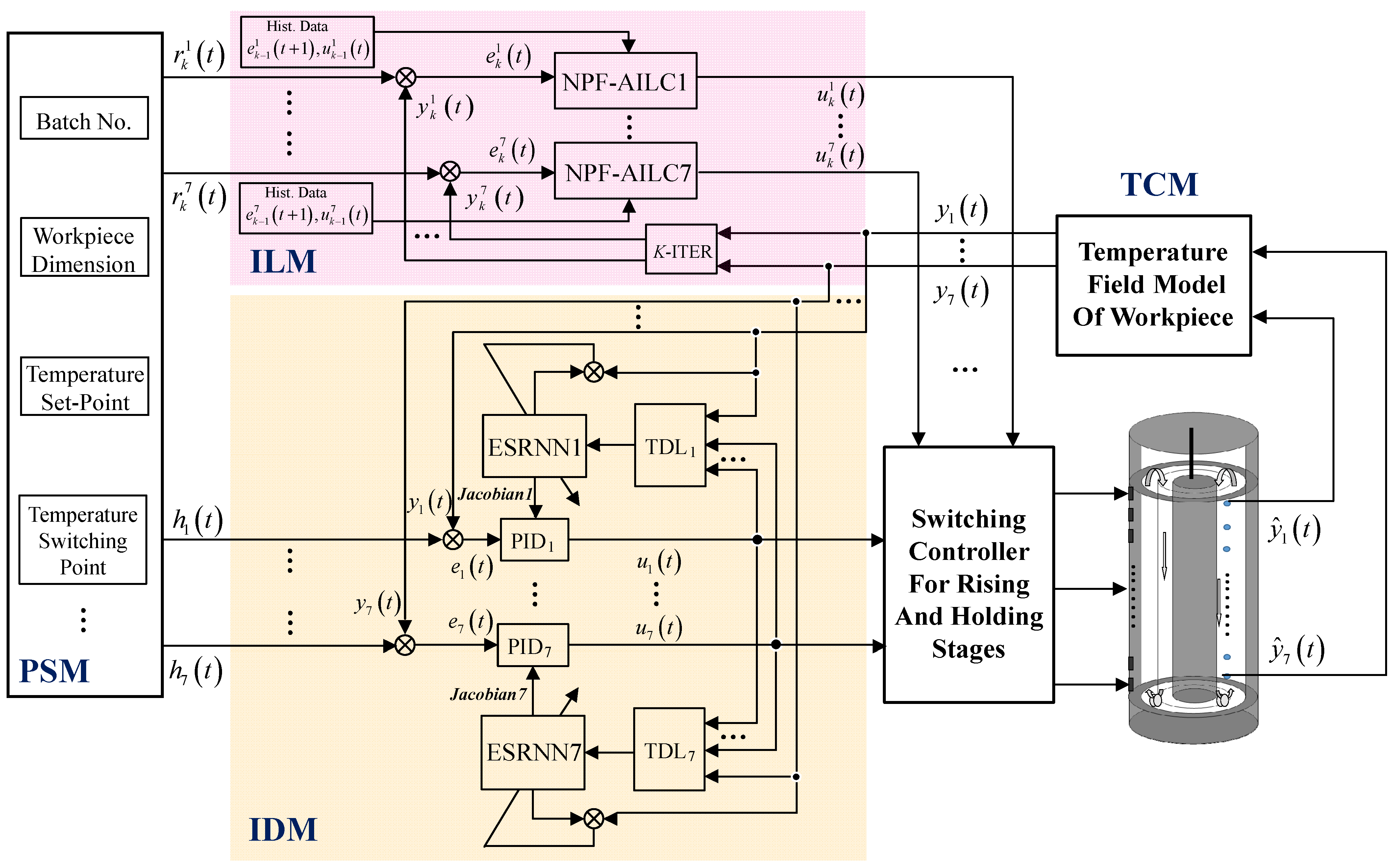
2. Methodology
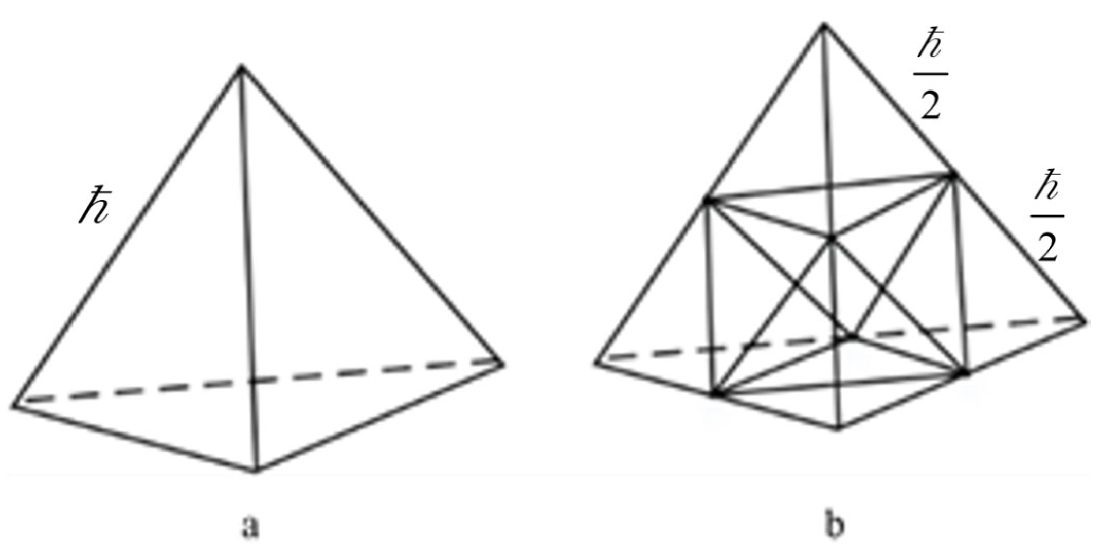
3. Workpiece Temperature Compensation Based on Spatial-Temporal Finite Extrapolation Method
3.1. Workpiece Temperature Model
3.2. Spatial-Temporal Finite Extrapolation Algorithm
4. Nonparametric Adaptive Iterative Control of Vertical Quenching Furnace Based on Self-Incentive
- (1)
- The partial derivative of with respect to the control input exists and is continuous;
- (2)
- For all and , when , the system of Equation (1) satisfies generalized continuity [35], that is, and ,where , and is a constant.
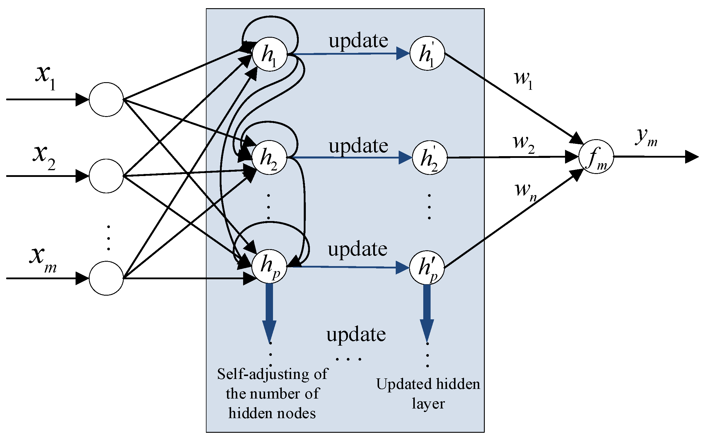
5. Integrated Intelligent Decoupling Control Based on ESRNN
5.1. Establishment of ESRNN
- Step 1: Initialize based on the characteristics of input samples and initialize the learning rate . For the first input sample, it is set as . Let the first cluster be and , the clustering center and the first hidden node is constructed.
- Step 2: When the th input data is collected, the number of samples is , . There have been clusters. The clustering centers and the hidden nodes are , . If , keep the current clustering result and the network structure unchanged, and go to Step 6. Otherwise, the network structure will be self-adapted. The number of the hidden-layer nodes is changed as , then go to Step 3.
- Step 3: The input matrix is centralized to , and calculate the eigenvectors of to obtain the feature space indicator vector of the cluster to which each sample belongs. All samples are re-clustered using Equations (38) and (39), yielding a new cluster set .
- Step 4: Use Equation (45) to update the clustering centers and combine with Equation (41) to concurrently update the width .
- Step 5: Use Equations (50)–(52) to update the weight vector of the network to complete the construction and training of ESRNN.
- Step 6: Use Equation (47), and the output is obtained as
- Step 7: End of the process until the temperature holding period is finished. Else, go to Step 2.
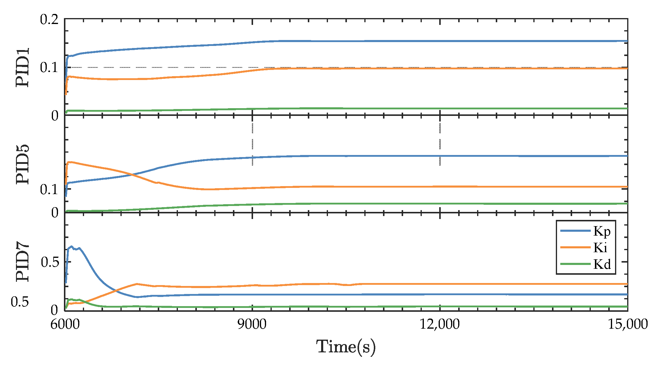
5.2. Integrated Intelligent Decoupling Controller
6. Simulation Results and Discussion
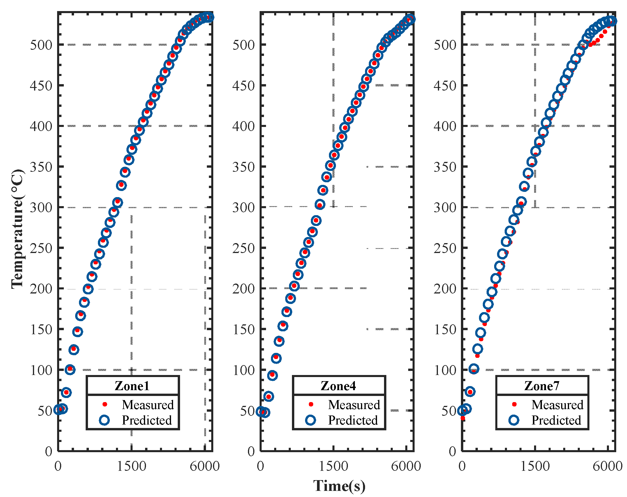
6.1. Model Verification
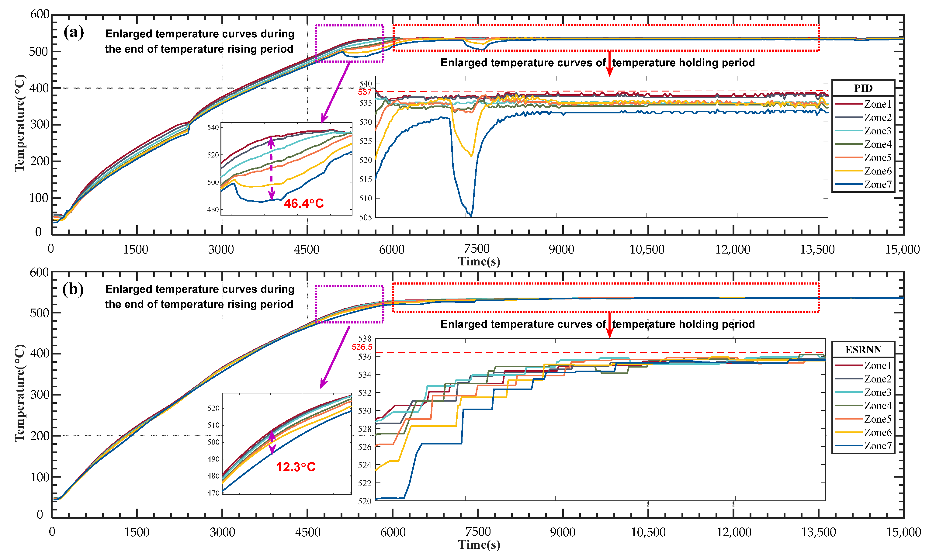
6.2. Validation of the Integrated Iterative-Decoupling Control
7. Conclusions
Author Contributions
Funding
Data Availability Statement
Conflicts of Interest
References
- Shen, L.; Chen, Z.; Jiang, Z.; He, J.; Yang, C.; Gui, W. Optimal Temperature Rise Control for a Large-Scale Vertical Quench Furnace System. IEEE Trans. Syst. Man Cybern. Syst. 2022, 52, 4912–4924. [Google Scholar] [CrossRef]
- Dang, W.; He, J. A Novel Control Strategy Based on Temperature Dynamic Decoupling and Belief Expert Rule Base for Large-scale Vertical Quench furnaces. In Proceedings of the 36th Chinese Control Conference, Dalian, China, 26–28 July 2017. [Google Scholar] [CrossRef]
- Li, Y.; Shi, X.; Zhang, Y.; Xue, J.; Chen, X.; Zhang, Y.; Ma, T. Numerical investigation on the gas and temperature evolutions during the spontaneous combustion of coal in a large-scale furnace. Fuel 2021, 287, 119557. [Google Scholar] [CrossRef]
- Crnomarkovic, N.; Belosevic, S.; Tomanovic, I.; Milicevic, A. New application method of the zonal model for simulations of pulverized coal-fired furnaces based on correction of total exchange areas. Int. J. Heat Mass Transf. 2020, 149, 119192. [Google Scholar] [CrossRef]
- Yi, Z.; Su, Z.; Li, G.; Yang, Q.; Zhang, W. Development of a double model slab tracking control system for the continuous reheating furnace. Int. J. Heat Mass Transf. 2017, 113, 861–874. [Google Scholar] [CrossRef]
- Bao, Q.; Zhang, S.; Guo, J.; Li, Z.; Zhang, Z. Multivariate linear-regression variable parameter spatio-temporal zoning model for temperature prediction in steel rolling reheating furnace. J. Process Control 2023, 123, 108–122. [Google Scholar] [CrossRef]
- Avantner, M.; Atudent, J.; Veselý, Z. Continuous walking-beam furnace 3D zonal model and direct thermal-box barrier based temperature measurement. Case Stud. Therm. Eng. 2020, 18, 100608. [Google Scholar] [CrossRef]
- Ji, W.; Li, G.; Wei, L.; Yi, Z. Modeling and determination of total heat exchange factor of regenerative reheating furnace based on instrumented slab trials. Case Stud. Therm. Eng. 2021, 24, 100838. [Google Scholar] [CrossRef]
- Ouyang, M.; Wang, Y.; Wu, F.; Lin, Y. Continuous Reactor Temperature Control with Optimized PID Parameters Based on Improved Sparrow Algorithm. Processes 2023, 11, 1302. [Google Scholar] [CrossRef]
- Gao, Q.; Pang, Y.; Sun, Q.; Liu, D.; Zhang, Z. Numerical analysis of the heat transfer of radiant tubes and the slab heating characteristics in an industrial heat treatment furnace with pulse combustion. Int. J. Therm. Sci. 2021, 161, 106757. [Google Scholar] [CrossRef]
- Tang, G.; Wu, B.; Bai, D.; Wang, Y.; Bodnar, R.; Zhou, C. CFD modeling and validation of a dynamic slab heating process in an industrial walking beam reheating furnace. Appl. Therm. Eng. 2018, 132, 779–789. [Google Scholar] [CrossRef]
- López, Y.; Obando, J.; Echeverri-Uribe, C.; Amell, A.A. Experimental and numerical study of the effect of water injection into the reaction zone of a flameless combustion furnace. Appl. Therm. Eng. 2022, 213, 118634. [Google Scholar] [CrossRef]
- Casal, J.M.; Porteiro, J.; Míguez, J.L.; Vázquez, A. New methodology for CFD three-dimensional simulation of a walking beam type reheating furnace in steady state. Appl. Therm. Eng. 2015, 86, 69–80. [Google Scholar] [CrossRef]
- Tang, X.; Xu, B.; Xu, Z. Reactor Temperature Control Based on Improved Fractional Order Self-Anti-Disturbance. Processes 2023, 11, 1125. [Google Scholar] [CrossRef]
- Strommer, S.; Niederer, M.; Steinboeck, A.; Jadachowski, L.; Kugi, A. Nonlinear Observer for Temperatures and Emissivities in a Strip Annealing Furnace. IEEE Trans. Ind. Appl. 2017, 53, 2578–2586. [Google Scholar] [CrossRef]
- Tan, Y.; Zhou, M.; Wang, Y.; Guo, X.; Qi, L. A Hybrid MIP–CP Approach to Multistage Scheduling Problem in Continuous Casting and Hot-Rolling Processes. IEEE Trans. Autom. Sci. Eng. 2019, 16, 1860–1869. [Google Scholar] [CrossRef]
- Seo, M.; Ban, J.; Cho, M.; Koo, B.Y.; Kim, S.W. Low-Order Model Identification and Adaptive Observer-Based Predictive Control for Strip Temperature of Heating Section in Annealing Furnace. IEEE Access 2021, 9, 53720–53734. [Google Scholar] [CrossRef]
- Yang, Y.; Shi, X.; Liu, X.; Li, H. A novel MDFA-MKECA method with application to industrial batch process monitoring. IEEE/CAA J. Autom. Sin. 2020, 7, 1446–1454. [Google Scholar] [CrossRef]
- Steinboeck, A.; Graichen, K.; Wild, D.; Kiefer, T.; Kugi, A. Model-based trajectory planning, optimization, and open-loop control of a continuous slab reheating furnace. J. Process Control 2011, 21, 279–292. [Google Scholar] [CrossRef]
- Steinboeck, A.; Wild, D.; Kugi, A. Nonlinear model predictive control of a continuous slab reheating furnace. Control Eng. Pract. 2013, 21, 495–508. [Google Scholar] [CrossRef]
- Suzuki, M.; Katsuki, K.; Imura, J.; Nakagawa, J.; Kurokawa, T.; Aihara, K. Simultaneous optimization of slab permutation scheduling and heat controlling for a reheating furnace. J. Process Control 2014, 24, 225–238. [Google Scholar] [CrossRef]
- Strommer, S.; Niederer, M.; Steinboeck, A.; Kugi, A. Hierarchical nonlinear optimization-based controller of a continuous strip annealing furnace. Control Eng. Pract. 2018, 73, 40–55. [Google Scholar] [CrossRef]
- Prinz, K.; Steinboeck, A.; Kugi, A. Optimization-based feedforward control of the strip thickness profile in hot strip rolling. J. Process Control 2018, 64, 100–111. [Google Scholar] [CrossRef]
- Schausberger, F.; Steinboeck, A.; Kugi, A. Feedback Control of the Contour Shape in Heavy-Plate Hot Rolling. IEEE Trans. Control Syst. Technol. 2017, 26, 842–856. [Google Scholar] [CrossRef]
- Du, S.; Wu, M.; Chen, X.; Cao, W. An intelligent control strategy for iron ore sintering ignition process based on the prediction of ignition temperature. IEEE Trans. Ind. Electron. 2020, 67, 1233–1241. [Google Scholar] [CrossRef]
- Zhou, H.; Deng, H.; Duan, J. Hybrid Fuzzy Decoupling Control for a Precision Maglev Motion System. IEEE/ASME Trans. Mechatron. 2018, 23, 389–401. [Google Scholar] [CrossRef]
- Zhang, J.; Feng, T.; Zhang, H.; Wang, X. The Decoupling Cooperative Control with Dominant Poles Assignment. IEEE Trans. Syst. Man Cybern. Syst. 2022, 52, 1205–1213. [Google Scholar] [CrossRef]
- Feng, Y.; Wu, M.; Chen, L.; Chen, X.; Cao, W.; Du, S.; Pedrycz, W. Hybrid Intelligent Control Based on Condition Identification for Combustion Process in Heating Furnace of Compact Strip Production. IEEE Trans. Ind. Electron. 2022, 69, 2790–2800. [Google Scholar] [CrossRef]
- Li, X.; Fang, Y.; Liu, L. Decoupling predictive control of strip flatness and thickness of tandem cold rolling mills based on convolutional neural network. IEEE Access 2020, 8, 3656–3667. [Google Scholar] [CrossRef]
- Zhang, H.; Jiang, Z.; Cheng, Z.; Gui, W.; Xie, Y.; Yang, C. Two-Stage Control of Endpoint Temperature for Pebble Stove Combustion. IEEE Access 2019, 7, 625–640. [Google Scholar] [CrossRef]
- Steinboeck, A.; Wild, D.; Kiefer, T.; Kugi, A. A mathematical model of a slab reheating furnace with radiative heat transfer and non-participating gaseous media. Int. J. Heat Mass Transf. 2010, 53, 5933–5946. [Google Scholar] [CrossRef]
- Matviychuk, A.R.; Parshikov, G.V.; Zimovets, A.A. On some method of constructing the reachability set in Rn. IFAC-PapersOnLine 2015, 48, 223–226. [Google Scholar] [CrossRef]
- Meštrović, M.; Ocvirk, E. An application of Romberg extrapolation on quadrature method for solving linear Volterra integral equations of the second kind. Appl. Math. Comput. 2007, 194, 389–393. [Google Scholar] [CrossRef]
- Richards, S.A. Completed Richardson extrapolation in space and time. Commun. Numer. Methods Eng. 1997, 13, 573–582. [Google Scholar] [CrossRef]
- Martire, A.L. Volterra integral equations: An approach based on Lipschitz-continuity. Appl. Math. Comput. 2022, 435, 127496. [Google Scholar] [CrossRef]
- Treesatayapun, C. Model free adaptive control with pseudo partial derivative based on fuzzy rule emulated network. In Proceedings of the 2012 International Conference on Artificial Intelligence (ICAI), Las Vegas, NV, USA, 16–19 July 2012; The Steering Committee of the World Congress in Computer Science, Computer Engineering and Applied Computing (WorldComp): Las Vegas, NV, USA, 2012. [Google Scholar]
- Gutman, I.; Martins, E.A.; Robbiano, M.; San Martín, B. Ky Fan theorem applied to Randić energy. Linear Algebra Appl. 2014, 459, 23–42. [Google Scholar] [CrossRef]


| Index/% Zone | MRE 1 | RRMSE 2 |
|---|---|---|
| Zone 1 | 0.3195 | 0.0054 |
| Zone 4 | 0.3268 | 0.0052 |
| Zone 7 | 0.5288 | 0.0105 |
| Index | Conventional | Proposed |
|---|---|---|
| Max Deviation (°C) | 3.3000 | 1.1702 |
| Average Deviation (°C) | 2.5088 | 0.5272 |
| Max Overshoot (%) | 0.6168 | 0.2187 |
| Average Overshoot (%) | 0.4689 | 0.0985 |
| Mean Static Error (°C) | 1.1664 | 0.4946 |
| Average Tuning Time (×104 s) | 1.3100 | 1.2500 |
| Max Steady State Error (°C) | 5.9000 | 1.7000 |
| Average Steady State Error (°C) | 1.1375 | 0.4458 |
Disclaimer/Publisher’s Note: The statements, opinions and data contained in all publications are solely those of the individual author(s) and contributor(s) and not of MDPI and/or the editor(s). MDPI and/or the editor(s) disclaim responsibility for any injury to people or property resulting from any ideas, methods, instructions or products referred to in the content. |
© 2023 by the authors. Licensee MDPI, Basel, Switzerland. This article is an open access article distributed under the terms and conditions of the Creative Commons Attribution (CC BY) license (https://creativecommons.org/licenses/by/4.0/).
Share and Cite
Shen, L.; Chen, Z.; He, J. Multi-Zone Integrated Iterative-Decoupling Control of Temperature Field of Large-Scale Vertical Quenching Furnaces Based on ESRNN. Processes 2023, 11, 2106. https://doi.org/10.3390/pr11072106
Shen L, Chen Z, He J. Multi-Zone Integrated Iterative-Decoupling Control of Temperature Field of Large-Scale Vertical Quenching Furnaces Based on ESRNN. Processes. 2023; 11(7):2106. https://doi.org/10.3390/pr11072106
Chicago/Turabian StyleShen, Ling, Zhipeng Chen, and Jianjun He. 2023. "Multi-Zone Integrated Iterative-Decoupling Control of Temperature Field of Large-Scale Vertical Quenching Furnaces Based on ESRNN" Processes 11, no. 7: 2106. https://doi.org/10.3390/pr11072106
APA StyleShen, L., Chen, Z., & He, J. (2023). Multi-Zone Integrated Iterative-Decoupling Control of Temperature Field of Large-Scale Vertical Quenching Furnaces Based on ESRNN. Processes, 11(7), 2106. https://doi.org/10.3390/pr11072106