Application and Comparison of Machine Learning Methods for Mud Shale Petrographic Identification

Abstract

Machine learning is the main technical means for lithofacies logging identification. As the main target of shale oil spatial distribution prediction, mud shale petrography is subjected to the constraints of stratigraphic inhomogeneity and logging information redundancy. Therefore, choosing the most applicable machine learning method for different geological characteristics and data situations is one of the key aspects of high-precision lithofacies identification. However, only a few studies have been conducted on the applicability of machine learning methods for mud shale petrography. This paper aims to identify lithofacies using commonly used machine learning methods. The study employs five supervised learning algorithms, namely Random Forest Algorithm (RF), BP Neural Network Algorithm (BPANN), Gradient Boosting Decision Tree Method (GBDT), Nearest Neighbor Method (KNN), and Vector Machine Method (SVM), as well as four unsupervised learning algorithms, namely K-means, DBSCAN, SOM, and MRGC. The results are evaluated using the confusion matrix, which provides the accuracy of each algorithm. The GBDT algorithm has better accuracy in supervised learning, while the K-means and DBSCAN algorithms have higher accuracy in unsupervised learning. Based on the comparison of different algorithms, it can be concluded that shale lithofacies identification poses challenges due to limited sample data and high overlapping degree of type distribution areas. Therefore, selecting the appropriate algorithm is crucial. Although supervised machine learning algorithms are generally accurate, they are limited by the data volume of lithofacies samples. Future research should focus on how to make the most of limited samples for supervised learning and combine unsupervised learning algorithms to explore lithofacies types of non-coring wells.

1. Introduction

With the breakthroughs in the exploration and development of marine shale reservoirs in North America, developing unconventional oil and gas has become a hot topic; many countries have started to invest in the unconventional aspects of oil and gas, focusing on the exploration of hydrocarbon rock systems [1]. Petrography is a feature of rocks or rock assemblages formed in a certain sedimentary environment and the main component of sedimentary phases, including color, composition, structure, and sedimentary structure. Many scholars have focused on the mineral composition of different lithofacies types and the evolutionary history of lake basins; meanwhile, studies on the accurate identification and delineation of petrography are lacking [2]. At present, the classification of mud shale lithofacies phases is mainly based on the test results of various experimental analyses (such as core observation, rock thin section, spring X diffraction, principal element analysis, specular body reflectance, total organic carbon content, conventional rock pyrolysis, fluid inclusions, and electron microprobe), on the mineral characteristics [3], formation environment [4], diagenesis [5], elemental geochemical characteristics [6], and other features of mud shale to comprehensively classify its lithofacies types. Most current studies focus on individual shale samples, leading to identification, prediction, promotion, and application difficulties and the inability to quickly and precisely clarify shale oil’s favorable formation and spatial distribution characteristics in the whole region. As a basic unit reflecting rocks’ physical and chemical properties, petrography has the conditions to be promoted. Thus, the lithofacies delineation of mud shale has become important in exploring and evaluating shale oil.

Logging data are widely used in lithofacies identification and evaluation because of their high vertical resolution and continuity [7,8]. Zhang Jinyin [9] used the analytical data of systematic core wells to establish a model of fine lithofacies delineation based on the large-scale lithologic changes (described by core logging) and minute-scale (described by experimental analysis) lithologic features of mud shale, scaled imaging log information, and established a model of fine lithofacies delineation by calibrating conventional log data with color scale changes on imaging maps for the identification and delineation of mud shale petrography. Chao Zhang et al. [10] established a model of fine lithofacies delineation by selecting logging curves, such as GR (Natural gamma rays), AC (Acoustic time logging curve), and CNL (compensated neutron logging), to achieve lithofacies delineation. Yan et al. [11] applied core description, thin section observation, electron microscope imaging, and nuclear magnetic resonance to study the lithofacies characteristics of mud shale; they combined the results with logging data to identify the laminae structure and calculate geochemical parameters, such as total organic carbon content and pyrolysis hydrocarbon content (S2), and established a method of mud shale lithofacies identification based on log data. Shiqi Che [12] established a three-terminal meta-plate of shale mineral fractions based on ECS logging and rock thin section data to realize the division of shale lithofacies phases and then combined the results with conventional logging data to establish a logging identification plate. Yang Yang et al. [13] constructed a shale lithofacies identification radar plate and used logging data and core test data to establish multiparameter preference and multivariate linear fitting, respectively, in the prediction equations for the relative contents of clay minerals and siliceous minerals. Wang Shengzhu [14] used reservoir characterization techniques, such as rock thin section, X-ray diffraction of whole rock mineral analysis, and field emission environmental scanning electron microscopy combined with organic geochemical test analysis, to classify lithofacies phases according to rock mineral components, laminar structure, organic carbon content, and other indicators.

The reservoir’s complexity and heterogeneity lead to information redundancy between logging curves and an unbalanced distribution of data sets. As a result, linear equations and empirical statistical formulas are insufficient in describing shale lithofacies. To address this issue, scholars have turned to machine learning algorithms [15,16,17] for lithofacies identification. This approach not only reduces interpretation costs but also improves analysis effectiveness. Machine learning algorithms used in shale facies recognition can be categorized into three types: supervised learning, unsupervised learning, and reinforcement learning. These categories are determined based on the different training samples and feedback methods used in the algorithms. The first two categories, supervised and unsupervised learning, are the most commonly used in shale facies recognition. Supervised learning algorithms are widely used in petrology to analyze basic data. In basins where lithofacies standards are established in rock cores, these algorithms can provide lithofacies petrophysical characteristics to help establish training models. Commonly used methods include nonlinear regression analysis (BPANN), nearest neighbor (KNN), decision tree (DT), and vector machine (SVM). Naive Bayes (NB) is less frequently used due to difficulties in handling interfering data sets [18,19,20,21]. Naive Bayes (NB) is seldom used because it is difficult to deal with data sets that interfere with each other [22,23]. In 2016, Bhattacharya et al. used the vector machine method to identify the lithofacies of Marcellus Shale, USA, and in 2018 applied Bayesian Network Theory and Random Forest to predict the presence of different facies and fractures in sedimentary rocks using common well logs. Supervised machine learning models using Bayesian Network Theory and Random Forest were established to classify facies and fractures in unconventional shale, conventional sandstone, and carbonate reservoirs. In addition to the above single machine learning algorithm, many scholars use multi-algorithm fusion to establish lithofacies recognition models [24,25,26]. Wang (2020) combined the hidden Markov model and random forests, proposing a novel method for lithology identification [25]. The sample space was expanded through the intrinsic relationship of the petrophysical properties, thereby improving the accuracy of lithofacies division. The accuracy of the unsupervised learning algorithm in shale reservoir prediction is effectively improved by continuously expanding the training samples. This algorithm has proven to be effective for new exploration basins with limited core samples and petrophysical data. In Al-Mudhafar et al. (2019) [27], a K-means clustering algorithm was implemented as a statistical solution to classify reservoir facies given well logs and core data in a reservoir from the south of Iraq. The data included well log records such as GR, SP, Density, Neutron Porosity, Total Porosity, Resistivity, Induction, Shale Volume, Water Saturation, along with porosity and permeability values from core analysis. Nafees 2023 used the self-organizing map (SOM) for the recognition of lithofacies and successfully extended this application to non-cored wells. It solves the problem that supervised learning algorithms cannot identify lithofacies from coreless data [28]. In the field of lithofacies identification, unsupervised machine learning algorithms such as model-based clustering, K-means clustering, ward hierarchical partitioning, and SOM have been extensively utilized [29]. Researchers have also conducted an applicability analysis of various algorithms in lithofacies identification [30,31,32]. In a study conducted by Wang Min in 2023, the division effect of shale lithofacies was compared using KNN, SVM, XG-Boots, and RF. Li Chang also explored the applicability of lithofacies division among SOM, MRGC, and KNN in 2021. While ANN was compared, the comparison was limited to either a supervised learning algorithm or both supervised and unsupervised learning algorithms. As the supervised learning algorithm utilizes a more accurate training set established by petrophysics, the division results were found to be superior to those obtained using unsupervised learning algorithms.

This paper presents a classification of shale lithofacies types in the Bohai Bay Basin based on organic matter abundance, rock type, and mineral composition. The study then compares the effectiveness of different machine algorithms for lithofacies classification using logging identification. The aim is to optimize the machine learning algorithm suitable for shale lithofacies classification in basins with different exploration degrees and provide a basis for subsequent shale reservoir exploration and evaluation. However, the accuracy of the comparison remains to be discussed.

2. Methods and Materials

2.1. Materials

This study focuses on the distribution and classification of lacustrine oil shale in the A section of a depression in Bohai Bay Basin. The researchers use data samples from two coring wells and combine them with core observation and analysis test results to identify shale types. They analyze conventional logging curves such as GR, SP, RT, AC, CNL, and DEN to compare the effectiveness of supervised and unsupervised learning algorithms in shale lithofacies logging identification.

2.2. Methods

2.2.1. Supervised Learning Algorithm

1.

BPANN algorithm

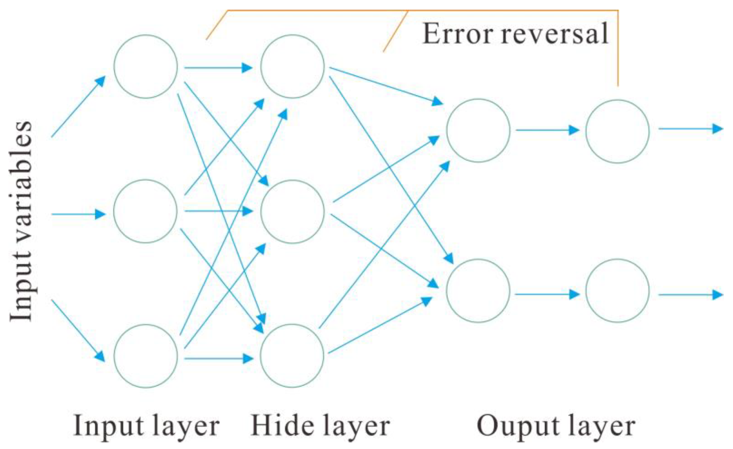
BPANN is a multilayer feedforward network that propagates according to reverse errors using a dual mechanism of learning signal forward propagation and error backpropagation to train data. The BP algorithm takes the square of network error as the objective function and uses the gradient descent method to calculate the minimum value of the objective function [33,34]. Figure 1 shows a typical basic neural network structure. Each part of the structure plays its role; the input layer is mainly responsible for receiving information transmitted from the outside world, and the output layer serves as the output part of the processed structure of the output system. The hidden layer with the most important role is located between the input and output layers and is mainly responsible for processing the external information transmitted by the input layer. We plan to establish a production capacity prediction model using the BP neural network model, a classic and important forward network model. The two important principles of the BP neural network model are forward data transmission and error feedback correction, as shown in Figure 1.

In the forward broadcast of Figure 2, the input of information transmitted by other neurons to this neuron enters the input part of the neuron structure. The calculation amount is determined and transmitted to the hidden layer by connecting the weights and adding the neuron threshold. The neurons in the hidden layer undergo repeated calculations to obtain variables and pass them on to the next layer, the output layer. At this point, most of the forward delivery phase has been completed. The input layer that receives the transmitted signal compares the expected output value with the calculated output value. After being calculated, the resulting error is transmitted back to the input layer, and the weight and threshold of the output layer are continuously adjusted, followed by a cyclic calculation. The loop calculation ends and outputs the result after the calculation error value is less than the expected error set by the model establishment. The above is the process of error inversion correction.

2.

RF algorithm

RF as an ensemble learning algorithm, which uses decision trees to train samples and aggregate prediction results through voting, thereby improving the model’s prediction accuracy. Its implementation is simple, and it performs well on multifeature data and data partially missing features, making it widely used in machine learning.

The RF algorithm is a combination classifier algorithm that uses a CART decision tree as the base classifier. It constructs a decision tree from the random sample sets with and without placement. The final multiple decision trees form an RF model whose final prediction result is determined by the base classifier’s vote. For classification, a decision tree is constructed by randomly selecting samples and sample features from the dataset. This process is repeated multiple times, and the resulting decision trees are uncorrelated. The results of all decision trees are counted as the final result. The classification results of each decision tree in the forest are counted for predicting new samples, and the most common category is selected as the new sample prediction result.

3.

GBDT algorithm

GBDT is a machine learning model with excellent predictive power. The residuals between the calculated and target values are quickly categorized and analyzed by regression trees and then continuously reduced using a step-up algorithm so that the calculated value gradually approaches the target value. This method is flexible in handling various data types and achieves high prediction accuracy with a short tuning time. Given that the regression tree handles various residual values differently, the training results will not be affected even when the sample has incorrect sample points. The core idea of the GBDT algorithm uses the negative gradient value of the loss function as an approximation of the loss value of the base model in multiple base models. This approximation is then applied to construct the base model in the next round, simplifying the solution of the objective function. The steps of GBDT implementation are shown in Figure 3.

This model uses the Python language to write the model program and the Sklearn module within the machine learning library to perform the modeling analysis. The main adjustment parameters of the model are the boosting framework parameters and weak learner parameters. The important parameters of the boosting framework include the maximum number of iterations, weight reduction factor, and loss function. The main parameters of the weak learner include the maximum number of features, the maximum depth of the decision tree, and the minimum number of samples of leaf nodes. For good results, the prediction model’s parameters must be adjusted before building the model. In choosing parameters, too few iterations easily result in underfitting; too small a learning rate requires a complex iterative process and a great computational effort; and too large a leaf node depth results in model overfitting. Therefore, the cross-validation method is used to determine a reasonable parameter system. The principle of parameter selection is mainly applied to the accuracy rate to judge the good or bad model fitting and to achieve a high accuracy rate by continuously adjusting the appropriate parameters.

4.

K Nearest Neighbor (KNN)

The K nearest neighbor classification algorithm (k Nearest Neighbor, KNN) is one of the simplest mathematical classification recognition algorithms. Each sample can be represented by its nearest k neighbors, and new samples can be directly classified according to the previous classification of the data set, without learning and training. If the neighbor of a sample to be divided is an object that has been correctly classified, then the category of the sample to be divided is determined according to the category of the nearest one or several samples. Therefore, the KNN method is not affected by outliers, and is suitable for classification problems with a large number of overlapping sample sets or cross-class domains [35]. The algorithm of the KNN method is simple and direct, and it can also be classified when the sample size is small or the sample features are few, but the number of sample types is required to be balanced.

5.

Support vector machine (SVM)

The Support Vector Machine (SVM) is a statistical method that can be applied to linear and nonlinear regression problems. It enhances the generalization ability of the learning machine by minimizing the empirical risk and confidence range, while seeking the minimum structured risk. This approach allows for the acquisition of good statistical laws even when working with a small number of statistical samples. The SVM achieves this by mapping the input space to a feature space through a nonlinear transformation. This transformation allows for the decision hypersurface model in the input space to correspond to decision hyperplane models in the feature space.

2.2.2. Unsupervised Learning Algorithm

6.

K-means

The K-means algorithm is a popular clustering method due to its high computational efficiency. It is commonly used for large-scale data clustering. The algorithm works by setting k as a parameter, determining the number of categories k that the data set containing n objects needs to be divided into. K objects are randomly selected as the initial clustering center, and then for each remaining object, the distance from the object to each initial cluster center is calculated using the distance formula. The objects are then divided into the nearest classes, and the class centers are recalculated. This process is repeated until the criterion function converges.

7.

DBSCAN

The DBSCAN algorithm is a density-based clustering method that identifies clusters as the largest set of density-connected points. By dividing areas with sufficient density into clusters, it can find clusters with arbitrary shapes in noisy spatial data sets. A cluster in DBSCAN can have one or more core points. If there is only one core point, all other non-core point samples in the cluster are in the Eps neighborhood of this core point. If there are multiple core points, there must be another core point in the Eps neighborhood of any core point in the cluster; otherwise, the two core points cannot be reached in density. The collection of all samples in the Eps neighborhood of these core points constitutes a DBSCAN cluster.

8.

SOM

Self-organizing mapping neural network is a kind of unsupervised training neural network, which realizes self-organizing and unsupervised learning by introducing the concept of neighborhood function, that is, all neurons are placed in a topology determined in advance according to prior knowledge. The introduction of neighborhood function makes the topological structure restrict SOM training, which can ensure that the training will not fall into a local minimum to the maximum extent [36]. It adopts a two-dimensional SOM structure, which consists of an input layer and competition layer. The dimension of the input layer is consistent with the dimension of the input sample vector, and the nodes in the competition layer are generally distributed in a two-dimensional array, and one node in the competition layer represents a neuron, and each neuron is connected by lateral inhibition, and the input layer and the competition layer are fully connected [37,38,39,40].

9.

MRGC

Image-based multi-resolution graph-based clustering (MRGC) is a method that utilizes nonparametric K-nearest neighbor and graphic data representation for multi-dimensional lattice image recognition. Unlike other methods, MRGC does not rely on the classification domain to determine the category, but rather on the limited adjacent samples around it. This makes it more suitable for core sample sets with overlapping or overlapping domains. In MRGC, the similarity between sampling points is measured using Euclidean distance, and the relationship between attraction and attraction between sampling points is determined based on the Euclidean distance matrix. In order to determine the attraction center of each sampling point, the nearest neighbor index (NI) is used to evaluate the ability of each point to attract other points. The sampling point with the highest NI value is selected as the final attraction center. The sample set is then divided into multiple attractive sets, with each set represented by a kernel representative index (KRI). The classification number for each level in the multi-level classification is determined by the descending order of the KRI values. Finally, the multi-level attractive sets are merged to obtain the final classification result [41].

3. Results

3.1. Division of Mud Shale Lithofacies Types

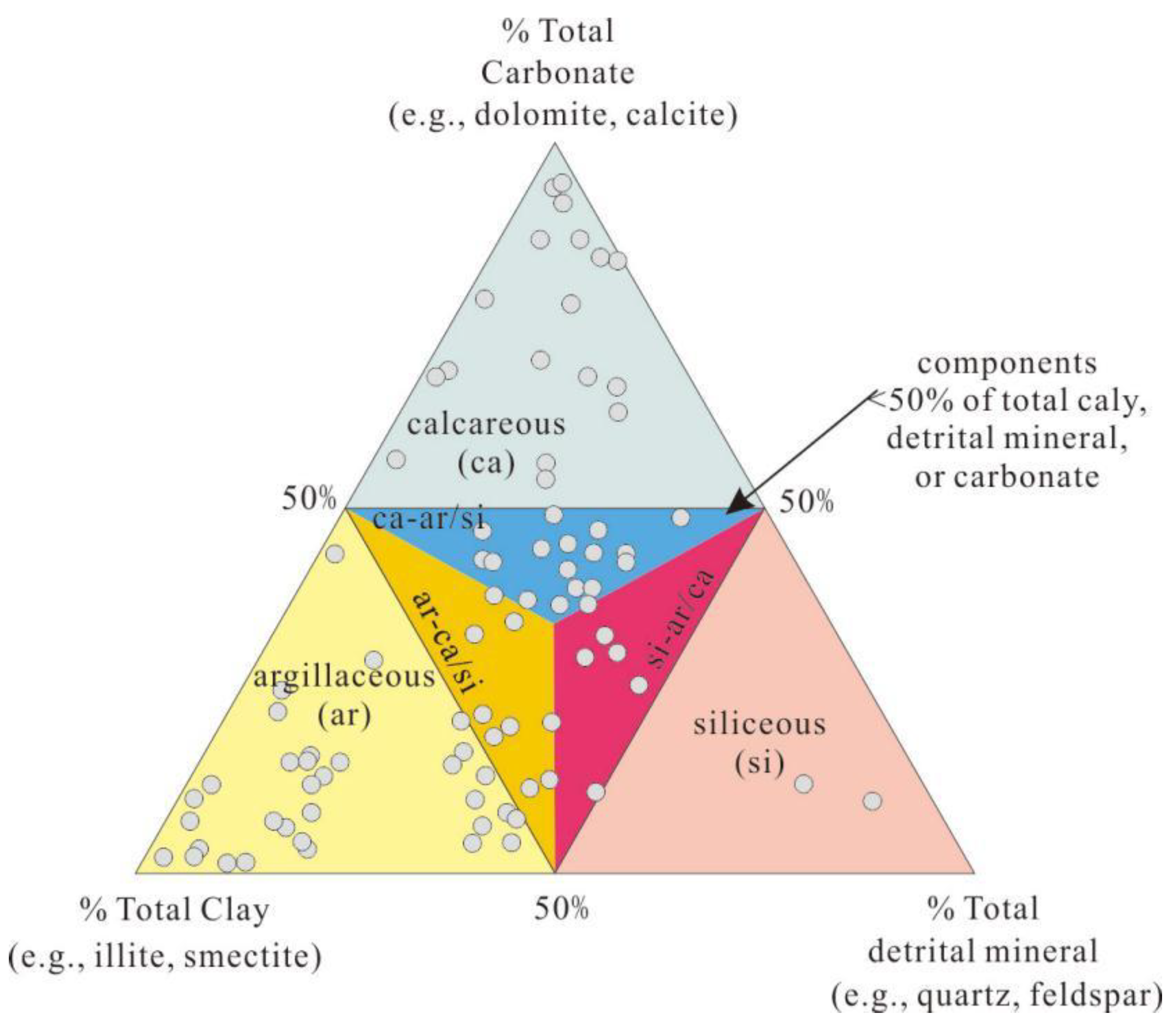
The mud shale strata in the Liaohe Depression, located in the northeast Bohai Bay basin, represent a typical mixed sedimentary sequence that has formed due to the combined effects of mechanical and chemical sedimentation of land-derived debris. The coexistence of various types of rocks, such as shale, mudstone, dolomitic mudstone, and dolomite, results in considerable variations in composition, structural features, and organic matter abundance. Different types of mud shale rocks can be effectively distinguished through classification based on the lithofacies of fine-grained sedimentary rocks. Mineral composition, sedimentary structure, and organic matter abundance are the frequently employed classification indicators for the lithofacies of fine-grained sedimentary rocks [42,43,44,45,46]. For the crucial step of rock naming, this paper adheres to existing research findings and adopts a three-end-member petrological classification [47,48,49,50]; clay minerals, felsic minerals (land-derived debris), and carbonate minerals (primarily dolomite) are considered as the three end members. Based on a 50% threshold, these rocks are categorized into four main types, as shown in Figure 1: clayey, felsic, dolomitic, and mixed. Considering the variations in organic matter content and occurrence state among different lithofacies of mudstone in the study area, those exhibiting total organic carbon (TOC) contents > 2% are classified as organic-rich mud shale, whereas those with TOC contents < 2% are referred to as organic-poor mud shale [51,52]. In terms of sedimentary structure parameters, stratification serves as one of the most important features of fine-grained sedimentary rocks [53]. This paper integrates the stratification scale parameters employed by various researchers for lithofacies classification to summarize stratification scales and names. They are distinguished from conventional rocks in terms of macroscopic massive (>1 m) and layered structures (subdivided based on the scale: 0.5–1 m thick layers, 0.1–0.5 m medium layers, 0.01–0.1 m thin layers, and <0.01 m shaly layers). The term ‘laminae’ (<1 mm, primarily concentrated within the 0.01–0.5 mm range) is introduced to describe the stratification of the meso-microstructure of fine-grained sedimentary rocks, and laminae may also be present in rocks with massive structures.

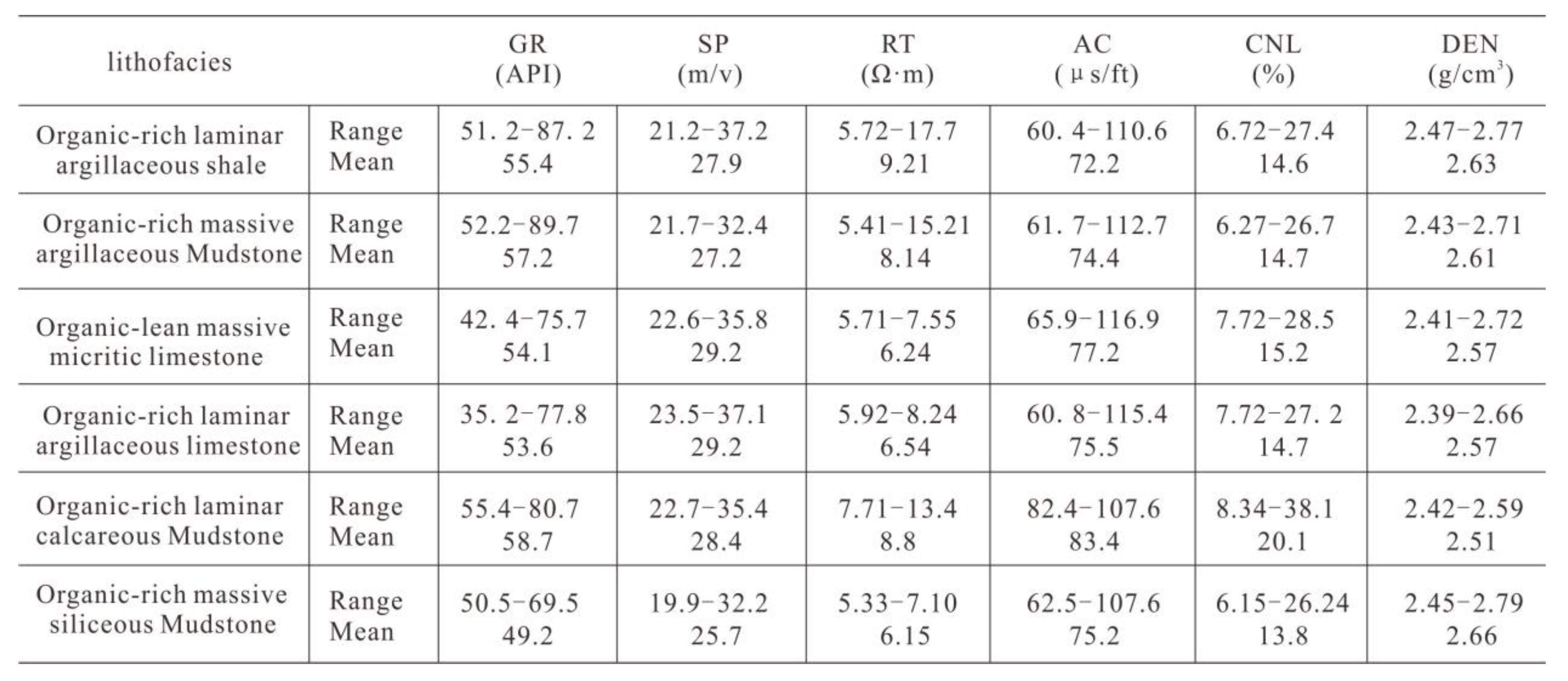
Based on the observation and description of continuous cores from single wells, we identified 12 lithofacies types, including six major ones, for the shale strata in the X member of the western slope zone in the western part of the Liaohe (Figure 4 and Figure 5). the shale lithofacies type was determined based on “organic matter abundance, rock type and mineral composition”, and based on this, a comparative analysis of the lithofacies logging effect was conducted to select a machine learning algorithm suitable for the regional characteristics, and then to explore the application of this method in the prediction of the lithofacies distribution of the whole well section. This will provide a basis for the subsequent selection of shale oil deserts.

According to the logging curve characteristics of different types of shale lithofacies, most of the data of shale lithofacies types in the study are seriously overlapped, and the conventional linear analysis method cannot meet the requirements of division, so it is necessary to carry out the study of shale lithofacies division based on machine learning (Figure 6).

3.2. Analysis of Recognition Effect of Different Algorithms for Supervised Learning

This article analyzes the recognition effect of different algorithms for supervised learning. Supervised learning algorithms target specific manually marked targets for classification or regression and have strong interpretability due to human supervision. In shale lithofacies identification, the curve characteristics of different types may overlap, resulting in different applicable effects for commonly used algorithms. Therefore, this study examines the effectiveness of different algorithms in the identification process.

This paper utilizes random sub-sampling to perform cross-validation on rock identification data. The data are divided into two groups, with 75% of the data used for training and 25% for verification. The training subset is optimized during the classification process and then applied to the independent verification data set and all data records. By dividing the data into two subsets and considering both training and verification, the model is able to provide information for external prediction of invisible data and improve accuracy in machine learning.

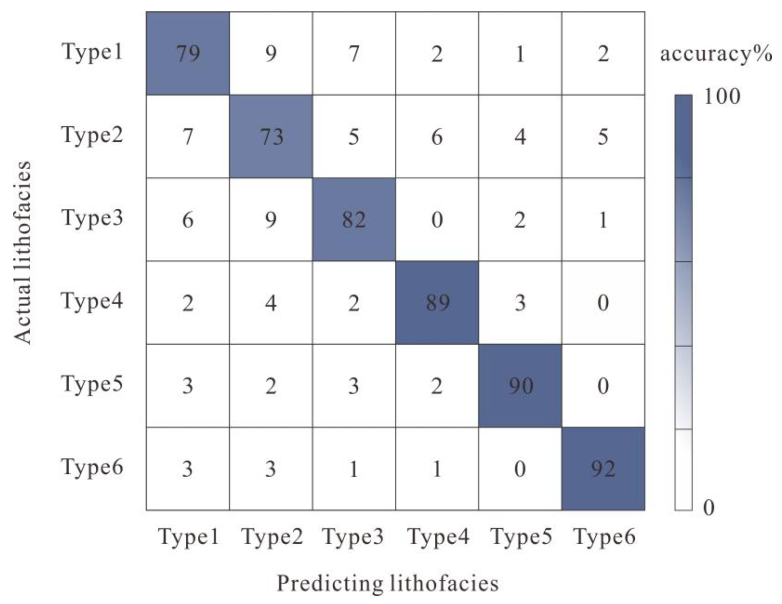
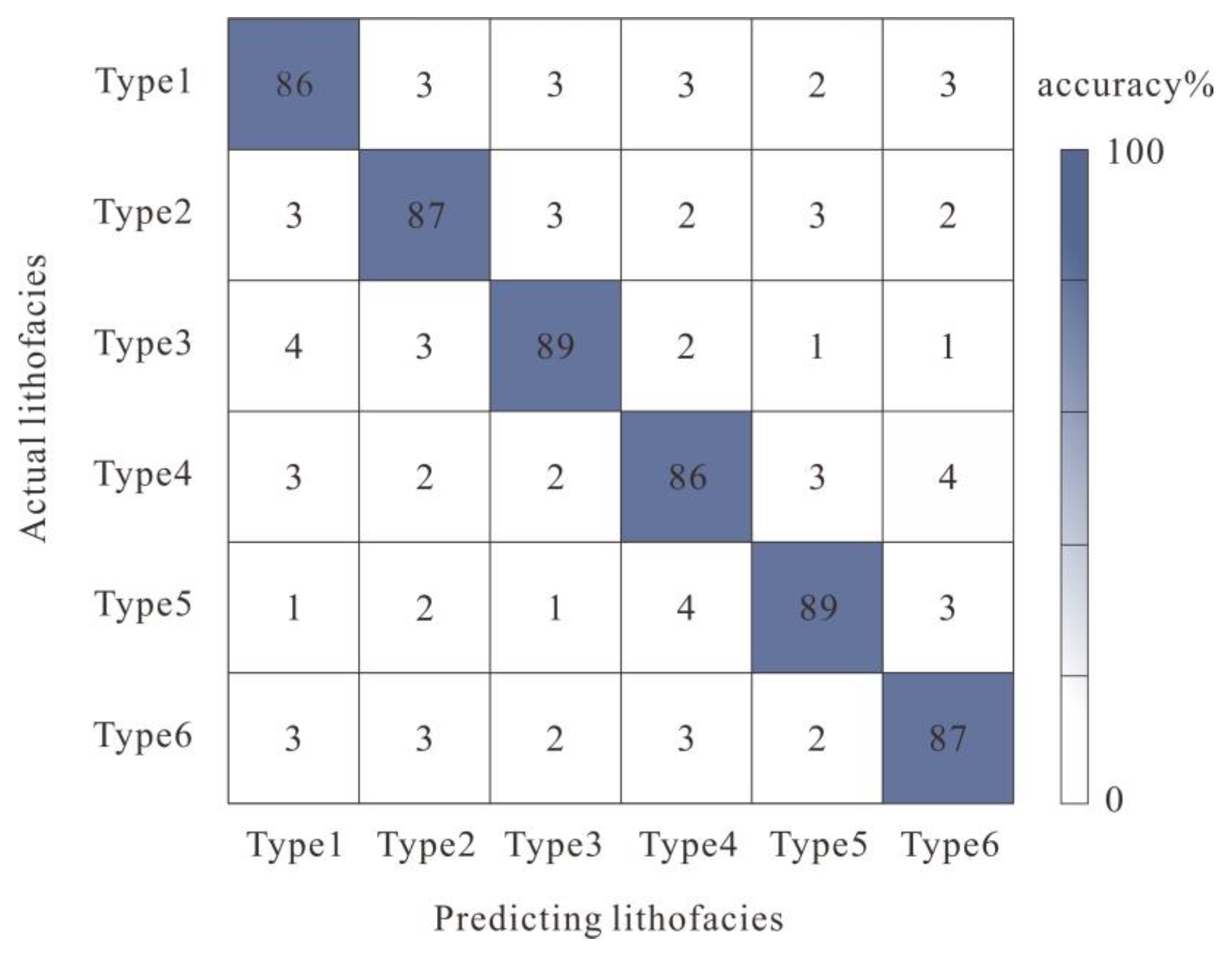
In academic research, the accuracy of an algorithm can be evaluated by using a confusion matrix diagram. This tool helps to visually measure and predict how well the algorithm matches discrete lithofacies intervals. The correct classification rate index is used to indicate the percentage of correctly estimated data points from the total number of evaluated data points. This index is useful for assessing the accuracy of distinguishing each lithofacies by each model.

3.2.1. BPANN Algorithm Recognition Effect

The BPANN algorithm is important in the field of artificial intelligence. According to the confusion matrix diagram (Figure 7) of the BP neural grid algorithm for the discrimination and analysis of lithology, the average accuracy rate of the BPANN algorithm is 84%, and the overall accuracy rate can meet the needs of shale facies identification. In particular, the identification accuracy rate of limestone and mudstone facies is relatively high, and the overall accuracy rate can reach 89.5%. However, the recognition accuracy of shale facies with two different structural features is poor, and both values are below 75%.

3.2.2. RF Algorithm Recognition Effect

The RF algorithm is a supervised machine learning algorithm that uses multiple trees to train and predict sample lithology data as a classifier algorithm. The parameters of the model were optimized using a 5-fold cross-validation method due to the limited number of samples. This approach involved randomly dividing the training set into five parts, with four parts used for training and one for verification. After parameter optimization, the optimal number of iterations was found to be 120, the maximum tree depth was set to 10, and the minimum sample number of leaf nodes was set to 1.

According to the confusion matrix diagram (Figure 8) of the RF algorithm for lithology discrimination and analysis, the RF algorithm has achieved good accuracy with an overall accuracy of about 84.1%. In particular, the recognition degree of laminated limestone mudstone and massive silty mudstone is good, with an accuracy of more than 92%. However, the recognition accuracy of the two types of shale facies is relatively low at less than 80%. Therefore, for the recognition and classification of shale facies, the RF algorithm accuracy is lacking.

3.2.3. GBDT Algorithm Recognition Effect

The model parameters of the GBDT algorithm are optimized; the number of decision trees in this study is 29, and the maximum depth of decision trees is 9 through grid search cross-validation. According to the confusion matrix diagram (Figure 9) of the GBDT for lithology discrimination analysis, the identification accuracy of the GBDT algorithm for shale lithofacies is 90.6%, and that for various lithofacies types is 89%, 91%, 89%, 90%, 92%, and 93%. The overall recognition effect is relatively good, and the fine-logging curve features between shale facies types 1 and 2 can be extracted and analyzed. Therefore, the GBDT algorithm is suitable for identifying shale facies, and its accuracy is sufficient to provide reliable prediction results.

3.2.4. KNN Algorithm Recognition Effect

This study examines the recognition effect of the KNN algorithm on lithofacies identification, focusing on the distance between points and the selection of K value. Euclidean distance is used for the distance metric, and after parameter optimization, the final value of K is determined to be 15. The confusion matrix diagram (Figure 10) shows that the KNN algorithm achieves an accuracy of 84.4% in identifying shale lithofacies and an accuracy of 84%, 83%, 83%, 82%, 85%, and 85% in identifying various lithofacies types. Overall, the recognition effect of the KNN algorithm is relatively good.

3.2.5. SVM Algorithm Recognition Effect

During the process of optimizing the support vector machine model, two hyperparameters need to be adjusted: the kernel function and another parameter that varies depending on the chosen kernel function. These two parts are not parallel. To optimize these hyperparameters, the grid search algorithm is utilized. The SVM model with the best performance in this learning process is the SVM-polynomial kernel with the following hyperparameters: c = 1.1, Gamma = 0.7, and d is left unspecified. The confusion matrix diagram (Figure 11) for discriminant analysis of lithofacies by the SVM algorithm shows that the accuracy of identifying shale lithofacies is 87.3%. The accuracy of identifying various lithofacies types is 86%, 87%, 89%, 86%, 89%, and 85%, respectively. Overall, the recognition effect is relatively good.

3.3. Analysis of Recognition Effect of Unsupervised Learning Algorithm

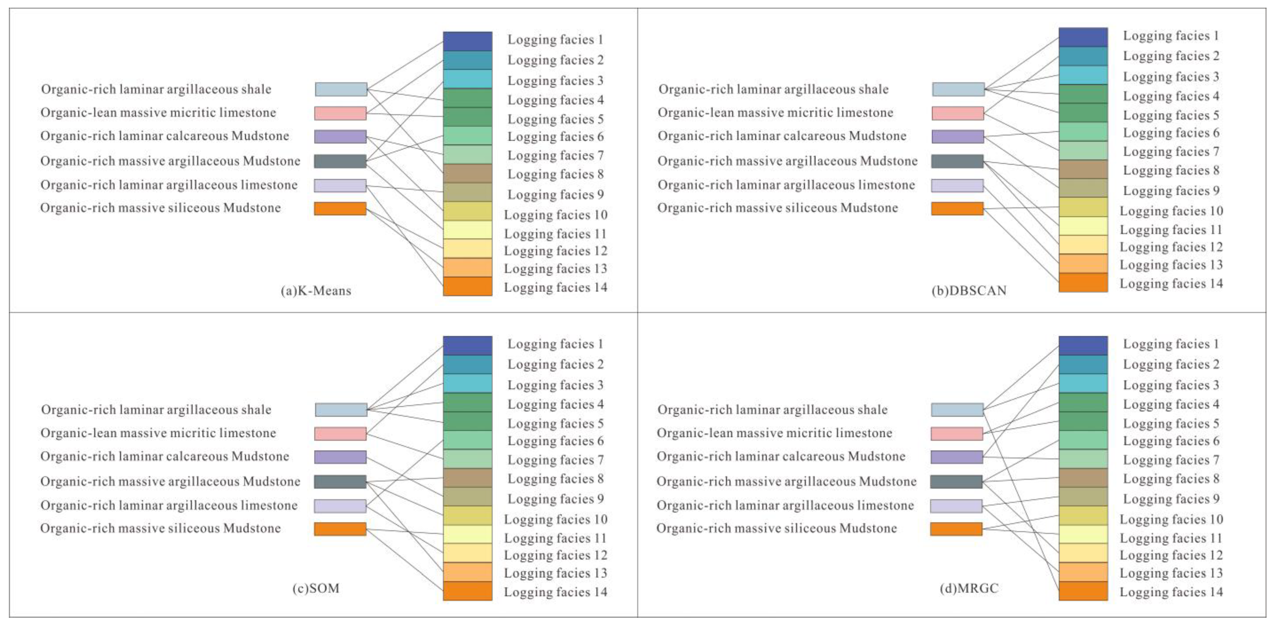
Unsupervised learning algorithms do not have a definite result because their input data are unmarked, and the sample category determined by this algorithm is unknown. This is mainly because samples need to be classified based on their similarity. In the process of identifying lithofacies, unsupervised learning algorithms first determine the number of clustered logging facies, then cluster to obtain logging facies, and then calibrate cores with coring wells to establish the corresponding relationship between logging facies and lithofacies. Finally, the logging facies are converted into lithofacies to identify lithofacies of non-coring wells and non-coring sections. To ensure accuracy in logging facies, it is recommended to have a greater number of logging facies compared to lithofacies. This helps in establishing a clear relationship between logging facies and lithofacies. As per practical experience, it is recommended to have 2–3 times more logging facies than lithofacies.

The identification of rock through logging facies is dependent on the correspondence between the two. This correspondence is established through the experience of a large number of cores and existing logging theory. Even with a small number of core samples, the cluster analysis method can still identify lithofacies. The analysis of logging facies is crucial in this method as it is converted into lithofacies. It is important to note that during this conversion process, one rock may correspond to multiple logging facies. Additionally, certain types of shale lithofacies may be relatively insensitive to single or few logging curves.

This paper comprehensively develops four unsupervised learning algorithms for shale lithofacies identification using the concept of logging facies. The identification process involves a complicated correspondence due to the different types of logging facies corresponding to different types of shale lithofacies. Organic-rich laminar argillaceous shale and organic-rich massive argillaceous mudstone correspond to multiple logging facies types due to their relatively complex types (Figure 12).

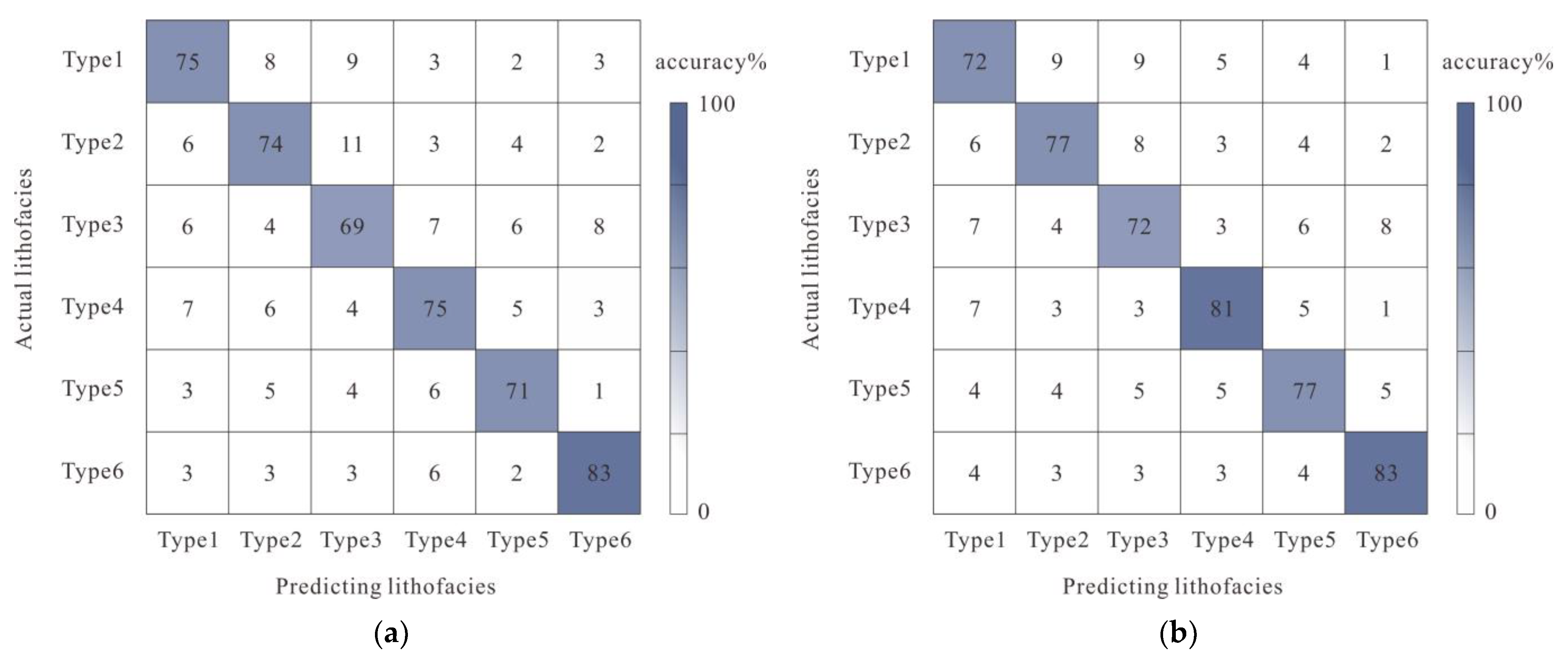
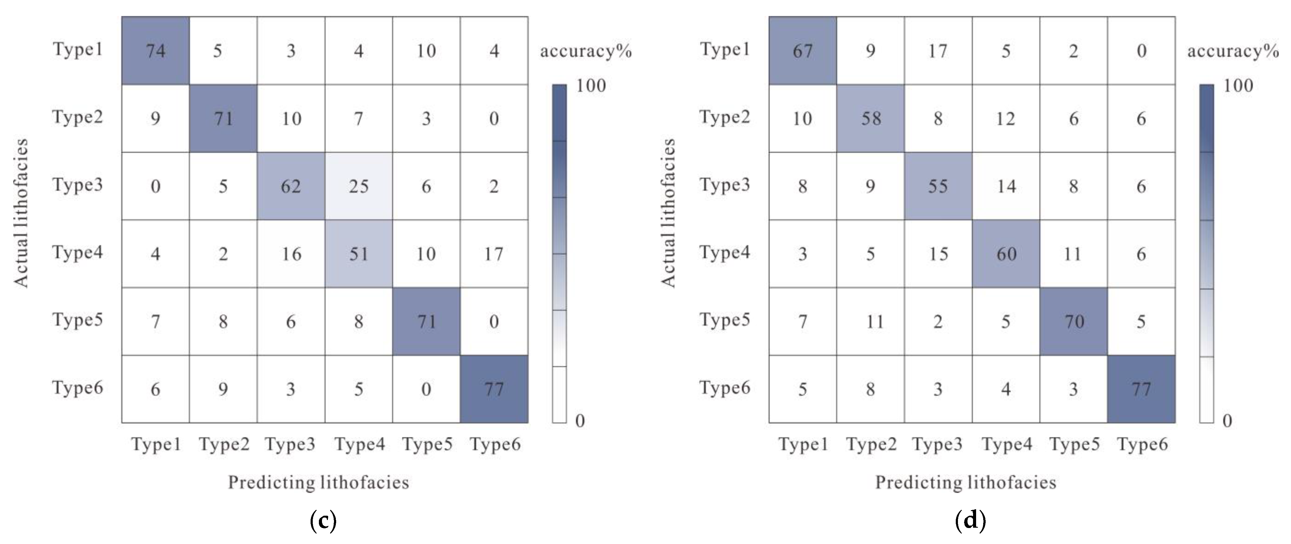
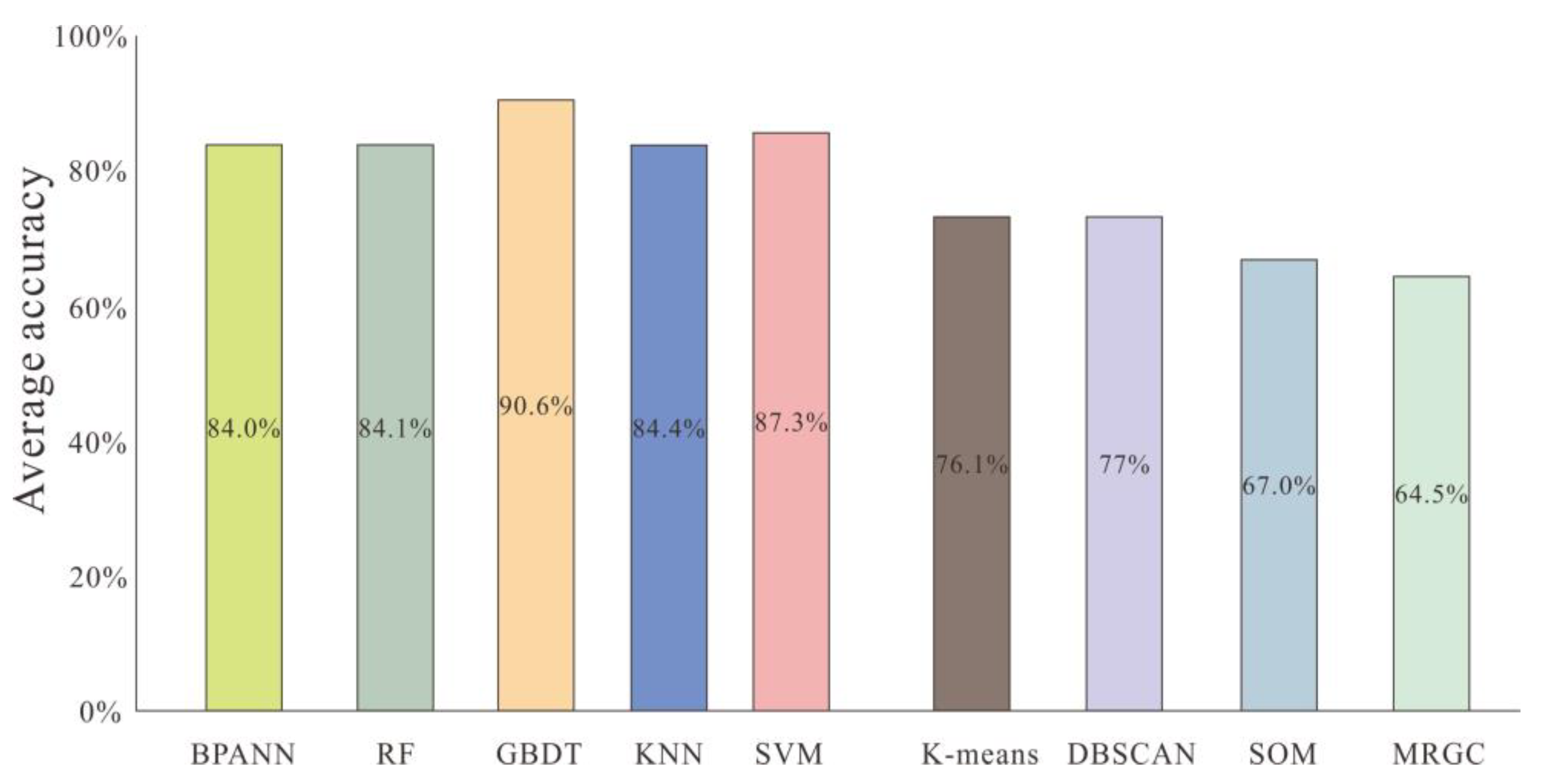
The lithofacies and logging facies of four supervised learning algorithms were compared to identify lithofacies of verification wells. The results are shown in Figure 13. The K-MEANS algorithm had an identification accuracy of about 76.1%, the DBSCAN algorithm had an accuracy of about 77%, the SOM algorithm had an accuracy of about 67%, and the MRGC algorithm had an accuracy of about 64.5%. Overall, the accuracy of shale identification results using unsupervised learning algorithms is relatively low, with the DBSCAN and K-MEANS algorithms having higher accuracy.

4. Discussion

4.1. Comparison and Comprehensive Analysis of the Results of Different Algorithms

This paper presents a comparison and comprehensive analysis of different algorithms used to identify shale lithofacies in the fourth member of the Shahejie Formation in a depression in Bohai Bay Basin. The study uses five supervised learning algorithms (BPANN, RF, GBDT, KNN, and SVM) and four unsupervised learning algorithms (K-means, DBSCAN, SOM, and MRGC). The results show that the GBDT algorithm has high accuracy among the supervised learning algorithms, while the accuracy of unsupervised learning algorithms such as K-means and DBSCAN can meet the needs of shale rock identification (Figure 14).

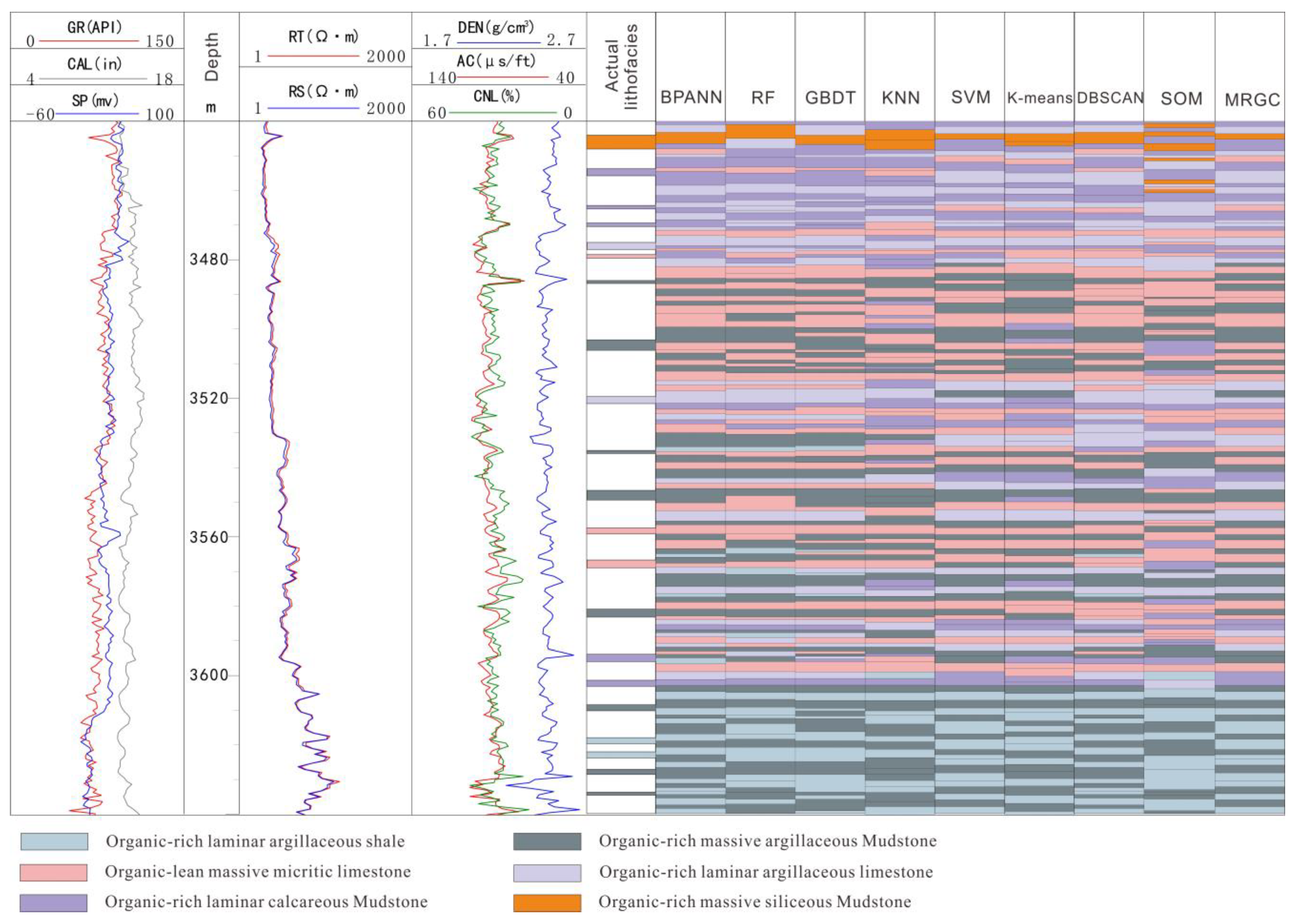
Regarding continuous prediction and evaluation of single wells, the RF, BPANN, and GBDT algorithms exhibit high accuracy. However, the GBDT algorithm has the highest accuracy, indicating its highest reliability for shale facies recognition and prediction. It can fill the gap in obtaining complete shale facies distribution characteristics due to the inability to continuously core and greatly improve the efficiency of facies recognition. Taking X well as an example, the predicted results (Figure 15) show that the vertical shale facies exhibit characteristics such as rapid type change and thin sedimentary thickness, indicating extremely strong heterogeneity. The upper part mainly consists of organic-rich laminar calcareous mudstone, and the central part mainly consists of organic-lean mass microbial limestones and organic-rich mass argillaceous mudstone. The bottom part, the main high-quality reservoir interval, mainly consists of organic-rich laminar argillaceous shale.

4.2. Summary of Advantages and Disadvantages of Different Methods in Shale Lithofacies Division

4.2.1. Advantages and Disadvantages of Supervised Learning Algorithm in Shale Identification

Among the supervised machine learning methods, including BPANN, RF, GBDT, KNN, and SVM algorithms, the key to algorithm learning lies in the typicality of learning training samples and the balance of quantity. The BPANN algorithm has a strong ability of self-adaptation. However, due to the limited basic data samples of shale lithofacies, the BPANN algorithm cannot observe the previous learning process in the black box process, which can lead to local minima and less accuracy in the identification process of shale. The random forest algorithm is known for its ability to prevent over-fitting and its high accuracy compared to other single algorithms.

However, it can experience over-fitting when the range of lithofacies type features is wide. On the other hand, the GBDT algorithm is a powerful classifier that effectively captures the nonlinear relationship between shale lithofacies and logging parameters. It has high accuracy in predicting shale lithofacies types with few samples and high class domain overlap. Additionally, it can effectively predict shale lithofacies. The KNN algorithm has a faster model training time, but its ability to divide data with overlapping or overlapping domains is relatively weak. The SVM algorithm can utilize kernel functions to map data to high-dimensional space. However, due to its slow operation process and sensitivity to missing data, it may not be the best choice for shale facies division. Currently, supervised learning is the mainstream method for classification, and it is important to consider whether the machine learning algorithm can handle the multiple superposition of data, the demand for the number of core samples, and its fault tolerance during shale lithofacies classification. The random forest algorithm and the gradient boosting decision tree algorithm have strong composite ability, making them ideal for shale lithofacies identification.

4.2.2. Advantages and Disadvantages of Unsupervised Learning in Shale Identification

Among unsupervised learning algorithms, K-MEANS is a simple and easy-to-implement algorithm. However, in identifying shale lithofacies, its clustering results are sensitive to the initial screened lithofacies characteristic values, which can lead to local optima. Furthermore, when there are many types of shale lithofacies, only spherical clusters can be found, which leads to poor results in dealing with overlapping domains. In contrast, the DBSCAN algorithm can find spatial clusters with arbitrary shapes and effectively deal with abnormal points in shale lithofacies logging response. It is less sensitive to abnormal point data, resulting in better discrimination results compared to the K-MEANS algorithm. The SOM algorithm is known for optimizing samples through neural network training, providing good stability and often yielding good results when the number of core samples is abundant. However, in the case of shale lithofacies, where the number of samples is relatively small, the classification results are limited due to the dependence on the sequence of pattern input. On the other hand, the MRGC algorithm is suitable for cases with many overlapping domains and complex logging curve characteristics, such as shale facies. It can yield better results if there are enough lithofacies classification effects.

Identifying shale lithofacies with limited sample data and overlapping data is crucial for improving unsupervised learning algorithms in shale lithofacies identification.

4.3. Prospect of Machine Learning in Shale Lithofacies Identification

The limited data of coring interval for the core type concerned are a major challenge in developing and applying machine learning algorithms for shale lithofacies classification. However, logging curve information can be used to enhance the characterization of non-coring intervals, thus improving the confidence of the machine learning algorithm’s application model. Several scholars have conducted research in this area, and based on the findings of this paper, we recommend that future research focus on exploring the following aspects to improve the accuracy and generalization of the machine learning model for shale lithofacies. To ensure accuracy, we recommend using random sub-sampling cross-validation analysis to verify the trained model with coring well data. Additionally, it is important to test the model with non-coring well data that have not been previously seen. To improve the model, consider incorporating a variety of machine learning algorithms, including the fusion of different types, to take advantage of their individual strengths. The identification and division of lithofacies in shale reservoirs is not the final step in the study. To improve the accuracy of lithofacies analysis and strengthen the connection with the classification and evaluation of shale reservoirs in later stages, it is important to incorporate parameters such as porosity, permeability, and water/oil saturation directly into machine learning. Doing so will provide supporting knowledge for identifying reservoir features and predicting distribution features in later stages.

5. Conclusions

This paper discusses the applicability of nine different machine learning algorithms in identifying shale lithofacies. The supervised learning algorithm has high accuracy, while the GBDT algorithm is a strong classifier that effectively captures the nonlinear relationship between shale lithofacies and logging parameters. It has high accuracy for predicting shale lithofacies types with few samples and high class domain overlap and can effectively predict shale lithofacies. The DBSCAN algorithm is a useful unsupervised learning method for identifying spatial clusters with arbitrary shapes and handling abnormal points in shale lithofacies logging response. It has low sensitivity to abnormal point data, making it a reliable option for achieving good discrimination results. This paper summarizes the research prospects of using machine learning to identify shale lithofacies. The main focus is on improving the prediction accuracy of lithofacies types using unsupervised learning algorithms on non-cored well data that have not been seen before. Additionally, the paper emphasizes the importance of integrating various machine learning algorithms, including the use of different types of algorithms, to leverage the advantages of each algorithm multiple times. By integrating various parameters, we can improve the accuracy of lithofacies analysis and strengthen the connection with classification and evaluation of shale reservoirs. This will provide valuable knowledge for identifying reservoir features and predicting their distribution in the later stages.

References

1. Liu, Z.; Zhuang, Z.; Meng, Q.; Zhan, S.; Huang, K. Mechanical problems and challenges of efficient production of shale gas. J. Mech. 2017, 49, 507–516. [Google Scholar]
2. Liu, B.; Wang, H.; Fu, X.; Bai, Y.; Bai, L.; Jia, M.; He, B. Lithofacies and depositional setting of ahighly prospective lacustrine shale oil succession from the Upper Cretaceous Qing shan kou Formationin the Gulong Sag, northern Song liao Basin, northeast China. AAPG Bull. 2019, 103, 405–432. [Google Scholar] [CrossRef] [Green Version]
3. Li, J.; Wang, M.; Chen, Z.; Lu, S.; Chen, G.; Tian, S. Evaluating the total oil yield using a single routine Rock-Eval experiment on as-received shales. J. Anal. Appl. Pyrolysis 2019, 144, 104707. [Google Scholar] [CrossRef]
4. Zhang, B.; Mao, Z.; Zhang, Z.; Yuan, Y.; Chen, X.; Shi, Y.; Liu, G.; Shao, X. Black shale formation environment and its control on shale oil enrichment in Triassic Chang 7 Member, Ordos Basin, NW China. Pet. Explor. Dev. 2021, 48, 1304–1314. [Google Scholar] [CrossRef]
5. Lin, M.; Xi, K.; Cao, Y.; Liu, Q.; Zhang, Z.; Li, K. Petrographic features and diagenetic alteration in the shale strata of the Permian Lucaogou Formation, Jimusar sag, Junggar Basin. J. Pet. Sci. Eng. 2021, 203, 108684. [Google Scholar] [CrossRef]
6. Li, Q.; Lan, B.; Li, G. Element geochemical characteristics and geological significance of Wufeng—Longmaxi Formation shale in the northern margin of Central Guizhou Uplift. Geoscience 2021, 46, 3172–3188. [Google Scholar]
7. Ameen, M.S.; Hailwood, E.A. A new technology for the characterization of microfractured reservoirs (test case: Unayzah reservoir, Wudayhi field, Saudi Arabia). AAPG Bull. 2008, 92, 31–52. [Google Scholar] [CrossRef]
8. Lai, J.; Wang, G.; Wang, S.; Cao, J.; Li, M.; Pang, X.; Han, C.; Fan, X.; Yang, L.; He, Z.; et al. A review on the applications of image logs in structural analysis and sedimentary characterization. Mar. Pet. Geol. 2018, 95, 139–166. [Google Scholar] [CrossRef]
9. Zhang, J. Well logging evaluation method of shale oil reservoirs and its applications. Prog. Geophys. 2012, 27, 1154–1162. [Google Scholar]
10. Zhang, C.; Zhang, L.; Chen, J.; Luo, H.; Liu, S. Lithofacies types and discrimination of Paleogene fine-grained sedimentary rocks in the Dongying Sag, Bohai Bay Basin, China. Nat. Gas Geosci. 2017, 28, 713–723. [Google Scholar]
11. Yan, J.; He, X.; Hu, Q.; Tang, H.; Feng, C.; Geng, B. Lower Es3 in Zhanhua Sag, Jiyang Depression: A case study for lithofacies classification in lacustrine mud shale. Appl. Geophys. 2018, 15, 151–164, 361. [Google Scholar] [CrossRef]
12. Che, S. Shale lithofacies identification and classification by using logging data: A case of Wufeng-Longmaxi Formation in Fuling gas field, Sichuan Basin. Lithol. Reserv. 2018, 30, 121–132. [Google Scholar]
13. Yang, Y.; Shi, W.; Zhang, X. Identification method of shale lithofacies by logging curve: A case study from Wufeng-Longmaxi Formation in Jiaoshiba area, SW China. Lithol. Reserv. 2021, 33, 135–146. [Google Scholar]
14. Wang, S. Reservoir characteristics and oil-bearing properties of different lithofacies of Lucaogou Formation in the piedmont belt of Bogda Mountain. Xinjiang Pet. Geol. 2020, 41, 402–413. [Google Scholar]
15. Gifford, C.M.; Agah, A. Collaborative Multi-Agent Rock Facies Classification from Wireline Well Log Data. Eng. Appl. Artif. Intell. 2010, 23, 1158–1172. [Google Scholar] [CrossRef]
16. Wang, G.; Carr, T.R.; Ju, Y.; Li, C. Identifying Organic—Rich Marcellus Shale Lithofacies by Support Vector Machine Classifier in the Appalachian Basin. Comput. Geosci. 2014, 64, 52–60. [Google Scholar] [CrossRef]
17. Al Mudhafar, W.J. Integrating Component Analysis & Classification Techniques for Comparative Prediction of Continuous & Discrete Lithofacies Distributions. In Proceedings of the Offshore Technology Conference, Houston, TX, USA, 7 May 2015. [Google Scholar]
18. Narayan, S.; Sahoo, S.D.; Kar, S.; Pal, S.K.; Kangsabanik, S. Improved reservoir characterization by means of supervised machine learning and model-based seismic impedance inversion in the Penobscot field, Scotian Basin. Energy Geosci. 2023, 100180. [Google Scholar] [CrossRef]
19. Lu, G.; Zeng, L.; Dong, S.; Huang, L.; Liu, G.; Ostadhassan, M.; He, W.; Du, X.; Bao, C. Lithology identification using graph neural network in continental shale oil reservoirs: A case study in Mahu Sag, Junggar Basin, Western China. Mar. Pet. Geol. 2023, 150, 106168. [Google Scholar] [CrossRef]
20. Cui, Q.; Yang, H.; Li, X.; Lu, Y. Identification of lithofacies and prediction of mineral composition in shales—A case study of the Shahejie Formation in the Bozhong Sag. Unconv. Resour. 2022, 2, 72–84. [Google Scholar] [CrossRef]
21. Ren, Q.; Zhang, H.; Zhang, D.; Zhao, X. Lithology identification using principal component analysis and particle swarm optimization fuzzy decision tree. J. Pet. Sci. Eng. 2023, 220, 111233. [Google Scholar] [CrossRef]
22. Ramos, M.M.; Bijani, R.; Santos, F.V.; Lupinacci, W.M.; Freire, A.F.M. Analysis of alternative strategies applied to Naïve-Bayes classifier into the recognition of electrofacies: Application in well-log data at Recôncavo Basin, North-East Brazil. Geoenergy Sci. Eng. 2023, 227, 211889. [Google Scholar] [CrossRef]
23. Zhao, Z.; Su, S.; Shan, X.; Li, X.; Zhang, J.; Jing, C.; Ren, H.; Li, A.; Yang, Q.; Xing, J. Lithofacies identification of shale reservoirs using a tree augmented Bayesian network: A case study of the lower Silurian Longmaxi formation in the changning block, South Sichuan basin, China. Geoenergy Sci. Eng. 2023, 221, 211385. [Google Scholar] [CrossRef]
24. Antariksa, G.; Muammar, R.; Lee, J. Performance evaluation of machine learning-based classification with rock-physics analysis of geological lithofacies in Tarakan Basin, Indonesia. J. Pet. Sci. Eng. 2022, 208, 109250. [Google Scholar] [CrossRef]
25. Wang, P.; Chen, X.; Wang, B.; Li, J.; Dai, H. An improved method for lithology identification based on a hidden Markov model and random forests. Geophysics 2020, 85, IM27–IM36. [Google Scholar] [CrossRef]
26. Feng, R. Improving uncertainty analysis in well log classification by machine learning with a scaling algorithm. J. Pet. Sci. Eng. 2021, 196, 107995. [Google Scholar] [CrossRef]
27. Liu, M.; Hu, S.; Zhang, J.; Zou, Y. Methods for identifying complex lithologies from log data based on machine learning. Unconv. Resour. 2023, 3, 20–29. [Google Scholar] [CrossRef]
28. Ali, N.; Chen, J.; Fu, X.; Hussain, W.; Ali, M.; Iqbal, S.M.; Anees, A.; Hussain, M.; Rashid, M.; Thanh, H.V. Classification of reservoir quality using unsupervised machine learning and cluster analysis: Example from Kadanwari gas field, SE Pakistan. Geosyst. Geoenviron. 2023, 2, 100123. [Google Scholar] [CrossRef]
29. Zhao, F.; Yang, Y.; Kang, J.; Li, X. CE-SGAN: Classification enhancement semi-supervised generative adversarial network for lithology identification. Geoenergy Sci. Eng. 2023, 223, 211562. [Google Scholar] [CrossRef]
30. Abbas, L.K.; Mahdi, T.A. Reservoir units of Mishrif Formation in Majnoon oil field, southern Iraq. Iraqi J. Sci. 2019, 60, 2656–2663. Available online: http://scbaghdad.edu.iq/eijs/index.php/eijs/article/view/1252 (accessed on 5 June 2023). [CrossRef]
31. Al-Mudhafar, W.J.; Al Lawe, E.M.; Noshi, C.I. Clustering analysis for improved characterization of carbonate reservoirs in a southern Iraqi oil field. In Proceedings of the Offshore Technology Conference, Houston, TX, USA, 6–9 May 2019. [Google Scholar] [CrossRef]
32. Zheng, W.; Tian, F.; Di, Q.; Xin, W.; Cheng, F.; Shan, X. Electrofacies classification of deeply buried carbonate strata using machine learning methods: A case study on ordovician paleokarst reservoirs in Tarim Basin. Mar. Petrol. Geol. 2021, 123, 104720. [Google Scholar] [CrossRef]
33. Zhou, J.; Bai, H.; Cui, J.; Zhang, W.; Liang, H.; Wang, J.; Yu, Y.; He, W. Application of BP neural network model based on electromagnetic parameters in shale gas reservoir prediction. Geophys. Geochem. Calc. Technol. 2020, 42, 76–83. [Google Scholar]
34. Yuan, Y.; Tan, D.; Yu, S.; Li, Y.; Han, B. A Prediction model for shale gas organic carbon content based on improved BP neural network using Bayesian regularization. Geol. Explor. 2019, 55, 1082–1091. [Google Scholar]
35. Sun, Y.; Lyu, S.; Wang, X.; Tang, Y. K-nearest neighbor algorithm based on learning structure. Comput. Sci. 2007, 34, 184–186. [Google Scholar]
36. Sang, Y. Research on Classification Algorithm Based on K-Nearest Neighbor; Chongqing University: Chongqing, China, 2009. [Google Scholar]
37. Zhou, S.; Fu, L.; Liang, B. Clustering analysis of Ancient Celad on based on SOM neural network. Sci. China E 2008, 38, 1089–1096. [Google Scholar]
38. Fu, X.; Zhang, A. Feature selection of SOM based intrusion detection algorithm. J. Huazhong Univ. Sci. Technol. Nat. Sci. Ed. 2007, 35, 5–7. [Google Scholar]
39. Kohonen, T. Self-organized formation of topologically correct featuremaps. Biol. Cybern. 1982, 43, 59–69. [Google Scholar] [CrossRef]
40. Chang, H.C.; Kopaska-Merkel, D.C.; Chen, H.C. Identification of lithofacies using Kohonen self-organizing maps. Comput. Geosci. 2002, 28, 223–229. [Google Scholar] [CrossRef]
41. Zhang, M. Study on Multi-Level Self-Organization Automatic Classification Method for Stratigraphy Lithology; Yangtze University: Wuhan, China, 2018. [Google Scholar]
42. Finthan, B.; Mamman, Y.D. The lithofacies and depositional paleoenvironment of the Bima Sandstone in Girei and Environs, Yola Arm, Upper Benue Trough, Northeastern Nigeria. J. Afr. Earth Sci. 2020, 169, 103863. [Google Scholar] [CrossRef]
43. Borka, S. Markov chains and entropy tests in genetic-based lithofacies analysis of deep-water clastic depositional systems. Open Geosci. 2016, 8, 45–51. [Google Scholar] [CrossRef] [Green Version]
44. Könitzer, S.F.; Davies, S.J.; Stephenson, M.H. Depositional controls on mudstone lithofacies in a basinal setting: Implications for the delivery of sedimentary organic matter. J. Sediment. Res. 2014, 84, 198–214. [Google Scholar] [CrossRef]
45. Nie, Y.; Xie, Q.; Zhu, X.; Zhang, M. The sedimentary mechanism and research prospect of fine grain sediments based on lithofacies characterization. Fault-Block Oil Gas Field 2021, 28, 305–310. [Google Scholar]
46. Lu, S.; Li, J.; Zhang, P.; Xue, H.; Wang, G.; Zhang, J.; Liu, H.; Li, Z. Classification of microscopic pore-throats and the grading evaluation on shale oil reservoirs. Pet. Explor. Dev. 2018, 45, 452–460. [Google Scholar] [CrossRef]
47. Liu, Q.; Zeng, X.; Wang, X. Lithofacies of mudstone and shale deposits of the Es3z-Es4s Formation in Dongying Sag and their depositional environment. Mar. Geol. Quat. Geol. 2017, 37, 147–156. [Google Scholar]
48. Liu, S.; Cao, Y.; Liang, C. Lithologic characteristics and sedimentary environment of fine-grained sedimentary rocks of the Paleogene in Dongying Sag, Bohai Bay Basin. J. Palaeogeogr. 2019, 21, 479–489. [Google Scholar]
49. Deng, Y.; Chen, S.; Pu, X.; Yan, J.; Chen, J. Formation mechanism and environmental evolution of fine-grained sedimentary rocks from the second member of Kongdian Formation in the Cangdong Sag, Bohai Bay Basin. Oil Gas Geol. 2020, 41, 811–823. [Google Scholar]
50. Zhou, L.; Han, G.; Ma, J.; Chen, C.; Yang, F.; Zhang, L.; Zhou, K. Palaeoenvironment characteristics and sedimentary model of the Lower submember of member 1 of Shahejie Formation in the southwestern margin of Qikou Sag. Acta Pet. Sin. 2020, 41, 903–917. [Google Scholar]
51. Williams, H.; Turner, F.J.; Gilbert, C.M. Petrography: An Introduction to the Study of Rocks in Thin Section, 2nd ed.; W. H. Freeman and Company: San Francisco, CA, USA, 1982. [Google Scholar]
52. Folk, R.L. Petrology of Sedimentary Rocks; Hemphill Publishing Company: Austin, TX, USA, 1980. [Google Scholar]
53. Schieber, J. Early diagenetic silica deposition in algal cysts and spores: A source of sand in black shales? J. Sediment. Res. 1996, 66, 175–183. [Google Scholar]
Figure 1. Schematic of a typical neuron model.
Processes 11 02042 g001
Figure 2. Network structure diagram of the BP neural network model.
Processes 11 02042 g002
Figure 3. Block diagram of the implementation of the GBDT model.
Processes 11 02042 g003
Figure 4. Mineral composition distribution of shale in Formation A of a depression in Bohaiwang Basin.
Processes 11 02042 g004
Figure 5. Characteristics of lithofacies type development in Formation A of a depression in Bohaiwang Basin.
Processes 11 02042 g005
Figure 6. Logging curve characteristics of typical shale lithofacies types.
Processes 11 02042 g006
Figure 7. Confusion matrix diagram of BPANN algorithm for the discrimination and analysis of shale facies.
Processes 11 02042 g007
Figure 8. Confusion matrix diagram of RF algorithm for the discrimination and analysis of shale facies.
Processes 11 02042 g008
Figure 9. Confusion matrix diagram of GBDT algorithm for the discrimination and analysis of shale facies.
Processes 11 02042 g009
Figure 10. Confusion matrix diagram of KNN algorithm for the discrimination and analysis of shale facies.
Processes 11 02042 g010
Figure 11. Confusion matrix diagram of SVM algorithm for the discrimination and analysis of shale facies.
Processes 11 02042 g011
Figure 12. Correspondence between shale lithofacies and logging facies.
Processes 11 02042 g012
Figure 13. Confusion matrix of unsupervised learning algorithm. (a) Confusion matrix diagram of K-means algorithm for the discrimination and analysis of shale facies. (b) Confusion matrix diagram of DBSCAN algorithm for the discrimination and analysis of shale facies. (c) Confusion matrix diagram of SOM algorithm for the discrimination and analysis of shale facies. (d) Confusion matrix diagram of MRGC algorithm for the discrimination and analysis of shale facies.
Processes 11 02042 g013aProcesses 11 02042 g013b
Figure 14. Accuracy histogram of different algorithms.
Processes 11 02042 g014
Figure 15. Various machine learning algorithms for the untrained number set X well identify synthetic lithofacies histogram.
Processes 11 02042 g015
Disclaimer/Publisher’s Note: The statements, opinions and data contained in all publications are solely those of the individual author(s) and contributor(s) and not of MDPI and/or the editor(s). MDPI and/or the editor(s) disclaim responsibility for any injury to people or property resulting from any ideas, methods, instructions or products referred to in the content.