Article

CFD Validation of Moment Balancing Method on Drag-Dominant Tidal Turbines (DDTTs)

School of Mechanical and Aerospace Engineering (MAE), Nanyang Technological University, 50 Nanyang Avenue, Singapore 639798, Singapore
*
Author to whom correspondence should be addressed.
Processes 2023, 11(7), 1895; https://doi.org/10.3390/pr11071895
Submission received: 29 May 2023 / Revised: 17 June 2023 / Accepted: 21 June 2023 / Published: 23 June 2023
(This article belongs to the Special Issue Multiscale Modeling and Numerical Simulation of Multiphase Flow)

Abstract

:
Current performance analysis processes for drag-dominant tidal turbines are unsuitable as disk actuator theory lacks support for varying swept blockage area, bypass flow downstream interaction, and parasitic rotor drag, whereas blade element momentum theory is computably effective for three-blade lift-dominated aerofoil. This study proposes a novel technique to calculate the optimal turbine tip speed ratio (TSR) with a cost-effective and user-friendly moment balancing algorithm. A reliable dynamic TSR matrix was developed with varying rotational speeds and fluid velocities, unlike previous works simulated at a fixed fluid velocity. Thrust and idle moments are introduced as functions of inlet fluid velocity and rotational speed, respectively. The quadratic relationships are verified through regression analysis, and net moment equations are established. Rotational speed was a reliable predictor for Pinwheel’s idle moment, while inlet velocity was a reliable predictor for thrust moment for both models. The optimal (Cp, TSR) values for Pinwheel and Savonius turbines were (0.223, 2.37) and (0.63, 0.29), respectively, within an acceptable error range for experimental validation. This study aims to improve prevailing industry practices by enhancing an engineer’s understanding of optimal blade design by adjusting the rotor speed to suit the inlet flow case compared to ‘trial and error’ with cost-intensive simulations.

1. Introduction

Tidal energy holds significant potential for growth as a dependable source of energy worldwide to provide economic relief for communities near coastlines or tidal channels generating well above 130,000 terawatt-hours of electricity per year [1,2,3,4,5]. The energy generated could power residential, commercial, and tourism sectors through smart grid infrastructure. Ocean energy technologies, such as tidal and wave energy, have the potential to meet 10% of the EU’s power demand by 2050 [6].
Drag-dominated tidal turbines (DDTTs) feature simpler geometries and operate at lower flow velocities, making them well-suited for deployment in slow water currents. DDTTs consist of axial or crossflow turbines where the axis of rotation is horizontal or vertical to the inflow direction, respectively. In this paper, the DDTTs of Pinwheel, as a horizontal axis turbine, and Savonius, as a vertical axis turbine, were studied as two typical examples. In the past numerical simulation process, [7] applied the blade element momentum (BEM) theory to optimize the design of a small horizontal axis wind turbine for low wind speed areas through Q-blade software and a MATLAB script. The authors of [8] experimentally evaluated the performances of Pinwheel rotors with different cutting styles in a wind tunnel, finding that the tip speed ratio (TSR or λ) decreased as the number of blades increased and that Cp was maximum for the four-bladed rotor. The authors of [9] compared the performances of eleven different configurations of Pinwheel wind turbines to discover an optimal TSR of 5.5, with a cut-in speed of 1.65 m/s and a cut-off speed of 12.5 m/s, through computational fluid dynamics (CFD) simulation and Weibull distribution.
In the exploration of blade optimization, [10] found that a two-bladed single-stage Savonius tidal turbine achieved the highest experimental power coefficient in comparison to those with three or four blades. The authors of [11,12] conducted experimental studies in a wind tunnel and validated the inverse relation between performance and the overlap ratio, i.e., the ratio of the area where the blades of the turbine overlap to the total area swept by the blades. The authors of [13,14] investigated performance improvement by a parabolic and Myring Equation-inspired blade design using two-dimensional transient simulations, whereas [15,16] analyzed a helical and humpback whale-inspired blade design, respectively, using ANSYS-CFX code.
In the exploration of the hydrodynamic system, [17] presented an experimental and computational design analysis of a direct drive-vertical axis Darrieus hydrokinetic turbine. Through 2D simulations, their results showed improved energy extraction compared to single rotor designs, good torque smoothing, flow velocity reduction, and lift generation. Future work includes conducting 3D simulations to analyze vorticity flow patterns, utilizing large-eddy simulations for recirculation regions, and performing an analysis of multi-blade profiles and lag angles for design optimization. The study by [2] aimed to develop a simplified analytical method for calculating the backwater and blockage effects of hydrokinetic turbines in inland water systems. This was achieved by using CFD models and a validated multiphase model. They provided a simplified tool for first-order analysis of backwater in the deployment of inland turbine systems, which incorporated flow velocity and thrust coefficient. The tool was validated through scaled model experiments. The authors of [18] investigated diffuser-augmented tidal turbines and discovered an effective reduction in blade tip losses using a diffuser. Furthermore, the practical evaluation of this turbine conducted offshore at Daishan Island confirmed slightly higher energy efficiency compared to the experimental model, thus validating its application potential. In their work, [19] considered the optimized array layout of a hydrokinetic turbine farm in canals, involving rotor geometry, turbine spacing, and array spacing while managing backwater effects. This approach considered rotor fluid dynamics losses and overcame the limitations of actuator disc models.
This research presents a novel optimization strategy for enhancing the blade design and power generation of DDTTs by generating a preliminary result to enhance the engineer’s understanding before choosing from a wide range of available computational techniques. The strengths of this study are as follows:
  • Dynamic TSR matrix: Varying TSR by adjusting turbine rotational speed with inflow velocity for realistic conditions with a relatively simple experimental design [20,21].
  • Net moment analysis: Balancing equation derived from the sum of idle and thrust moments, aiding TSR calculation with 15.3% and 10.0% error rate (CFD model).
  • Optimal power generation: Determining power coefficient and operating conditions based on the torque–power relationship with experimental and numerical validation.
  • Robust power coefficient finder: Zero net moment identifies optimal TSR, applicable to turbines of any shape or orientation.
  • Time and cost savings: Moment parameter collection using steady and K-ε turbulence model, accessible on a standard laptop for 3D CFD models. Fast convergence saves time.

2. Methodology

2.1. Channel Parametric Study

In this work, the commercial software Star-CCM+ was utilized for the analysis of CFD models. The geometries of the Pinwheel and Savonius turbines were developed using SolidWorks and subsequently imported into the Star-CCM+ platform. The fluid domain was created in three dimensions (3D) and divided into a stationary region and a rotating domain, which, respectively, housed the Pinwheel and Savonius turbine [17]. For further investigation, Figure 1 and Figure 2 depict the top view and 3D isometric view of the computational flow domain, respectively.
To ensure accurate analysis results, the dimensions of the inlet, outlet, and surrounding walls of the stationary region were adjusted to facilitate the complete development of upstream and downstream flow without exerting any influence on the analysis. Both the inlet and outlet boundaries were positioned upstream and downstream from the centroid of the turbine system. The side, top, and bottom walls were assigned a symmetric boundary condition. In all flow simulations, seawater was considered as the working fluid. It is worth noting that the flow domain for the Savonius turbine was designed with a longer downstream length of 12D (rotor diameter), whereas the Pinwheel turbine had a downstream length of 9D. This design choice was made to ensure the attainment of a fully extended vortex for the Savonius turbine, as its wake decay length is longer than that of the Pinwheel turbine [22,23,24,25,26].
The domains’ actual scale was determined through a parametric study that aimed to equalize the blockage ratio of both models. The blockage ratio refers to the area occupied by the blades in relation to the turbine inlet area, while the aspect ratio represents the ratio of a turbine blade’s length to the rotor’s radius. An experimental investigation and numerical simulations were conducted by [27] to identify the optimal performance characteristics of a miniature Savonius turbine operating in a water channel with a low in-flow velocity of 0.5 m/s. Their findings revealed that a TSR (tip speed ratio) of 0.7 yielded the highest maximum power coefficient (Cp) value of 0.23. The selection of a 2 mm sheet thickness was based on [28]. The blockage and aspect ratio were calculated using the Savonius blade and channel area provided by [27], as outlined in Equations (1) and (2).
A s p e c t   R a t i o S a v o n i u s = C h a n n e l   W i d t h = 0.6 C h a n n e l   H e i g h t = 0.325 = 1.85
C h a n n e l   A r e a S a v o n i u s = C h a n n e l   W i d t h . C h a n n e l   H e i g h t = ( 0.6   m ) . ( 0.325   m ) = 2.36   m 2
Then, these were applied to the Pinwheel’s domain as given in Equations (3) and (4).
A s p e c t   R a t i o P i n w h e e l = C h a n n e l   W i d t h X C h a n n e l   H e i g h t Y = 1.85
C h a n n e l   A r e a P i n w h e e l = C h a n n e l   W i d t h X . C h a n n e l   H e i g h t Y = 2.36   m 2
Upon multiplying LHS and RHS of Equation (3) by Y as given in Equation (5) and substituting Y in Equation (4), the Pinwheel channel width and height were calculated as X , Y = 2.09,1.13 m.
X Y . Y Y = 2.36 Y 2 = 1.85 , t h u s , Y = 2.36 1.85 = 1.13   m
For the same aspect ratio and blockage, the significant lengths were the same, thereby affecting only the fluid velocity, which influenced the Reynolds number (Re) of the flow field [29]. The scales of the two models are tabulated in Table 1, along with the minimum and maximum Reynolds numbers observed at different flow speeds. The design of the channel blockage is illustrated in Figure 3.

2.2. Mesh Overview

The convergence rate and grid independence of results significantly influenced the computational mesh’s effectiveness [30,31,32], as established previously. In this study, we employed a combination of edge and face sizing techniques to determine the cell sizes of the mesh. For Pinwheel, an unstructured tetrahedral meshing scheme was used, while for Savonius, a polyhedral meshing scheme was employed. This approach is applicable to both stationary and rotating scenarios. We selected this methodology based on the advantages of unstructured grids, which allow for the efficient discretization of complex geometries while minimizing the need for user intervention [33,34,35]. Figure 4 provides an overview of the volume mesh, while Figure 5 shows cross-sectional views.
For the Savonius and Pinwheel simulations, the fluid temperature is assumed to be at the default values of 25 °C and 20 °C, respectively, with seawater densities of 997.56 kg/m3 and 1025 kg/m3, respectively. Both models utilized a K-ε turbulence steady-state segregated solver, with the convergence criterion set to residuals of magnitude 10−3. The fluid properties and flow models are summarized in Table 2. This consistent choice aided in comparing the Cp-TSR performance curves of the two models.
Figure 6 illustrates the variation of grid elements and the corresponding power coefficient of the two turbines for a steady-state model. For the Pinwheel turbine, a grid number of 2,080,945 cells was selected based on a fluid velocity of 0.9 m/s, rotational velocity of 7.5 rad/s, and TSR of 2.5. For the Savonius turbine, a grid number of 1,069,955 cells was selected based on a fluid velocity of 0.5 m/s, rotational velocity of 6 rad/s, and TSR of 0.7.
Figure 7 depicts the cross-sectional mesh view of the prism layer mesh applied to the surface of the two hydrofoil blades. To maintain consistency, three prism layers were utilized, with the first prism thickness set at 0.005 m and a stretching ratio of 1.2. This approach ensured the inclusion of the boundary layer in all mesh simulations, consequently reducing variability. For the blade surface, a relative target cell size of 0.2 m was selected, and the relative minimum cell size was established at 0.005 m. Given the presence of turbulent flow in the trailing edge of the hydrofoil, it necessitated a high-quality mesh.

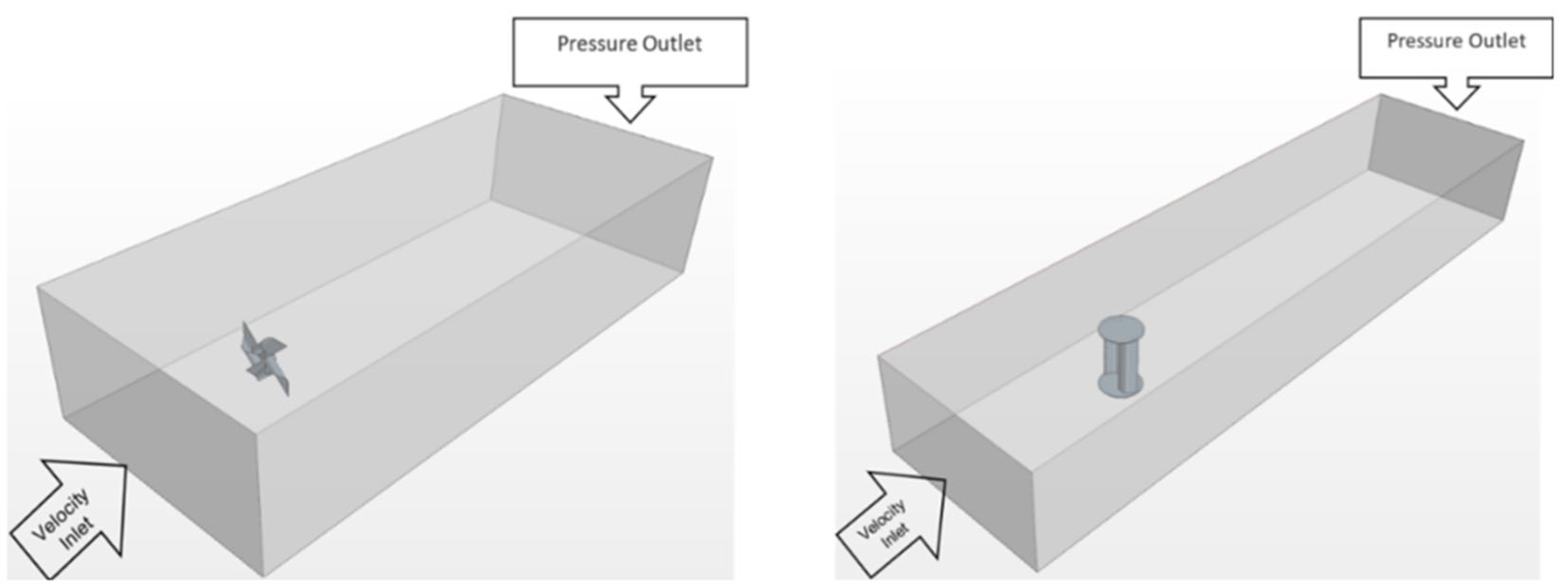
2.3. Boundary Conditions with Dynamic TSR Matrix

The two varying independent variables in this study, i.e., U 1 and ω comprise a dynamic TSR matrix using Equation (6) summarized for both turbines as Table 3 and Table 4. This method can provide a series TSR range to find the turbine’s optimal TSR by the Cp -TSR curve. The outlet pressure is set to 0 for all cases.
T S R = ω R U 1

2.4. Derivation of Characteristic Equation

Moment analysis of a single turbine configuration has been investigated in either horizontal or vertical axis cases. This study introduces two new moment definitions, the idle and thrust moments, derived mathematically from previous literature equations with respect to BCs, i.e., the rotational velocity ω and fluid velocity U 1 . The aim is to establish an equilibrium state and describe its moment balancing equation to determine the optimal power coefficient Cp,opt. Prior research utilized a fixed inlet flow speed scheme; however, this study employs a dynamic TSR matrix for the simulations.

2.4.1. Net Moment Balancing Equation

The authors of [36] studied the performance dependence of VAWTs on the moment of inertia in an unsteady wind tunnel and proposed Equation (7) with the net angular momentum Δ L as a sum of torque of wind turbine τ w , brake τ B and load τ L . The authors of [37] proposed Equation (8) for calculating the net torque on a turbine under a set optimal rotational speed operation as the motor generates a counterbalancing torque on the turbine rotor under fluid loading.
Δ L = I d w d t = τ w τ B τ L
J θ ¨ = τ R o t o r D θ ˙ τ M o t o r
The net moment when the turbine is stationary, but the fluid motion exerts load to rotate the turbine, is defined as the thrust moment, M T h r u s t ( U 1 , 0 ) , governed by the thrust coefficient C T and fluid velocity U 1 . Idle moment, M I d l e ( 0 , ω ) , is defined as when the turbine is rotating at constant speed in still water; hence, a load is exerted on the turbine. It is governed by the viscosity and centrifugal force of the fluid. Applying the principle of conservation of angular momentum and assuming steady operation in Equation (7), the sum of the external moments ( Σ τ ) is zero as derived in Equation (9) or the form of moment balancing equation in Equation (10):
Σ τ = Δ L = τ w τ L + τ B = 0
M n e t , o p t U 1 , ω = M T h r u s t U 1 , 0 + M I d l e 0 , ω = 0
where the thrust moment is the torque generated by the wind turbine, i.e., M T h r u s t = τ w , and the idle moment is equal to the sum of the load torque and the braking torque, i.e., M I d l e = τ L + τ B . In the case of the horizontal axis Pinwheel turbine, the simulation result finds that the braking torque τ B is zero, thus noted as M I d l e * .
In addition, from Equation (7), assuming steady operation and negating damping factor D , it is found that the torque produced by the motor, i.e., τ M o t o r = M I d l e counterbalances the torque experienced by the rotor blades, i.e., τ R o t o r = M T h r u s t during steady operation in the tank. This indicates that the optimal power performance is achieved when M n e t , o p t is zero, i.e., the neutral point, where the thrust and idle moment are equally offset. The significance of the moment balancing equation is to replace the unsteady cyclic volume force analysis with a simplified steady moment analysis. This method is useful in simulations for determining the values of U 1 and ω to achieve equilibrium. Engineers can determine the optimal power coefficient by observing their model results for the net moment approaching zero, indicating a neutral point where the idle and thrust moment are equal and can be used interchangeably to calculate the power coefficient using Equation (11).
C p , o p t = P e x t r a c t e d P i n = ω · M T h r u s t / I d l e 1 2 ρ A U 1 3

2.4.2. Thrust and Idle Moment Equation

The following mathematical derivations demonstrate the reason, in Equation (9), why thrust and idle moment are solely dependent on U 1 or ω , respectively. The classic equation for determining the moment on a rotor plate due to the thrust force applied is given in Equation (12).
M T h r u s t = F T h r u s t . l = 1 2 ρ A C T U 1 2 × l = ( ρ π D 3 C T 16 ) · U 1 2 ( P i n w h e e l ) ( ρ a b C T 2 ) · U 1 2 ( S a v o n i u s )
The RANS mean mass and momentum transport equations in the moving rotational frame (MRF) system were written as Equations (13) and (14) in integral form. The steady-state and incompressible flow during the idle moment is governed by the modified Navier–Stokes equations in the MRF [38]. These equations include additional centrifugal force terms in the momentum conservation, resulting in the derivation of Equation (14) as Equation (15). This term contributes to the source term of the relative coordinate system, allowing for the derivation of the idle moment on the actual disc through integration. In a steady state with static inflow velocity, the M I d l e is expressed as the force arm r times the sum of pressure difference and the centrifugal force’s term indicated as Equation (16). Hereby the M I d l e is linearly related to only the ω 2 .
t ρ d V + ρ ( U r U g ) d a = S u d V
t ρ U d V + ρ U ( U r U g ) d a = σ d a + f b d V + ρ ω × U d V
ρ ( U 1 t + U 1 2 U 1 ) = P + μ 2 U 1 + ρ ( ω 2 r + 2 ω U r o t a t i o n a l )
M I d l e = ( P d A + τ d A ) d r

2.4.3. Governing Equations with Turbulence Equations

STAR-CCM+ offers a Realizable K-Epsilon model known as the two-layer (RKE 2L) method. This model incorporates a new transport equation for turbulence dissipation rate, dividing the computation into two layers. It ensures that the critical coefficient of the model varies as a function of mean flow and turbulence properties rather than remaining constant [39,40,41].
In the near-wall layer, turbulence dissipation rate (ε) and turbulence viscosity (μt) are determined as functions of the distance from the wall. These near-wall values smoothly merge with the values obtained from solving the transport equations away from the wall. Throughout the fluid domain, the turbulent kinetic energy equation is solved. This explicit specification of ε and μt has been found to be as effective as the damping functions method and can produce comparable or even superior results [42].
Next, the segregated solver is applied to discretize and solve the mass and momentum integral conservation equations, which can be found in the STAR-CCM+ user manual. Equation (17) gives the calculation of μ t by combining the turbulence kinetic energy k and ε together.
μ t = ρ C μ f μ k 2 ε
where, C μ -Model coefficient, equal to 0.9 in RKE 2L, f μ -Damping coefficient, equal to 1 in RKE 2L.
The k and ε are obtained from the following transport equations Equation (17) and Equation (18), where the velocity and direction are derived along the x direction:
( ρ k ) t + ( ρ k U i ) x i = x i μ + μ t σ k k x i + f c G k + G b ρ ε Υ M + S k
( ρ ε ) t + ( ρ ε U i ) x i = x i μ + μ t σ ε ε x i + C 1 ε ε C 2 ε ρ ε 2 k + U i ε + ε k C 3 ε G b + S ε
where G k -Turbulent kinetic energy generation coefficient, G b -Turbulence dissipation rate generation coefficient, Υ M -Specific dissipation rate to turbulent kinetic energy ratio, C 1 ε , C 2 ε , C 3 ε -Model constants, equal to max ( 0.43 , S k 5 ε + S k ) ; 1.9 and 1.0, respectively, in RKE 2L, S k , S ε -User-defined source terms, σ k ,  σ ε -Turbulent Prandtl numbers, equal to 1.0 and 1.2, respectively, in RKE 2L.

3. Results and Discussion

The simulations were performed on a 64-bit Windows operating system. The details of the computing setup and the average computational time for one simulation case are summarized in Table 5 below.

3.1. Idle and Thrust Moment Relationship Quadratic with U 1 and ω

For internal validation of the simulation findings, the regression equations for the idle and thrust moment were calculated using multivariate linear regression analysis in Microsoft Excel, and the goodness of fit of the regression model was checked by the R2 value. The rotational speed of the Pinwheel was found to be an exceptional predictor variable, with R2 ≈ 1. However, in the case of Savonius, it was a weak predictor owing to a low R2 ≈ 0.25, as given in Figure 8.
For thrust moment, inlet velocity was found to be an exceptional predictor variable for both models, with an R2 ≈ 1 as shown in Figure 9. Thus, to calculate the optimal power coefficient, the thrust moment’s regression equation is selected.
The two moments were identified as independent variables and the net moment as the dependent variables. The algebraic equation of thrust and idle moment with a net moment is known as the net moment balancing equation in calculating the corresponding turbine’s power coefficient for Table 6.
Note that for Pinwheel, the M I d l e * is the moment recorded by the simulation, while for Savonius, M I d l e is intercepted with a braking torque of −0.0812 N.m. This offset value represents the counterbalancing negative and positive torque during the intrinsic rotation of the VATs. ϵ is the uncertainty term produced by the second-order polynomial regression and is smaller than 5% for both. The fluid flow characteristics can be compared in the two models based on the same blockage and aspect ratio. The difference between the two models lies in the M I d l e * intercept for the VATs and the gradient of the net moment equation. These differences cause lower Cp for the Savonius than the Pinwheel turbine.

3.2. Net Moment Plots

The relationship between the three moments is visualized in Figure 10. It can be demonstrated that the idle moment exhibits minimal deviation from a constant value with the growth of TSR, whereas the thrust moment curve closely adheres to the shape of the net moment curve. The rotor’s balanced state is represented when the net moment is zero, that is, the neutral point of the simulation.

3.3. Cp vs. TSR Curve

For the external validation of the simulation findings, the optimal Cp and TSR are found and compared with the reference studies for Pinwheel and Savonius, which lie in the acceptable range of experimental validation. The results are summarized in Table 7 and shown in Figure 11.

3.4. Turbine Wake Streamline Plots

The blade tip of the Pinwheel exhibited a maximum speed value of 2.0 m/s, as indicated by the red glyphs. As one progresses towards the center of the Pinwheel, the speeds gradually decrease and approach zero at the incident edge, which is highlighted by the dark blue glyphs in Figure 12. Figure 12 also illustrates the presence of the whirling phenomenon within the wake area of the Savonius turbine. Specifically, the downstream portion of the wake exhibits a gradual reduction in tangential velocity, with a maximum value of 1.5 m/s, as denoted by the red glyphs. It should be noted that the high fluid velocity predominantly occurs on the near-surface of the blade for both turbines. At the curved surfaces of the blades, the fluid generates rotational motion for the turbine. Regarding the wake decay length, the Pinwheel demonstrates a notable recovery of downstream flow compared to the Savonius turbine.

3.5. Blade Load Distribution by Pressure Analysis

The pressure field scene depicted in Figure 13 (left) illustrates the fatigue condition of the blades. As the inlet speed increases, the central region of the pinwheel experiences a growing thrust. The pressure direction at the blade tip edge is opposite to that at the root of the trailing edge. In a cyclic loads test, it is anticipated that the bending moment will twist the tip in the rotating direction, causing forward bending (indicated by the blue arrow) and pushing the root of the trailing edge backward (indicated by the red arrow). To enhance the blade shape, it is recommended to smoothly trim the root of the trailing edge along the isobar (shown as the blue line) to mitigate high compressive stress. Additionally, utilizing unidirectional laminate materials for the blade tip is advised to enhance flapwise bending strength and stiffness. Figure 13 (right) presents a lateral view of the blades. The red and blue areas on the surface of the arc blade indicate a significant pressure difference, approximately 1910 Pa. The arc region of the blades experiences an impact extrusion between the upstream and downstream sections.
For Savonius, the inherent nature of crossflow turbines is revealed through the pressure plot shown below in Figure 14. The pressure contrast between the concave (high pressure) and convex (low pressure) blades is approximately 520 Pa. This value is notably lower than the surface pressure of the Pinwheel, thus reducing the risk of blade crack issues compared to the Pinwheel. As depicted in Figure 14 (left), half of Savonius’ blade experiences fully negative pressure, while the other half has positive pressure. The cyclic moment is more suitable for an unsteady solver, which makes the resulting Savonius idle moment less correlated with the square of rotational speed ω2.

3.6. Error and Uncertainty Discussion

The deviations in optimal Cp and TSR could be due to the relative viscosity, which is a measure of the fluid’s resistance to flow and decreases as its temperature increases. The water temperatures for Pinwheel and Savonius models were assumed to be 20 °C and 25 °C, as it was not specified in the literature. K-ω model has been increasingly popular due to its accuracy in simulating rotating machinery [43]. The optimal TSR obtained with K-ω turbulence is 0.55, whereas the optimal TSR given in [27] is 0.7. Hence, the K-ω turbulence model was found less accurate with a higher error, i.e., ( 0.55 0.7 0.55 ) × 100 = 22.2 % , as shown in Figure 15, and K-ε turbulence was used for the two models.
Additionally, the computation results indicated that the domain channel used for the Savonius simulation had a narrower space between its up and down plates compared to the channel walls. This narrower gap was a result of maintaining the same blockage ratio in our parametric study, which led to the formation of a slender and tall shape for the Savonius turbine. Consequently, this caused a reduction in the upper and lower clearances of the channel. When the incoming flow velocity was high, it could create a flow enhancement effect similar to that of a diffuser, potentially exacerbating the instability of idle and thrust moments. However, due to the inherent design of vertical-axis generators, the uncertainty in torque analysis results for Savonius turbines was higher compared to horizontal-axis turbines.

4. Conclusions

The goal of this work was to derive and validate a moment analysis method for drag-dominant tidal/hydrodynamic turbine performance testing. The parametric design was required to control the same blockage ratio of the two turbines for moment comparison. This study established algebraic equations between newly introduced parameters and the net moment on a turbine. Results, including the dynamic TSR, thrust moment, idle moment, and net moment, along with the optimal and corresponding power coefficients, were statistically collected and verified with the current experimental study. The pressure and velocity plots were also examined. The proposed net moment balancing method offers several advantages:
  • It was found that at the neutral point, the idle and thrust moments offset each other in the optimal state. By using this method, the optimal TSR and Cp for the Pinwheel turbine were 2.37 and 0.223, respectively, while for the Savonius turbine, they were 0.63 and 0.160, respectively.
  • Rotational speed was found to be an excellent predictor for Pinwheel’s idle moment, while the inlet velocity was an excellent predictor for the thrust moment in both models.
  • Pinwheel was observed to have a greater blade load, especially on the trailing edge of the blade. The turbine blade shape can be optimized by trimming the area with a greater pressure difference.
  • The moment balancing method is suitable for the preliminary application of turbine configuration design and machinery testing using commercial software, as it reduces computation time and cost.
Finally, in the subsequent stage of the study, it is crucial to examine the suitability of the NACA series blade configuration for the lift-dominant turbine through moment analysis. This presents additional challenges and opportunities since the current BEM method is widely employed, offering a balance between accuracy and computational cost. Furthermore, it is essential to investigate and test the CFD model that incorporates multiple turbine array alignments, considering significant flow interaction and wake loss.

Author Contributions

Conceptualization, E.Y.-K.N.; methodology, Y.Z.; software, S.M.; validation, Y.Z. and S.M.; formal analysis, Y.Z. and S.M.; investigation, Y.Z. and S.M.; data curation, S.M.; writing—original draft preparation, Y.Z. and S.M.; writing—review and editing, E.Y.-K.N.; visualization, Y.Z. and S.M.; supervision, E.Y.-K.N.; project administration, E.Y.-K.N.; funding acquisition, E.Y.-K.N. All authors have read and agreed to the published version of the manuscript.

Funding

This research is appreciative of the Interdisciplinary Graduate School scholarship for funding this project. Experimental results used are open-access and can be found in [8,27].

Data Availability Statement

Not applicable.

Acknowledgments

The authors would like to thank Nanyang Technological University for providing the computing facilities needed to carry out this study, as well as the Interdisciplinary Graduate School scholarship for funding this project.

Conflicts of Interest

The authors declare no conflict of interest.

Nomenclature

L Angular momentum, kg.m2/sGreek Letters
A Cross-section area of a rotor plate, mrDensity, kg/m3
U 1 Inflow speed, m/sλTip Speed Ratio
RRotor radius, m ω Turbine’s rotation speed, rad/s
CpPower Coefficient μ Dynamic Viscosity, Pa.s
C T Thrust Coefficient
RRotor radius, mSubscripts
CFDComputational Fluid DynamicsoptOptimal case
EUEuropean Union
DDTTsDrag-dominated tidal turbinesSuperscripts
K-εKappa-Epsilon Turbulence Model*Offset condition
K-ωKappa-Omega Turbulence Model
SSTShear-Stress Transport Turbulence Model
VATsVertical Axis Turbines
DDTTsDrag-Dominant Tidal Turbines
BEMBlade Element Method
MRFMoving Reference Frame

References

  1. IRENA. Innovation Outlook: Ocean Energy Technologies; International Renewable Energy Agency: Abu Dhabi, United Arab Emirates, 2020. [Google Scholar]
  2. Niebuhr, C.; Van Dijk, M.; Bhagwan, J. Development of a Design and Implementation Process for the Integration of Hydrokinetic Devices into Existing Infrastructure in South Africa. Water SA 2019, 45, 434–446. [Google Scholar] [CrossRef] [Green Version]
  3. de Falcão, A.F.O. Wave Energy Utilization: A Review of the Technologies. Renew. Sustain. Energy Rev. 2010, 14, 899–918. [Google Scholar] [CrossRef]
  4. Garcia Novo, P.; Kyozuka, Y. Tidal Stream Energy as a Potential Continuous Power Producer: A Case Study for West Japan. Energy Convers. Manag. 2021, 245, 114533. [Google Scholar] [CrossRef]
  5. Chowdhury, M.S.; Rahman, K.S.; Selvanathan, V.; Nuthammachot, N.; Suklueng, M.; Mostafaeipour, A.; Habib, A.; Akhtaruzzaman, M.; Amin, N.; Techato, K. Current Trends and Prospects of Tidal Energy Technology. Environ. Dev. Sustain. 2020, 23, 8179–8194. [Google Scholar] [CrossRef]
  6. European Commission. Tidal Flows Generate Huge Potential for Clean Electricity|Research and Innovation. ec.europa.eu. Available online: https://ec.europa.eu/research-and-innovation/en/projects/success-stories/all/tidal-flows-generate-huge-potential-clean-electricity (accessed on 7 March 2023).
  7. Islam, R.; Bin Bashar, L.; Rafi, N.S. Design and Simulation of a Small Wind Turbine Blade with Qblade and Validation with MATLAB. In Proceedings of the 2019 4th International Conference on Electrical Information and Communication Technology (EICT), Khulna, Bangladesh, 20–22 December 2019. [Google Scholar] [CrossRef]
  8. Nemoto, Y.; Ushiyama, I. Experimental Study of a Pinwheel-Type Wind Turbine. Wind Eng. 2003, 27, 227–236. [Google Scholar] [CrossRef]
  9. Islam, R.; Sultana Snikdha, Z.; Iffat, A.; Shahadat, M.Z. Optimum Blade Design of Pinwheel Type Horizontal Axis Wind Turbine for Low Wind Speed Areas. In Proceedings of the 2021 International Conference on Automation, Control and Mechatronics for Industry 4.0 (ACMI), Rajshahi, Bangladesh, 8–9 July 2021. [Google Scholar] [CrossRef]
  10. Wihadi, D.; Mardikus, S. Experimental Investigation of Blades Number of Savonius Water Turbine on Performance Characteristic. In Proceedings of the 5th International Conference on Industrial, Mechanical, Electrical, and Chemical Engineering 2019 (ICIMECE 2019), Surakarta, Indonesia, 17–18 September 2019. [Google Scholar] [CrossRef]
  11. Biswas, A.; Gupta, R.; Sharma, K.K. Experimental Investigation of Overlap and Blockage Effects on Three-Bucket Savonius Rotors. Wind Eng. 2007, 31, 363–368. [Google Scholar] [CrossRef]
  12. Patel, V.; Patel, R. Energy Extraction Using Modified Savonius Rotor from Free-Flowing Water. Mater. Today Proc. 2021, 45, 5190–5196. [Google Scholar] [CrossRef]
  13. Alipour, R.; Alipour, R.; Fardian, F.; Koloor, S.S.R.; Petrů, M. Performance Improvement of a New Proposed Savonius Hydrokinetic Turbine: A Numerical Investigation. Energy Rep. 2020, 6, 3051–3066. [Google Scholar] [CrossRef]
  14. Tian, W.; Song, B.; VanZwieten, J.; Pyakurel, P. Computational Fluid Dynamics Prediction of a Modified Savonius Wind Turbine with Novel Blade Shapes. Energies 2015, 8, 7915–7929. [Google Scholar] [CrossRef] [Green Version]
  15. Zullah, M.A.; Prasad, D.; Choi, Y.-D.; Lee, Y.-H.; Wahid, M.A.; Samion, S.; Sidik, N.A.C.; Sheriff, J.M. Study on the Performance of Helical Savonius Rotor for Wave Energy Conversion. AIP Conf. Proc. 2010, 1225, 641–649. [Google Scholar] [CrossRef]
  16. Gruber, T.; Murray, M.M.; Fredriksson, D.W. Effect of Humpback Whale Inspired Tubercles on Marine Tidal Turbine Blades. ASME Int. Mech. Eng. Congr. Expo. 2011, 54884, 851–857. [Google Scholar] [CrossRef]
  17. Crooks, J.M.; Hewlin, R.L.; Williams, W.B. Computational Design Analysis of a Hydrokinetic Horizontal Parallel Stream Direct Drive Counter-Rotating Darrieus Turbine System: A Phase One Design Analysis Study. Energies 2022, 15, 8942. [Google Scholar] [CrossRef]
  18. Liu, W.; Liu, L.; Wu, H.; Chen, Y.; Zheng, X.; Ningyu, L.; Zhang, Z. Performance Analysis and Offshore Applications of the Diffuser Augmented Tidal Turbines. Ships Offshore Struct. 2022, 18, 68–77. [Google Scholar] [CrossRef]
  19. Cacciali, L.; Battisti, L.; Dell’Anna, S. Multi-Array Design for Hydrokinetic Turbines in Hydropower Canals. Energies 2023, 16, 2279. [Google Scholar] [CrossRef]
  20. Mycek, P.; Gaurier, B.; Germain, G.; Pinon, G.; Rivoalen, E. Experimental Study of the Turbulence Intensity Effects on Marine Current Turbines Behaviour. Part II: Two Interacting Turbines. Renew. Energy 2014, 68, 876–892. [Google Scholar] [CrossRef] [Green Version]
  21. Hill, C.L.; Neary, V.S.; Guala, M.; Sotiropoulos, F. Performance and Wake Characterization of a Model Hydrokinetic Turbine: The Reference Model 1 (RM1) Dual Rotor Tidal Energy Converter. Energies 2020, 13, 5145. [Google Scholar] [CrossRef]
  22. Zhang, B.; Song, B.; Mao, Z.; Tian, W. A Novel Wake Energy Reuse Method to Optimize the Layout for Savonius-Type Vertical Axis Wind Turbines. Energy 2017, 121, 341–355. [Google Scholar] [CrossRef] [Green Version]
  23. Bakar, N.A.A.; Shamsuddin, M.S.M.; Kamaruddin, N.M. Experimental Study of a Hybrid Turbine for Hydrokinetic Applications on Small Rivers in Malaysia. J. Adv. Res. Appl. Sci. Eng. Technol. 2022, 28, 318–324. [Google Scholar] [CrossRef]
  24. Aliferis, A.D.; Jessen, M.S.; Bracchi, T.; Hearst, R.J. Performance and Wake of a Savonius Vertical-Axis Wind Turbine under Different Incoming Conditions. Wind Energy 2019, 22, 1260–1273. [Google Scholar] [CrossRef] [Green Version]
  25. Kang, C.; Opare, W.; Pan, C.; Zou, Z. Upstream Flow Control for the Savonius Rotor under Various Operation Conditions. Energies 2018, 11, 1482. [Google Scholar] [CrossRef] [Green Version]
  26. Yuwono, T.; Sakti, G.; Nur Aulia, F.; Chandra Wijaya, A. Improving the Performance of Savonius Wind Turbine by Installation of a Circular Cylinder Upstream of Returning Turbine Blade. Alex. Eng. J. 2020, 59, 4923–4932. [Google Scholar] [CrossRef]
  27. Kumar, A.; Saini, G. Flow Field and Performance Study of Savonius Water Turbine. Mater. Today Proc. 2021, 46, 5219–5222. [Google Scholar] [CrossRef]
  28. Salazar Marin, E.A.; Rodríguez, A.F. Design, Assembly and Experimental Tests of a Savonius Type Wind Turbine. Sci. Tech. 2019, 24, 397–407. [Google Scholar] [CrossRef]
  29. Brusca, S.; Lanzafame, R.; Messina, M. Design of a Vertical-Axis Wind Turbine: How the Aspect Ratio Affects the Turbine’s Performance. Int. J. Energy Environ. Eng. 2014, 5, 333–340. [Google Scholar] [CrossRef] [Green Version]
  30. Lee, M.; Park, G.; Park, C.; Kim, C. Improvement of Grid Independence Test for Computational Fluid Dynamics Model of Building Based on Grid Resolution. Adv. Civ. Eng. 2020, 2020, 8827936. [Google Scholar] [CrossRef]
  31. Tu, J.; Yeoh, G.H.; Liu, C. Computational Fluid Dynamics a Practical Approach; Butterworth-Heinemann: Oxford, UK, 2018. [Google Scholar]
  32. Duan, R.; Liu, W.; Xu, L.; Huang, Y.; Shen, X.; Lin, C.-H.; Liu, J.; Chen, Q.; Sasanapuri, B. Mesh Type and Number for the CFD Simulations of Air Distribution in an Aircraft Cabin. Numer. Heat Transf. Part B Fundam. 2015, 67, 489–506. [Google Scholar] [CrossRef]
  33. Lin, C.A.; Fox, P.; Ecer, A.; Satofuka, N.; Periaux, J. Parallel Computational Fluid Dynamics ’98 : Development and Applications of Parallel Technology, 1st ed.; Elsevier: Amsterdam, The Netherlands, 1999. [Google Scholar]
  34. Mavriplis, D.J. Unstructured Grid Techniques. Annu. Rev. Fluid Mech. 1997, 29, 473–514. [Google Scholar] [CrossRef] [Green Version]
  35. Lo, D.S.H. Finite Element Mesh Generation; CRC Press: Boca Raton, FL, USA, 2017. [Google Scholar]
  36. Hara, Y.; Hara, K.; Hayashi, T. Moment of Inertia Dependence of Vertical Axis Wind Turbines in Pulsating Winds. Int. J. Rotating Mach. 2012, 2012, 910940. [Google Scholar] [CrossRef] [Green Version]
  37. Ordonez-Sanchez, S.; Allmark, M.; Porter, K.; Ellis, R.; Lloyd, C.; Santic, I.; O’Doherty, T.; Johnstone, C. Analysis of a Horizontal-Axis Tidal Turbine Performance in the Presence of Regular and Irregular Waves Using Two Control Strategies. Energies 2019, 12, 367. [Google Scholar] [CrossRef] [Green Version]
  38. Menon, S.H.; Mathew, J.; Jayaprakash, J. Derivation of Navier–Stokes Equation in Rotational Frame for Engineering Flow Analysis. Int. J. 2021, 11, 100096. [Google Scholar] [CrossRef]
  39. Hu, J.; Ren, K.; Wei, J.; Xiong, X.; Zhang, L. Validation of Turbulence Models in STAR-CCM+ by N.A.C.A. 23012 Airfoil Characteristics. In 2009 ASEE Northeast Section Conference; UB ScholarWorks: Bridgeport, CT, USA, 2009. [Google Scholar]
  40. Jiang, Z.; Shi, Z.; Jiang, H.; Huang, Z.; Huang, L. Investigation of the Load and Flow Characteristics of Variable Mass Forced Sloshing. Phys. Fluids 2023, 35, 033325. [Google Scholar] [CrossRef]
  41. Zhang, C.; Bounds, C.P.; Foster, L.; Uddin, M. Turbulence Modeling Effects on the CFD Predictions of Flow over a Detailed Full-Scale Sedan Vehicle. Fluids 2019, 4, 148. [Google Scholar] [CrossRef] [Green Version]
  42. Weaver, D.S.; Mišković, S. A Study of RANS Turbulence Models in Fully Turbulent Jets: A Perspective for CFD-DEM Simulations. Fluids 2021, 6, 271. [Google Scholar] [CrossRef]
  43. Yang, B.; Lawn, C. Fluid Dynamic Performance of a Vertical Axis Turbine for Tidal Currents. Renew. Energy 2011, 36, 3355–3366. [Google Scholar] [CrossRef]
Figure 1. Top view of the computation flow domain for the Pinwheel/Savonius CFD simulations (3D).
Processes 11 01895 g001
Figure 2. Isometric view of the computation flow domain for the (left) Pinwheel and (right) Savonius CFD simulations (3D).
Processes 11 01895 g002
Figure 3. Channel blockage design for the (left) Pinwheel and (right) Savonius CFD simulations (3D).
Processes 11 01895 g003
Figure 4. Volume mesh overview for (left) Pinwheel and (right) Savonius turbine.
Processes 11 01895 g004
Figure 5. Mesh cross-section views for (left) Pinwheel and (right) Savonius turbine.
Processes 11 01895 g005
Figure 6. Grid independence test for (left) Pinwheel and (right) Savonius turbine.
Processes 11 01895 g006
Figure 7. Prism layer mesh on the blade boundary surface for (left) Pinwheel and (right) Savonius turbine.
Processes 11 01895 g007
Figure 8. M i d l e ω quadratic relationship for (left) Pinwheel and (right) Savonius turbine.
Processes 11 01895 g008
Figure 9. M T h r u s t U 1 quadratic relationship for (left) Pinwheel and (right) Savonius turbine.
Processes 11 01895 g009
Figure 10. Net, thrust, and idle moment curves with the neutral point for (left) Pinwheel and (right) Savonius turbine.
Processes 11 01895 g010
Figure 11. C p T S R curve for the optimal neutral point for (left) Pinwheel and (right) Savonius turbine.
Processes 11 01895 g011
Figure 12. Streamline plots of flow characteristics for turbine (a) Pinwheel and (b) Savonius.
Processes 11 01895 g012
Figure 13. The pressure scalar plots of the front view (left) and lateral view (right) of Pinwheel, TSR = 2.731.
Processes 11 01895 g013
Figure 14. The pressure scalar plots of the front view (left) and lateral view (right) of Savonius, TSR = 0.63.
Processes 11 01895 g014
Figure 15. Cp vs. TSR curve for the Savonius turbine (K-ω model).
Processes 11 01895 g015
Table 1. Scales of the CFD models.
ParameterUnitPinwheelSavoniusParameterUnitPinwheelSavonius
Blade Radiusm0.30.059Channel Heightm1.130.325
Rotor Diameterm0.60.118 Channel Aream22.360.195
Rotor Heightm0.60.187Aspect Ratio/1.851.85
End-Plate Diameterm-0.130Blockage Ratio/0.120.12
Blade Aream20.2830.022Min Re/542 k129 k
Channel Widthm2.090.600Max Re/1354 k323 k
Table 2. Properties of fluid in the CFD models.
Fluid Temperature25 °CDensity997.56 kg/m3TurbulenceK-ε turbulence
Dynamic Viscosity0.00108 Pa/sFlow propertiesSteady incompressible flow
SolverSegregated flowTarget Residuals10−3
Table 3. Dynamic TSR matrix in different initial conditions for Pinwheel rotor.
TSRRotational Speed ω (rad/s)
6.677.508.008.17
Inlet speed
U1
(m/s)
0.400.800.800.790.81
0.501.081.151.161.19
0.601.491.521.551.57
0.701.941.992.032.06
0.802.562.572.582.62
0.903.263.233.263.29
1.004.184.024.004.03
Table 4. Dynamic TSR matrix in different initial conditions for Savonius rotor.
TSRRotational Speed ω (rad/s)
4.505.005.255.505.756.006.256.506.75
Inlet speed U1 (m/s)0.330.80.890.940.981.031.071.121.161.21
0.420.630.70.740.770.810.840.880.910.95
0.460.580.640.670.710.740.770.80.830.87
0.500.530.590.620.650.680.710.740.770.80
0.540.490.550.570.600.630.660.680.710.74
0.580.460.510.530.560.580.610.640.660.69
0.670.400.440.460.480.510.530.550.570.59
0.750.350.390.410.430.450.470.490.510.53
0.830.320.360.370.390.410.430.440.460.48
Table 5. Computer configuration, setup, and computation time.
Processor BrandIntel Core i7th Gen
Clock Speed2.8 GHz (Max 3.8 GHz)
Graphic Processor (GPU)NVIDIA GeForce GTX 1060
Dedicated Graphic Memory TypeGDDR5 (6 GB RAM)
RAMDDR4 16 GB
RAM Frequency2400 MHz
Total Solver CPU Computation Time6965.78 sec (≈1.9 hrs) for Pinwheel, TSR = 0.24
2814.98 sec (≈0.8 hrs) for Savonius, TSR = 0.71
Table 6. Characteristic net moment balancing equation for Pinwheel and Savonius turbines.
EquationsModel
M N e t =   ( 1.0 ) M T h r u s t +   ( 1.0 ) M I d l e * + ϵ Pinwheel
M N e t =   ( 0.85 ) M T h r u s t +   ( 0.85 ) M I d l e + ϵ Savonius
Table 7. Verification of the simulation results and reference studies for Pinwheel and Savonius turbine.
ModelReference StudySimulation ResultError Percentage
Pinwheel2.0 [8]2.37 (Optimal TSR) 2.37 2.0 2.37 × 100 = 15.6%
0.17 [8]0.223 (Optimal Cp) 0.223 0.17 0.223 × 100 = 23.8%
Savonius0.7 [27]0.63 (Optimal TSR)( 0.63 0.7 0.63 ) × 100 = 10.0 %
0.23 [27]0.29 (Optimal Cp)( 0.29 0.23 0.29 ) × 100 = 20.7 %
Disclaimer/Publisher’s Note: The statements, opinions and data contained in all publications are solely those of the individual author(s) and contributor(s) and not of MDPI and/or the editor(s). MDPI and/or the editor(s) disclaim responsibility for any injury to people or property resulting from any ideas, methods, instructions or products referred to in the content.

