Abstract
To enhance fault characteristics and improve fault detection accuracy in bearing vibration signals, this paper proposes a fault diagnosis method using a wavelet packet energy spectrum and an improved deep confidence network. Firstly, a wavelet packet transform decomposes the original vibration signal into different frequency bands, fully preserving the original signal’s frequency information, and constructs feature vectors by extracting the energy of sub-frequency bands via the energy spectrum to extract and enhance fault feature information. Secondly, to minimize the time-consuming manual parameter adjustment procedure and increase the diagnostic accuracy, the sparrow search algorithm–deep belief network method is proposed, which utilizes the sparrow search algorithm to optimize the hyperparameters of the deep belief networks and reduce the classification error rate. Finally, to verify the effectiveness of the method, the rolling bearing data from Casey Reserve University were selected for verification, and compared to other commonly used algorithms, the proposed method achieved 100% and 99.34% accuracy in two sets of comparative experiments. The experimental results demonstrate that this method has a high diagnostic rate and stability.
1. Introduction
The deep integration of new-generation information technology and industry has pushed the global manufacturing industry to enter into a new wave of change. The importance of information and knowledge elements is growing, even more so than the importance of hardware equipment [1]. The intelligence of machinery and equipment is increasing, and the gathering of operational process data is becoming richer and better. To monitor and improve the efficiency of machinery and equipment production, the timely detection of equipment performance degradation or failure categories and the timely maintenance and repair of equipment abnormalities have become the current research hot spots. Many academics have conducted extensive studies on the subject of mechanical equipment condition monitoring and problem diagnostics, which have also expanded into a discipline that includes the knowledge of mechanics, mathematics, computers, etc. The first studies on mechanical fault diagnoses were based on an examination of the failure mechanism [2,3,4,5] established in mathematical or physical models, and they conducted extensive studies on the causes of equipment failure in the form of simulations [6,7,8]. With the development of signal acquisition as well as signal-processing technology, some researchers increasingly shifted their study attention to the investigation of defect diagnostic systems based on vibration signal analyses [9,10,11,12].
For the extraction of bearing fault information, early fault detection approaches mostly employed information-processing methods [13,14,15,16]. The focus of signal processing is to filter the original data, extract useful information, and remove redundant signals. Time-domain analyses are used to highlight some physical characteristic indicators that are inherent in vibration data by selecting sensitive parameters. The characteristic information in a time-domain analysis is easily affected by the type and frequency of the fault and is not very robust. When a time-domain analysis is used for a fault diagnosis, multiple characteristic indicators are usually combined to conduct a qualitative and quantitative analysis of the equipment’s health and operational state [17]. The frequency-domain analysis method generally uses a Fourier transform or Hilbert transform to process the raw data, containing the mapping relationship between the signal amplitude and the signal frequency. The algorithms of this processing mode mainly include a spectrum analysis, a power spectrum analysis, and resonance demodulation [18,19,20]. The time-frequency analysis combines time-domain and frequency-domain analyses; not only does it focus on the change in the vibration signal amplitude with time, but it can also analyze the information task state and resting state, so it plays a key role in early research. Time-frequency analysis methods can effectively separate signals from Gaussian noise, extract fault characteristic information from the interference signal, and provide a powerful tool for bearing fault diagnoses [21,22,23]. These vibration-signal-processing techniques have yielded good results; however, most traditional vibration-signal-processing techniques are not sensitive enough to characteristics, need a substantial amount of a priori information in the signal extraction process, and are frequently rendered ineffective in the face of big data.
Machine learning models are widely used for their objective application in fault diagnoses [24]. Due to the advantages of machine learning in both linear and nonlinear aspects, more and more researchers are combining a time-frequency analysis with machine learning, reducing the need for prior knowledge in the decision-making stage. Compared with traditional signal-processing methods, machine learning models have reduced the dependence on expert knowledge, enhanced the learning ability, and allowed for more effective data feature mining in rolling bearing fault diagnosis applications. Moreover, a large number of experiments have shown that the fusion of signal-processing technology and machine learning models significantly improves the fault diagnosis recognition rate [25,26]. The authors of [27] established a gearbox defect diagnostic model using a rapid clustering technique and a decision tree. The authors of [28] designed a bearing defect diagnostic technique using improved fast spectral correlation. The authors of [29] proposed and experimentally tested a dynamic clustering fault classification algorithm for wind power systems. The authors of [30] developed a hybrid defect detection technique using the sparrow search algorithm (SSA) to optimize support vector machines (SVMs) and improve the classification accuracy. The authors of [31] applied a trained artificial neural network (ANN) for the early fault diagnosis of transformers. Signal-processing techniques combined with the advantages of machine learning in nonlinear relational data-learning applied to defect feature extraction research have achieved certain results. However, there are still limitations, such as a difficulty in discerning complicated information from raw data successfully. Traditional machine learning, such as ANN, has a shallow structure that restricts the capacity to understand complicated nonlinear correlation relationships in raw data. Faced with the characteristics of industrial big data, these diagnostic methods have limitations in big data processing and require the prior extraction and processing of fault characteristics, which no longer meets current requirements. Early fault diagnosis methods based on artificial intelligence have a series of problems, such as the limitation of feature duplication in processing raw data, a long consumption time, and a large computational complexity. Therefore, the development of more intelligent fault diagnosis methods is becoming increasingly important.
Deep learning has progressively emerged as a new method for big data processing; it has an excellent ability to handle complex recognition tasks, discover connections between data points, identify quantitative phenomena that trigger qualitative changes, continuously train and learn using massive amounts of data, retain valuable information, and automatically extract corresponding feature classifications from a large amount of unlabeled data. This has attracted many researchers to conduct theoretical and applied research [32,33,34,35]. Zhang [36] used a three-layer convolutional neural network (CNN) structure for fault identification and classification. Under limited sample conditions, the authors of [37] investigated a defect diagnostic approach using improved transfer learning (TL), which showed a good performance in its training accuracy and time. In [38], an enhanced recurrent neural network (RNN) was used to identify and categorize defects in wind energy conversion systems. A deep belief network (DBN) was proposed by Prof. Hinton in 2006 [39], which iteratively updated the relevant parameters of each layer of neural nodes continuously and internally through greedy learning, relying on the data details of the target object, and could continuously abstract the underlying raw data details to the higher levels layer-by-layer to abstract more specific high-level features, obtain data attribute types or features, and learn and recognize objects automatically more easily. In recent years, attempts have been made to use a DBN to deal with small-sample problems, and promisingly, good results have been achieved. The weight parameters of each node in a DBN are generated iteratively based on the selection of hyperparameters, and the final model is obtained based on the final weight parameters. However, this process is influenced by random factors, and there is no certainty that the training results are the model’s optimal weight parameters. Typically, researchers must train the model several times to change the network’s hyperparameters and increase the model’s accuracy. The authors of [40] created an offline recognition algorithm based on fine composite multi-scale discrete entropy (RCMDE) and a DBN-ELM, and used the DBN’s powerful unsupervised learning ability and the ELM’s generalization ability to identify industrial equipment status. The authors of [41] optimized the parameters of DBN nodes using the particle swarm optimization (PSO) method and identified faults using variational mode decomposition (VMD).
To achieve rolling bearing fault identification, we studied and researched the relevant fault diagnosis theories, starting with two aspects of fault feature vector extraction and a fault diagnosis model. Firstly, using the wavelet packet energy spectrum (WEPS), the fault features in a rolling bearing vibration signal were extracted. Secondly, a DBN network was used to train and learn the feature vectors to achieve fault diagnoses. Among them, to reduce the effect of random parameters in the DBN and increase the proper diagnostic accuracy, the SSA was used to optimize the important weight parameters in the DBN network, assemble an improved DBN, and finally, construct the WPES-SSA-DBN model.
The rest of this paper is structured as follows: Section 2 describes the relevant methods used, including the WPES, SSA, and DBN. Section 3 presents the proposed model WPES-SSA-DBN. Experiments are carried out in Section 4 to demonstrate the proposed model’s validity. Finally, Section 5 provides conclusions and briefly describes future work.
2. Theoretical Background
2.1. Wavelet Packet Energy Spectrum
Feature extraction is the process of determining different parameters and forming feature vectors to represent signal characteristics using feature signals as source signals. The signal is sampled in the time-frequency domain specified. After wavelet packet decomposition (WPD), the signal is separated into high-frequency and low-frequency signals, and the two signals occupy half of the bandwidth. When the second WPD is performed, the former low-frequency component is also decomposed, but the high-frequency part is no longer decomposed, which might result in a loss of detailed information. WPD overcomes the shortcomings of the wavelet decomposition, projects the signal onto a group of wavelet-basis function space, divides the signal into different frequency bands, and reduces the interference between signals through multi-channel filtering. WPD can not only further process the high-frequency part of the wavelet transform, which cannot be further subdivided, but can also select the appropriate frequency band and spectrum based on the signal characteristics and analytical needs. The original signal frequency information is totally retained, which may be used in signal feature extraction. The WPD process is shown in Figure 1.
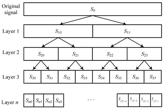
Figure 1.
WPD process.
The WPD of the signal is:
where is the orthogonal scale function; is the orthogonal wavelet function; and and represent the filter coefficients in the multiscale function.
The recursive formula of the wavelet packet coefficient is:
The wavelet packet reconstruction formula is:
where is the n coefficient corresponding to node (i,k) after WPD and node (i,k) represents the k band of layer i.
The WPES improves the stability of the WPD coefficient by extracting the energy of the sub-band to generate the feature vector. According to Parseval’s identity, there is an equal relationship between the wavelet packet energy and the initial energy:
The collected signals are decomposed using the wavelet packet, and the corresponding energy of the j frequency band at layer i is:
where m is the length of the j frequency band and is the n wavelet packet coefficient corresponding to node (i,j) after WPD. The energy spectrum of all nodes was normalized to obtain the feature vectors:
where represents the total energy of each frequency band at layer I after decomposition.
2.2. Deep Belief Networks
A DBN is a deep learning neural network model that is unsupervised and has a multi-layer learning network based on probability statistics. The basic framework of a DBN network comprises restricted Boltzmann machines (RBMs) and works mainly through the training of a hidden layer and a visible layer in the RBM structure, layer-by-layer, constantly updating and optimizing the weight and transfer parameters between layers. While updating and optimizing the parameters layer-by-layer, the tasks of fault feature identification and extraction can be realized, and finally, a fault diagnosis model with a high fault identification accuracy can be established.
As a symmetric network, the RBM is an undirected graph with a bipartite graph structure. The RBM’s fundamental structure is shown in Figure 2. The visible layer v represents the observation data and the hidden layer h can be approximated as the feature extraction layer, with no interlayer connections and complete interlayer connections. W is the weight between layers, is the bias of the visible layer neuron, and is the bias of the hidden layer neuron. In a basic RBM, both the visible layer and hidden layer units are binary variables with and , where 0 represents inactivity and 1 represents activity. All units constitute a state of the RBM, and these states obey a certain distribution.
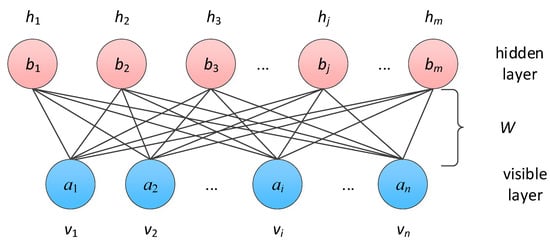
Figure 2.
Structure of RBM.
We assumed that the RBM had n and m neurons located in the visible and hidden layers, respectively. For a given set of (v, h), its energy expression is:
where is an RBM model parameter; is the i neuron’s bias in the visible layer; is the j neuron’s bias in the hidden layer; and is the neuron connection weight.
Equation (10) may be represented by a joint probability distribution for each state (v, h), as illustrated in Equation (11):
where is the dimensional factor. According to the structural characteristics of the RBM, the activation state conditions of each neuron in the hidden layer are independent of each other at a given v.
According to Equation (12), the probability when is activated can be obtained. Because the RBM has symmetric characteristics, the neuron activation probability in the visible layer is given by Equation (13), just as it is for the hidden layer state.
The purpose of RBM training is to find a suitable parameter that fits the given visible layer state. By using a contrastive divergence algorithm, a sufficient approximate can be obtained only by k step Gibbs sampling, and the simple and fast training of the RBM can lay a foundation for the formation of a deep confidence network by stacking the RBM later. The update method of each parameter is as follows:
where is the state distribution of the visible layer reconstruction and is the learning rate.
A DBN is a probabilistic generation model. Figure 3 shows the basic framework structure of the DBN, which is nested with m RBMS and finally nested with a classification layer on the stacked RBMs. DBN training is carried out by training the RBM layer-by-layer. A greedy algorithm is used to conduct fully unsupervised training on the RBM one-by-one, and the back propagation algorithm is used to perform supervised fine-tuned training.
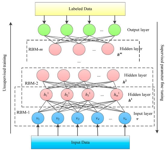
Figure 3.
Structure of DBN.
2.3. Sparrow Search Algorithm
The SSA establishes mathematical models based on the behavior and actions of organisms in the ecological environment. This method solves the global optimum issue by simulating the foraging and anti-hunting behavior of sparrows. Its advantages are that it has fewer control parameters and that the principle is simple and easy to understand. After experimental verification, the sparrow search algorithm is stable and efficient, and can effectively solve global optimization problems. It also provides a new approach and method for most local optimization problems. In order to make the implementation of the algorithm simple, efficient, and easy to explain, researchers formulated the following rules and idealized sparrow behavior when constructing the mathematical model of SSA:
- Explorers in sparrows generally have better fitness, are responsible for searching for food during the foraging process, and transmit the information of foraging direction and location to the followers.
- In the process of foraging, when individual sparrows encounter danger, they will sound an early warning signal. If it exceeds the pre-set safety threshold, explorers will take followers out of the area and find another safe area to continue foraging.
- The identity of explorers and followers in the sparrow population is not fixed. When a follower finds a better foraging place and food source, the individual will shift from follower to explorer, and will also have an equal amount of explorer-into-follower identity, because the calculation presupposes that the proportion of explorers and followers in the whole sparrow population is fixed.
- Since the explorer would arrive at the foraging site first to replenish his energy, the later followers would receive relatively little food. Therefore, the last follower has the worst fitness value, which prompts them to forage elsewhere, optimize their fitness, and increase the exploration of other unsearched areas.
- Followers, after receiving the information from the explorers, will choose to find the explorer with the most food and follow in their footsteps to forage or search around, because they believe that being beside the best explorer is more likely to result in them finding food. Some sparrows will monitor these explorers, and when the explorers find an area with food, they will participate in the competition for food resources.
- When attacked by outsiders, individuals on the edge of the foraging will constantly reposition themselves to the internal safety area. Individual sparrows in the internal safety zones will attempt to approach their peers in order to enhance their safety.
The exact implementation procedure of the SSA is as follows. The randomly generated location matrix X of n sparrows in a d dimensional space is presented below:
where n is the number of sparrows, d represents the dimension of the variable of the problem to be optimized, and represents the position of the j-th sparrow in the i dimensional space.
The current positions of the sparrows and the optimal fitness value were obtained by sorting the population through Formula (16). For the first-generation sparrows, the result obtained was the initial optimal individual. The optimal individual can prioritize access to food:
where f is the fitness value of an individual sparrow.
During the foraging process, the explorer’s position is iteratively updated according to Formula (17):
where Q indicates a random number with a normal distribution; L is the unit row vector; and is a random number in the range of [0, 1].
The update method for the followers’ is as follows:
where indicates the t-th iteration’s global worst position; is the t + 1 generation explorer’s best position; and is a dimensional matrix with dimensional values ranging from 1 to −1 generated at random.
During the iterative optimization process, if 10% to 20% of the total number of sparrows are aware of danger, the impact on the position of all sparrows is as follows:
where is the optimal position in generation t; is the normal distribution step size control parameter, with a mean value of 0 and a variation of 1; is a random number with the value range of [1, 1]; is the fitness value of the current position of the sparrow; and are the global optimal and worst fitness, respectively; and is the minimum value that is not zero.
In order to describe the SSA more succinctly, the flow chart in Figure 4 is used to represent the basic steps of the algorithm.
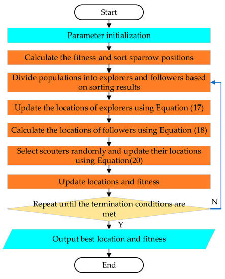
Figure 4.
SSA flow chart.
3. Proposed Methodologies
The relevant weight parameters generated by the DBN network model during the training process were greatly influenced by random factors, and the weight parameters obtained during each training were different. Although the weight parameters will gradually approach the optimal structural parameters during the iterative process, it is also feasible to enter a local optimum state. To alleviate this problem and increase the accuracy of bearing failure diagnostics, the bearing vibration data were processed using a wavelet packet energy spectrum to enhance the characteristic signal. Then, an optimized DBN model was designed. The SSA was utilized to globally optimize the hidden layer nodes and the connection weights between neurons in the DBN using the least error rate of the DBN model as a fitness function, causing the network structure model parameters to swiftly approach the ideal solution. The optimization result was then used as the initial value of the DBN network parameters, which minimized the impact of random factors on the DBN model and enabled the DBN to conduct parameter-iterative training around the optimal solution, making the mapping of neurons more accurate in obtaining feature information and improving the feature extraction performance. We named this method WPES-SSA-DBN, and the algorithm has 6 steps.
Step 1: Create feature vectors. Use a WPES to transform the original vibration signal and extract the sub-band energy. Then, divide the vectors into training and test data.
Step 2: Initialize the SSA population, encode the number of hidden layers and the connection weight between the neurons of the DBN, and set the proportion of explorers and followers in the population.
Step 3: Convert the positional parameter values of sparrow individuals in the SSA into a parameter matrix, replace the relevant parameters of the DBN, and then train and test the DBN. Use the minimum error rate of the DBN, shown in Equation (21), as the fitness function value to return to the SSA:
where represents the prediction label, represents the true label, is the same number as both, and represents the sample number.
Step 4: Update the location of the explorers, followers, and scouters in the SSA values according to Equations (17)–(20). Then, assign the updated sparrow individuals to the DBN and iteratively update to obtain the fitness value.
Step 5: Compare and sort the fitness values to obtain a minimum set of sparrow individual location parameters, which are the corresponding optimal sparrows and also the optimal parameters of the DBN model.
Step 6: Allow the optimized DBN parameters to be self-adjusted according to the original network structure, and then fine-tuned to construct a new improved DBN model for fault diagnoses of the test dataset.
The WPES-SSA-DBN flow chart is given in Figure 5.
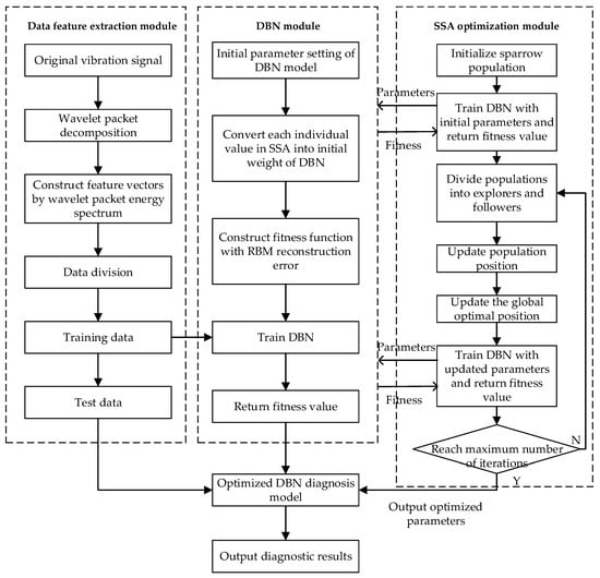
Figure 5.
WPES-SSA-DBN flow chart.
4. Experimentation
4.1. Experimental Environment
Table 1 is the experimental environment for the fault diagnosis experiment using the WPES-SSA-DBN model.

Table 1.
Experimental environment.
4.2. Experimental Dataset
The experimental dataset used Case Western Reserve University (CWRU)’s motor rolling bearing failure data [42]. Figure 6 depicts the structure of the simulated testing bench, which comprised a motor, a torque sensor, a power test meter, and an electronic controller. The testing bench used a 2 hp reliance electric motor to drive a loading mechanism with bearings through a coupling. Highly sensitive piezoelectric acceleration sensors were used to capture small vibration signals of the bearings at a frequency of 12,000 Hz. The bearing to be examined supported the motor’s rotational shaft. Bearings with a single point of damage using electro-discharge machining were separated into four stages of failure damage: 0.1778 mm, 0.3556 mm, and 0.5334 mm, were located in the inner ring, outer ring, and rolling body of the bearing, respectively. In this paper, the input data consisted of 10 categories in the 1 hp load state, whose states and label descriptions are shown in Table 2.
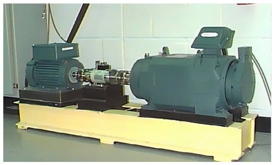
Figure 6.
CWRU bearing experimental bench.
Table 2.
Explanation of experimental data in 10 categories.
4.3. Results and Discussion
To verify the effectiveness of the proposed model in bearing defect diagnoses, four states of signal data, NOR, IR007, OR007, and BA007, with label values of 1,2,5, and 8 were chosen from Table 2. Figure 7 displays the vibration signals for the four states. The vibration signal dataset was composed of 100 data points for each signal, with 70% in the training set and 30% in the test set.
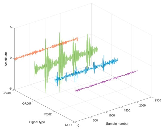
Figure 7.
Time-domain waveforms of rolling bearings for 4 states.
The signals for the four states of rolling bearings were divided into eight layers using the wavelet basis function of db3 to obtain the decomposition coefficients and reconstruction coefficients, which were then used to reconstruct the fault signal feature vectors. Finally, the energy of the 256 sub-bands was obtained, and the energy ratio of each band was analyzed. Figure 8 shows the first eight wavelet packet components of NOR. The horizontal coordinate was the sampling number of the vibration signal and the vertical coordinate was the amplitude after WPD. The energy proportions of the 256 sub-bands are shown in Figure 9. The test dataset was finally converted into 400 × 256 feature vectors by a WPES conversion.
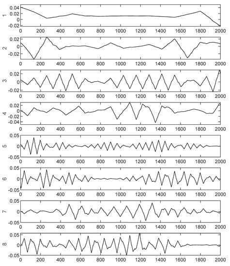
Figure 8.
The first 8 wavelet packet components of NOR.
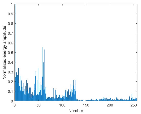
Figure 9.
WPES of NOR.
The t-distribution stochastic neighbor embedding (t-SNE) feature visualization technique was used to downscale and map the input, intermediate, and output layers of the DBN in the WPES-SSA-DBN to a two-dimensional space. With the input and output feature vectors of each DBN layer as the source domain and the expected result of the test set fault diagnosis as the target domain, the diagnosis effect is shown in Figure 10. The four colors represent samples of the different states. From the visualized scatter plot of the WPES features in Figure 10a, the features of the states started to cluster after WPES decomposition, but there was still overlap, and the classification effect was more accurate when extracted layer-by-layer by the optimized DBN module, as shown in Figure 10b,c. Figure 10d shows that the output layer of the WPES-SSA-DBN model can effectively distinguish the signals in the four states.
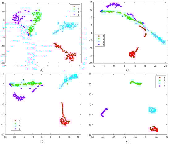
Figure 10.
The t-SNE characteristic downscaling comparison chart of 4 states of the bearing failure training set. (a) Input data: 280 × 256 feature vectors. (b) First layer of DBN output data: 280 × 100 feature vectors. (c) Second layer of DBN output data: 280 × 50 feature vectors. (d) Output data: 280 × 10 feature vectors.
Figure 11 is the test set validation results, where the horizontal coordinate represents a sample and the vertical coordinate represents the label category; the real state of the sample is represented by ‘o’ and the model diagnostic identification result is represented by *. If the real state label agreed with the model diagnostic identification result, the two identifications overlapped and the WPES-SSA-DBN model achieved 100% accuracy in identifying the four types of vibration states of bearings. During the experiments, four typical fault diagnosis methods were used for comparison, namely an SVM, an ELM, a GA-BP, and a DBN. In addition, all test models were tested 10 times independently to reduce the effect of random errors. Table 3 shows the diagnostic statistics of the test sets for the four states, including the maximum accuracy, minimum accuracy, mean, and standard deviation. From the comparison results, it can be seen that, with a small sample type, the average fault diagnosis rate of all five methods exceeded 93%, while the accuracy of the WPES-SSA-DBN reached 100%. Compared with the other methods, the standard deviation of the WPES-SSA-DBN was 0, indicating that the model achieved a 100% correct diagnostic rate in all 10 experiments.
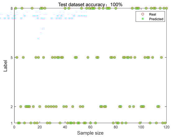
Figure 11.
Graph of the test set identification results for the 4 states.
Table 3.
Recognition effect of the verification set for the 4 states under different methods.
To continue to validate the classification capability of the WPES-SSA-DBN, the diagnostic labels were increased from four to ten states, as shown in Table 2. A total of 100 data points were taken from each state of labels to form a total of 1000 datasets, of which 70% were allocated to the training set and 30% to the test set.
In Figure 12, after increasing the data volume and data type, the overlap of the feature data gradually decreased after the layer-by-layer extraction by the DBN module. After being processed by the WPES-SSA-DBN model, these features were effectively distinguished and clustered in the corresponding regions, which indicated that the proposed model can mine representative high-order features from the signal.
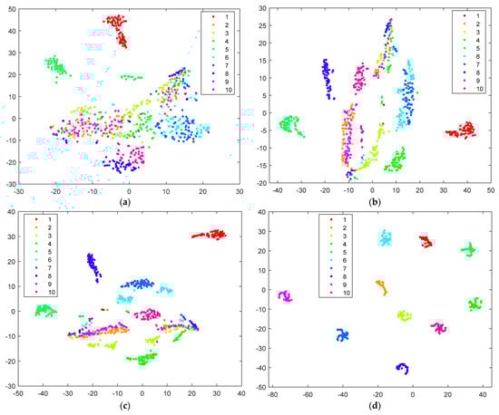
Figure 12.
The t-SNE characteristic downscaling comparison chart of 10 types of bearing failure training sets. (a) Input data: 700 × 256 feature vectors. (b) First layer of DBN output data: 700 × 100 feature vectors. (c) Second layer of DBN output data: 700 × 50 feature vectors. (d) Output data: 700 × 10 feature vectors.
The diagnostic results of the WPES-SSA-DBN for the 10 states of the test set are shown in Figure 13. Out of 300 data, 298 were diagnosed correctly, with an accuracy rate of 99.33%. Table 4 lists the diagnostic statistics of the test set for the 10 states, and the WPES-SSA-DBN had the highest average accuracy and the smallest standard deviation, indicating that the model had a better recognition accuracy and stability. In addition, combined with the results shown in Table 4, the average correct rate of the SVM was the lowest, which also indicates that the deep-learning-based fault diagnosis algorithm was more advantageous for the same fault types.
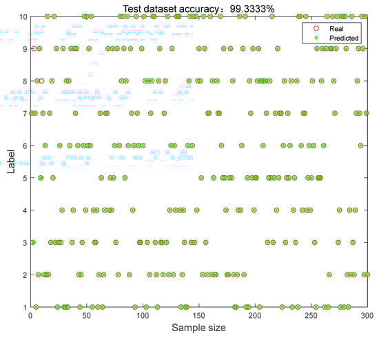
Figure 13.
Graph of the test set identification results for the 10 states.
Table 4.
Recognition effect of the test set for the 10 states under different methods.
5. Conclusions, Limitations, and Future Research
Rolling bearings are one of the most vulnerable sections of rotating machinery. Accurate fault identification can provide equipment with accurate maintenance and effectively reduce the negative impact of bearings on mechanical equipment. In this paper, the WPES-SSA-DBN was proposed to diagnose bearing fault types. The model decomposed the original vibration signal into distinct frequency bands using a wavelet packet transform, retained the original signal frequency information completely, and constructed feature vectors by extracting the energy of sub-bands through the WPES. Then, the SSA was used to perform a global search for the connection weights between neurons and the number of nodes in the hidden layer of the DBN using the minimization error rate as the fitness function, so that the DBN was trained around the optimal solution with iterative parameters to improve the feature extraction performance. Finally, rolling bearing data from CWRU were selected for validation, and two sets of experiments were conducted to carry out diagnoses for four and ten types of fault data. The t-SNE technique was used in the experiments to visualize the feature extraction of the proposed model in two dimensions, and the results showed that the proposed model can effectively distinguish different features. An SVM, ELM, GA-BP, and DBN were selected as the comparison methods, and the diagnostic results showed that the diagnostic accuracy of the WPES-SSA-DBN reached 100% and 99.34% for the two experiments, with the smallest standard deviation. The experimental results show that the WPES-SSA-DBN can choose better training parameters and has obvious advantages in classification performance recognition accuracy compared with the comparison model, which can accurately achieve the fault classification identification of rolling bearings.
The research of data-driven intelligent fault diagnosis technology has been given much attention in the industry and fruitful research results have been achieved. This paper aimed to investigate the vibration signal from a single-fault rolling bearing. However, in many cases, collected vibration signals are often multi-fault, and even multi-fault coupling phenomena of different types in different parts occur. Therefore, more detailed intelligent diagnostic methods for compound faults will be studied in the future to achieve the accurate identification of multiple fault types in bearings and further enrich and develop rolling bearing compound fault diagnostic techniques and methods.
Author Contributions
Methodology, J.Q. and X.C.; formal analysis, P.L.; writing—original draft preparation, J.Q.; writing—review and editing, L.Z. and X.M. All authors have read and agreed to the published version of the manuscript.
Funding
This research was funded by the Key Scientific and Technological Project of Henan Province (232102241027, 232102220092), the Industry–University Cooperative Education Program of the Ministry of Education, (202002029035), the Key Scientific Research Projects of the Higher Education Institutions of Henan Province (23B460008), and the Doctoral Fund of Henan Institute of Technology (KY1750).
Data Availability Statement
The data presented in the experiments may be available from the first author upon request.
Conflicts of Interest
The authors declare no conflict of interest.
References
- Chen, H.; Jiang, B. A review of fault detection and diagnosis for the traction system in high-speed trains. IEEE Trans. Intell. Transp. Syst. 2019, 21, 450–465. [Google Scholar] [CrossRef]
- Sun, Q.; Xiong, J.; Zhang, Q. Research methods of the rotating machinery fault diagnosis. Mach. Tool Hydraul. 2018, 46, 133–139. [Google Scholar] [CrossRef]
- Rehman, N.; Afta, H. Multivariate variational mode decomposition. IEEE Trans. Signal Process. 2019, 67, 6039–6052. [Google Scholar] [CrossRef]
- Khalid, S.; Song, J.; Raouf, I.; Kim, H. Advances in Fault Detection and Diagnosis for Thermal Power Plants: A Review of Intelligent Techniques. Mathematics 2023, 11, 1767. [Google Scholar] [CrossRef]
- Han, T.; Liu, R.; Zhao, Z.; Kundu, P. Fault Diagnosis and Health Management of Power Machinery. Machines 2023, 11, 424. [Google Scholar] [CrossRef]
- Ding, X.; He, Q.; Luo, N. A fusion feature and its improvement based on locality preserving projections for rolling element bearing fault classification. J. Sound Vib. 2015, 335, 367–383. [Google Scholar] [CrossRef]
- Rostaghi, M.; Azami, H. Dispersion Entropy: A Measure for Time-Series Analysis. IEEE Signal Process. Lett. 2016, 23, 610–614. [Google Scholar] [CrossRef]
- Lei, Y.; Lin, J.; Zuo, M. Condition monitoring and fault diagnosis of planetary gearboxes: A review. Measurement 2014, 48, 292–305. [Google Scholar] [CrossRef]
- Lee, C.; Le, T.; Chang, C. Application of Hybrid Model between the Technique for Order of Preference by Similarity to Ideal Solution and Feature Extractions for Bearing Defect Classification. Mathematics 2023, 11, 1442. [Google Scholar] [CrossRef]
- Hoang, D.; Kang, H.; Kang, J. A motor current signal-based bearing fault diagnosis using deep learning and information fusion. IEEE Trans. Instrum. Meas. 2020, 69, 3325–3333. [Google Scholar] [CrossRef]
- Lian, Z.; Zhou, Z.; Zhang, X.; Feng, Z.; Han, X.; Hu, C. Fault Diagnosis for Complex Equipment Based on Belief Rule Base with Adaptive Nonlinear Membership Function. Entropy 2023, 25, 442. [Google Scholar] [CrossRef] [PubMed]
- Evgeny, A.; George, V.; Irina, S.; Alexander, P. An Overview of Vibration Analysis Techniques for the Fault Diagnostics of Rolling Bearings in Machinery. Shock Vib. 2022, 2022, 6136231. [Google Scholar] [CrossRef]
- Antonino, J.; Pons, J.; Lee, S. Advanced rotor fault diagnosis for medium-voltage induction motors via continuous transforms. IEEE Trans. Ind. Appl. 2016, 52, 4503–4509. [Google Scholar] [CrossRef]
- Chuan, L.; Oliveira, J.; Cerrada, M.; Cabrera, D.; Sánchez, R.; Zurita, G. A systematic review of fuzzy formalisms for bearing fault diagnosis. IEEE Trans. Fuzzy Syst. 2019, 27, 1362–1382. [Google Scholar] [CrossRef]
- Feng, Z.; Liang, M.; Chu, F. Recent advances in time-frequency analysis methods for machinery fault diagnosis:a review with application examples. Mech. Syst. Signal Process. 2013, 38, 165–205. [Google Scholar] [CrossRef]
- Attoui, I.; Fergani, N.; Boutasseta, N.; Oudjani, B.; Deliou, A. A new time-frequency method for identification and classification of ball bearing faults. J. Sound Vib. 2017, 397, 241–265. [Google Scholar] [CrossRef]
- Paulis, F.; Boudjefdjouf, H.; Bouchekara, H.; Orlandi, A.; Smail, M. Performance improvements of wire fault diagnosis approach based on time-domain reflectometry. IET Sci. Meas. Technol. 2017, 11, 538–544. [Google Scholar] [CrossRef]
- Han, W.; Wang, Z.; Shen, Y.; Xie, W. Robust fault estimation in the finite-frequency domain for multi-agent systems. Trans. Inst. Meas. Control 2019, 41, 3171–3181. [Google Scholar] [CrossRef]
- Karioja, K.; Lahdelma, S.; Litak, G.; Ambrozkiewicz, B. Extracting periodically repeating shocks in a gearbox from simultaneously occurring random vibration. In Proceedings of the 15th International Conference on Condition Monitoring and Machinery Failure Prevention Technologies, CM/MFPT, Nottingham, UK, 10–12 September 2018; pp. 456–464. [Google Scholar]
- Duan, Y.; Wang, C.; Chen, Y.; Liu, P. Improving the Accuracy of Fault Frequency by Means of Local Mean Decomposition and Ratio Correction Method for Rolling Bearing Failure. Appl. Sci. 2019, 9, 1888. [Google Scholar] [CrossRef]
- Burriel, J.; Puche, R.; Pineda, M. Short-Frequency Fourier Transform for Fault Diagnosis of Induction Machines Working in Transient Regime. IEEE Trans. Instrum. Meas. 2017, 66, 432–440. [Google Scholar] [CrossRef]
- Qin, Y.; Mao, Y.; Chen, H. M-band flexible wavelet transform and its application to the fault diagnosis of planetary gear transmission systems. Mech. Syst. Signal Process. 2019, 134, 106298. [Google Scholar] [CrossRef]
- Yan, B.; Wang, B.; Zhou, F.; Li, W.; Xu, B. Sparse feature extraction for fault diagnosis of rotating machinery based on sparse decomposition combined multiresolution generalized S transform. J. Low Freq. Noise Vib. Act. Control 2019, 38, 441–456. [Google Scholar] [CrossRef]
- Lv, Q.; Yu, X.; Ma, H.; Ye, J.; Wu, W.; Wang, X. Applications of Machine Learning to Reciprocating Compressor Fault Diagnosis: A Review. Processes 2021, 9, 909. [Google Scholar] [CrossRef]
- Fu, S.; Wu, Y.; Wang, R.; Mao, M. A Bearing Fault Diagnosis Method Based on Wavelet Denoising and Machine Learning. Appl. Sci. 2023, 13, 5936. [Google Scholar] [CrossRef]
- Yu, Y.; Gao, H.; Zhou, S.; Pan, Y.; Zhang, K.; Liu, P.; Yang, H.; Zhao, Z.; Madyira, D.M. Rotor Faults Diagnosis in PMSMs Based on Branch Current Analysis and Machine Learning. Actuators 2023, 12, 145. [Google Scholar] [CrossRef]
- Zhang, X.; Jiang, D.; Long, Q.; Han, T. Rotating machinery fault diagnosis for imbalanced data based on decision tree and fast clustering algorithm. J. Vibroeng. 2017, 19, 4247–4259. [Google Scholar] [CrossRef]
- Tang, G.; Pang, B.; Tian, T.; Zhou, C. Fault Diagnosis of Rolling Bearings Based on Improved Fast Spectral Correlation and Optimized Random Forest. Appl. Sci. 2018, 8, 1859. [Google Scholar] [CrossRef]
- Ren, L.; Yong, B. Wind Turbines Fault Classification Treatment Method. Symmetry 2022, 14, 688. [Google Scholar] [CrossRef]
- Qu, J.; Ma, B.; Ma, X.; Wang, M. Hybrid Fault Diagnosis Method based on Wavelet Packet Energy Spectrum and SSA-SVM. Int. J. Adv. Comput. Sci. Appl. (IJACSA) 2022, 13, 52–60. [Google Scholar] [CrossRef]
- Equbal, M.; Khan, S.; Islam, T. Transformer incipient fault diagnosis on the basis of energy-weighted DGA using an artificial neural network. Turk. J. Electr. Eng. Comput. Sci. 2018, 26, 77–88. [Google Scholar] [CrossRef]
- Duan, L.; Xie, M.; Wang, J.; Bai, T. Deep learning enabled intelligent fault diagnosis: Overview and applications. J. Intell. Fuzzy Syst. 2018, 35, 5771–5784. [Google Scholar] [CrossRef]
- Zhu, J.; Jiang, Q.; Shen, Y. Application of recurrent neural network to mechanical fault diagnosis: A review. J. Mech. Sci. Technol. 2022, 36, 527–542. [Google Scholar] [CrossRef]
- Tang, S.; Yuan, S.; Zhu, Y. Deep Learning-Based Intelligent Fault Diagnosis Methods Toward Rotating Machinery. IEEE Access 2020, 8, 9335–9346. [Google Scholar] [CrossRef]
- Jia, P.; Wang, C.; Zhou, F.; Hu, X. Trend Feature Consistency Guided Deep Learning Method for Minor Fault Diagnosis. Entropy 2023, 25, 242. [Google Scholar] [CrossRef] [PubMed]
- Zhang, X.; Li, J.; Wu, W.; Dong, F.; Wan, S. Multi-Fault Classification and Diagnosis of Rolling Bearing Based on Improved Convolution Neural Network. Entropy 2023, 25, 737. [Google Scholar] [CrossRef]
- Zhang, Q.; He, Q.; Qin, J.; Duan, J. Application of Fault Diagnosis Method Combining Finite Element Method and Transfer Learning for Insufficient Turbine Rotor Fault Samples. Entropy 2023, 25, 414. [Google Scholar] [CrossRef]
- Mansouri, M.; Dhibi, K.; Hajji, M.; Bouzara, K.; Nounou, H.; Nounou, M. Interval-Valued Reduced RNN for Fault Detection and Diagnosis for Wind Energy Conversion Systems. IEEE Sens. J. 2022, 22, 13581–13588. [Google Scholar] [CrossRef]
- Jiang, M.; Liang, Y.; Feng, X. Text classification based on deep belief network and softmax regression. Neural Comput. Applic. 2018, 29, 61–70. [Google Scholar] [CrossRef]
- Luo, H.; He, C.; Zhou, J.; Zhang, L. Rolling Bearing Sub-Health Recognition via Extreme Learning Machine Based on Deep Belief Network Optimized by Improved Fireworks. IEEE Access 2021, 9, 42013–42026. [Google Scholar] [CrossRef]
- Yang, E.; Wang, Y.; Wang, P.; Guan, Z.; Deng, W. An Intelligent Identification Approach Using VMD-CMDE and PSO-DBN for Bearing Faults. Electronics 2022, 11, 2582. [Google Scholar] [CrossRef]
- Smith, W.; Randall, R. Rolling element bearing diagnostics using the Case Western Reserve University data: A benchmark study. Mech. Syst. Signal Process 2015, 64–65, 100–113. [Google Scholar] [CrossRef]
Disclaimer/Publisher’s Note: The statements, opinions and data contained in all publications are solely those of the individual author(s) and contributor(s) and not of MDPI and/or the editor(s). MDPI and/or the editor(s) disclaim responsibility for any injury to people or property resulting from any ideas, methods, instructions or products referred to in the content. |
© 2023 by the authors. Licensee MDPI, Basel, Switzerland. This article is an open access article distributed under the terms and conditions of the Creative Commons Attribution (CC BY) license (https://creativecommons.org/licenses/by/4.0/).