Advancing Fault Prediction: A Comparative Study between LSTM and Spiking Neural Networks

Abstract

Predicting system faults is critical to improving productivity, reducing costs, and enforcing safety in industrial processes. Yet, traditional methodologies frequently falter due to the intricate nature of the task. This research presents a novel use of spiking neural networks (SNNs) in anticipating faults in syntactical time series, utilizing the generalized stochastic Petri net (GSPN) model. The inherent ability of SNNs to process both time and space aspects of data positions them as a prime instrument for this endeavor. A comparative evaluation with long short-term memory (LSTM) networks suggests that SNNs offer comparable robustness and performance.

1. Introduction

Failure prediction is a significant research topic in the field of industrial process safety. It serves as a mechanism to enhance system performance and reduce business costs by preventing undesired malfunctions that could potentially cause harm to the local community, employees, and the environment [1]. The literature contains several works proposing various techniques and algorithms to address this task across multiple domains. The literature contains several works proposing various techniques and algorithms to address this task across multiple domains. For example, ref. [2] recommended deploying the machine learning model Catboost for financial distress prediction. Alternatively, ref. [3] exploited the gradient-boosting model XGBoost to anticipate respiratory failures in COVID-19 patients within 48 h. Autonomous driving model failures were forecasted by [4] employing convolutional neural networks (CNNs) and recurrent convolutional neural networks (RCNNs).

While the majority of existing approaches in the literature employ conventional neural networks, including multi-layer perceptrons, CNNs, RNNs, and LSTMs, for the purpose of conducting failure prediction in time series data, a segment of the scientific community is gradually embracing the so-called third generation of neural networks known as spiking neural networks (SNNs). This type of network has demonstrated promising outcomes, mainly when applied to problems involving sparse data, such as system failures, where most of the algorithms have difficulties due to the imbalanced nature of the data.

For software defect prediction, ref. [5] utilized an SNN, leveraging smoothed versions of the input and output spike trains and computing an approximate gradient of the error function. In an innovative approach, ref. [6] developed an end-to-end pipeline for anomaly alerts, including cochlea models to decompose the signals into frequency channels, translating them into spike trains via a delta modulator, and finally applying SNNs for detecting channel-wise deflection rates indicative of a transition from a healthy to an unhealthy state.

An unsupervised approach to anomaly discovery was proposed in [7]; based on the online evolving spiking neural network classifier [8], the authors built a new algorithm, wherein rather than dividing the output neurons into distinct classes, each output neuron is assigned to an output value and posteriorly updated during the network training. For detecting high-frequency oscillations (HFOs) in epilepsy surgeries, ref. [9] used an SNN application based on a hardware implementation algorithm, obtaining promising results, while [10] applied an SNN for diagnosing faults in bearing for rotating machinery.

SNNs have also demonstrated their prowess in the realm of image recognition. For instance, ref. [11] integrated SNNs with convolutional neural networks and autoencoders for skin cancer detection through image classification. An algorithm for accelerating the training of deep SNNs was proposed in [12]. The authors used the network for handling dynamic vision sensors. Taking advantage of the natural ability of the SNNs to handle sparse events, researchers in [13] proposed the use of this kind of network for radar gesture recognition. They were able to achieve a 93% accuracy rate using only one convolutional layer and two fully connected hidden layers.

SNNs has also been used for performing classical tasks of machine learning such as classification and regression, having comparable performance to the traditional artificial neural networks (ANNs) and, in some cases, higher performance. For instance, ref. [14] applied a deep SNN for large vocabulary automatic recognition using speech audios. Researchers utilized electroencephalograph (EEG) signals in conjunction with SNNs for emotion classification [15], and motor task classification in EEG signals [16]. Furthermore, a self-normalized SNN was employed for pan-cancer classification [17], and an SNN solution was incorporated into neuromorphic hardware for real-time classification in rank-order spiking patterns, providing a time-efficient solution for data pattern drift detection [18].

The utility of spiking neural networks (SNNs) spans a wide range of applications. For example, ref. [19] proposed an event-based regression model using a convolutional SNN trained via the spike layer error reassignment in time (SLAYER) for estimating the angular velocity of a rotating event camera. Similarly, ref. [20] employed a multilayer SNN in conjunction with event-based cameras for predicting ball trajectories, training the network using the spike-timing-dependent plasticity (STDP) learning rule. SNNs also find valuable applications in unsupervised tasks as demonstrated by [21], who proposed a clustering-based ensemble model for air pollution prediction using evolving SNNs. This process involves segmenting the time series samples into K distinct groups and subsequently creating and training an SNN for each cluster to predict values.

Motivated by the promising potential observed in the research context, the authors of this work decided to apply SNNs for fault prediction. In particular, in this work, a network architecture consisting of leaky integrate-and-fire (LIF) neurons was chosen. The selection of LIF neurons was driven by their advantageous characteristics, which include low complexity and high computational efficiency. To implement the proposed model, the authors used a Python simulator NengoDL, a tool for simulating training Nengo models. This simulator was originally introduced by [22], and it is based on the neural engineering framework (NEF) [23].

In order to leverage the intrinsic temporal–spatial characteristics of spiking neural networks (SNNs), the authors of this work used synthetic sparse binary and ternary times series data. These data were generated by simulating a generalized stochastic Petri net (GSPN) and used as input for the network. The results obtained from this study demonstrate that the SNNs can emerge as a robust contender against regular ANNs in fault detection tasks, having high accuracy and recall, even when there is drift in the test data.

The remainder of this work is structured as follows: Section 2 provides an overview of the fundamental concepts necessary to comprehend spiking neural networks (SNNs). Section 3 outlines the methodology employed in this study, including a detailed explanation of the proposed approach and the data generation process. Section 4 presents the obtained results and compares them to the long short-term memory (LSTM) approach. The concluding remarks and insights derived from this study are presented in the final section, which summarizes the key findings, highlights the conclusions drawn from the research, and outlines potential future research directions to further advance the current work.

2. Spiking Neural Networks

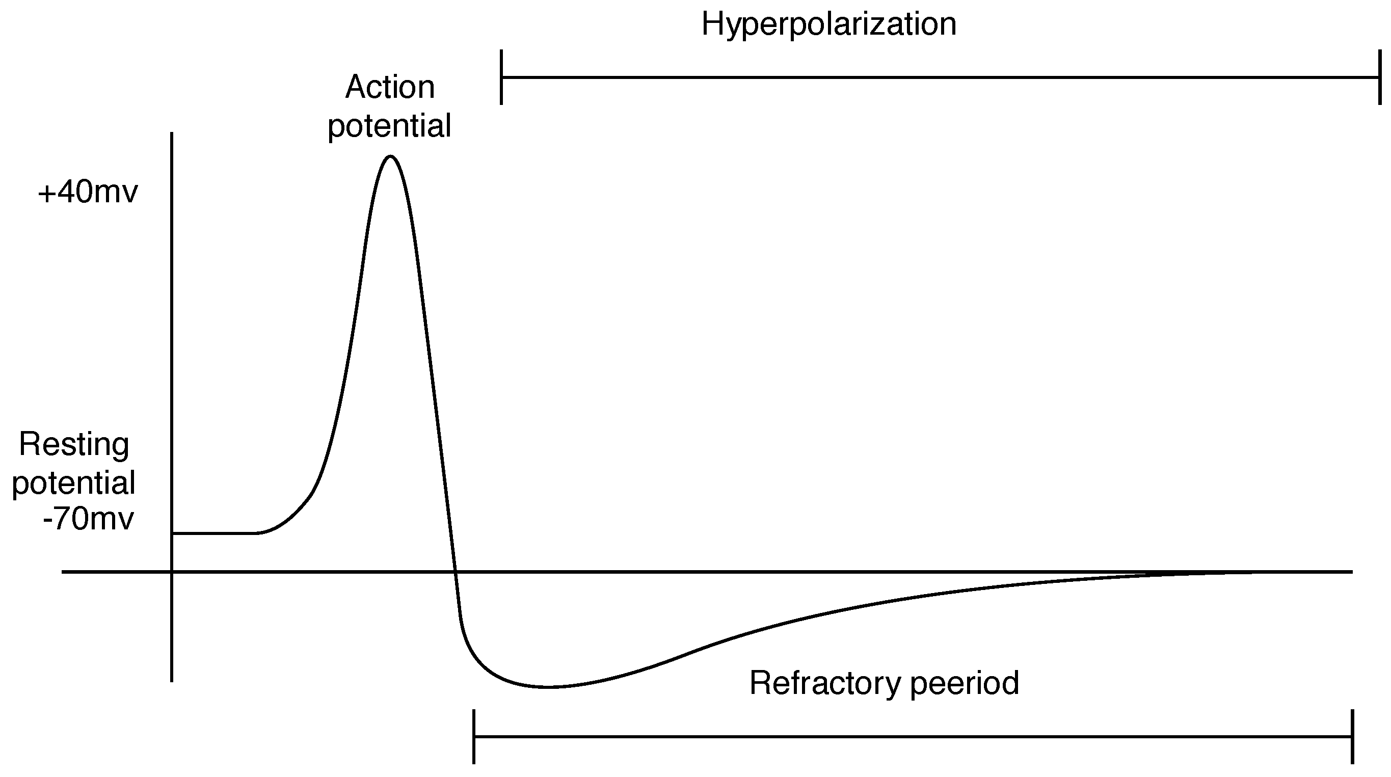
Considered to be the third generation of artificial neural networks, spiking neural networks were inspired by the neurobiological characteristics of the human brain [24]. Unlike conventional ANNs, neurons in SNNs do not activate in every learning cycle. Instead, only those that reach a certain membrane voltage threshold are activated, a process known as neuron firing or spiking.

This spike can be conceptualized as an electrical impulse akin to the behavior of the Dirac delta function. It is an event that occurs when the membrane potential of a neuron surpasses a specific level of charge (voltage), also called the threshold. In biological terms, it is possible to say that the membrane potential is the difference between the electrical potential on the interior of the cell and its exterior [25]. A mathematical representation of a spike is provided in Equation (1):

$$\begin{array}{c}\delta \left(t\right)=1, fort=0\hfill \\ \delta \left(t\right)=0, otherwise\hfill \end{array}$$

(1)

From a biological context, it is said that the learning process occurs from an exchange of electrical and chemical signals from one or more neurons to other neurons. This occurs through a structure called synapse. The neuron that sends the signal is called a presynaptic neuron, whereas the neuron that receives the spike is called a postsynaptic neuron [26]. Each signal sent is then processed and contributes to the membrane potential of the neuron. Consequently, the neuron accumulates potential until it surpasses its intrinsic threshold. At this point, the neuron generates and emits an action potential, commonly referred to as a spike. This spike serves as a fundamental unit of information processing within the spiking neural network.

What the SNNs intend to do is to mimic this biological behavior. In these networks, the weights represent the synapses. The neuron definition is also inspired by the biological neuron characteristics, having the attributes such as potential, threshold, and refractory time, among others.The main idea of SNNs is to replicate the dynamics of the learning process. The most known example of this approximation is the strengthening or weakening of the synapses, which are replicated by adjusting the network weights [27].

In the dynamics of neural functioning, after a neuron fires, it enters a refraction period. While in refraction, the neuron cannot fire any other spike. This phase is known as hyperpolarization, and at the end of it, the neuron potential holds a voltage of approximately −70 mV. This voltage is called the resting potential. Figure 1 shows a graphic of the membrane potential over time.

Among the most recognized models that attempt to mimic the behavior of spiking neurons are the leaky integrate-and-fire (LIF), Izhikevich, and Hodgkin–Huxley models. All these models mimic the membrane potential dynamics of individual and networks of neurons, at different levels of abstraction, including the formation of the action potential. In each of these models, both the input and output are action potentials. The next subsection of this paper explains some of the main concepts of the LIF neuron model.

Leaky Integrate and Fire

The LIF model describes the dynamics of the accumulation of the membrane potential of a neuron, denoted as $u_i\left(t\right)$, through the integration (or summation) of its inputs over time. The threshold of the neuron is set as a fixed value, $\vartheta$. When the membrane potential reaches this level of charge, a spike is fired. It is worth noting that in this type of model, the shape of the spike is not important to describe the information of it but the specific time $t_i$ that the neuron fired.

The model can be mathematically characterized by two components: a linear differential equation for the neuron’s membrane potential and a firing mechanism. Depicting the neuron as an electrical circuit allows us to represent it as a resistor capacitor (RC) circuit, with the current serving as the network input. The fundamental premise is that the capacitor is charged through the input current in this circuit, and its potential is the membrane potential. When the current disappears, the capacitor’s voltage reverts to the resting potential.

In this study, the authors employ an SNN consisting of leaky integrate-and-fire (LIF) neurons to tackle the task of failure prediction in a synthetic dataset. The obtained results are compared with those of a traditional approach, serving as a benchmark for performance evaluation. The comparison encompasses both the predictive accuracy of the models.

3. Proposed Methodology

This study’s primary aim is to introduce the use of spiking neural networks (SNNs) for fault detection in industrial systems. To emulate the system behavior, the authors utilized the mathematical modeling language provided by the Petri network graph model, incorporating generalized stochastic networks (GSPNs). This approach facilitated the creation of a network that replicates the dynamic behavior of the industrial systems. Both systems reproduce established models within the field of dependability, encompassing reliability and availability models [28,29]. In these kinds of models, the system states are controlled by probabilities of failure and repair. By utilizing exponentially timed transitions, the authors were able to model system events such as failure and recovery. Subsequently, the network was simulated to generate the training dataset for the SNN model.

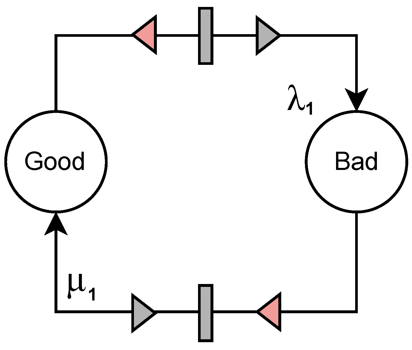
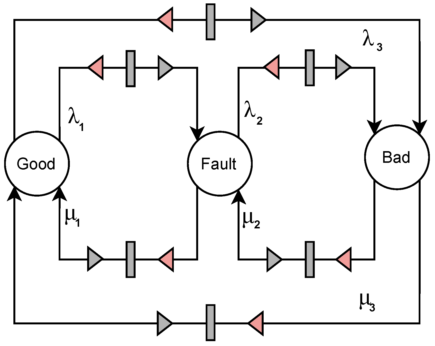
Our approach intends to investigate systems of varying complexity levels, employing two distinct system representations. The first representation comprises a binary classification problem with two states, Good (operational) and Bad (non-operational), reflecting a simpler system with the goal of differentiating between functional and non-functional states. The second representation is a ternary classification problem involving three states, Good (operational), Fault (damaged but still operational), and Bad (nonoperational), depicting a more complex system with the objective to differentiate among various operational states, including faulty ones.

The SNN implementation in this study relied on the NengoDL framework and Nengo implementations of neurons. This framework facilitates the modeling of SNNs and has been used in some applications in the scientific community, such as in [30,31], for modeling SNNs. One of the notable advantages of this framework is its ability to construct architectures similar to those offered by TensorFlow. Consequently, developers can define layers and their interconnections, as well as specifying neuron types and associated parameters, including the refractory time constant, amplitude, and circuit RC time constant, among others. Additionally, models constructed with this framework can be effortlessly deployed on neuromorphic hardware [32].

In this experimental study, the performance evaluation of both networks was conducted using statistical metrics, such as accuracy, F1-score, and recall scores. The parameter settings for generating system simulations for GSPN Network 1 (mimicking the simpler system) and GSPN Network 2 (mimicking the more complex Systes) are presented in

Table 1. Petri Network 1 (two-state system)—simulation parameters.

	Frequency
Failure transition—$\lambda$	3 months (2160 h)
Recovery transition—$\mu$	3 days (72 h)
simulation time	5 years (42,300 h)

and

Table 2. Petri Network 2 (three-state system)—simulation parameters.

	Frequency
Failure transition—${\lambda }_1$	720 h (Monthly)
Failure transition—${\lambda }_2$	15 days (360 h)
Failure transition—${\lambda }_3$	3 months (2160 h)
Recovery transition—${\mu }_1$	3 days (72 h)
Recovery transition—${\mu }_2$	3 days (72 h)
Recovery transition—${\mu }_3$	5 days (120 h)
Simulation time	5 years (42,300 h)

, respectively. Additionally, to investigate the behavior of the SNN model in the presence of outlier events, an additional experiment was incorporated into the evaluation of the trained model for the second system. The primary objective was to analyze the distinct operating profiles of the proposed SNN model. Therefore, Model 2 was also tested under three different data scenarios:

• Using data from a system where a fatal crash can occur every six months.
• Using data from a system where a fatal crash can occur annually.
• Using data from a system where a fatal crash can occur every two years.

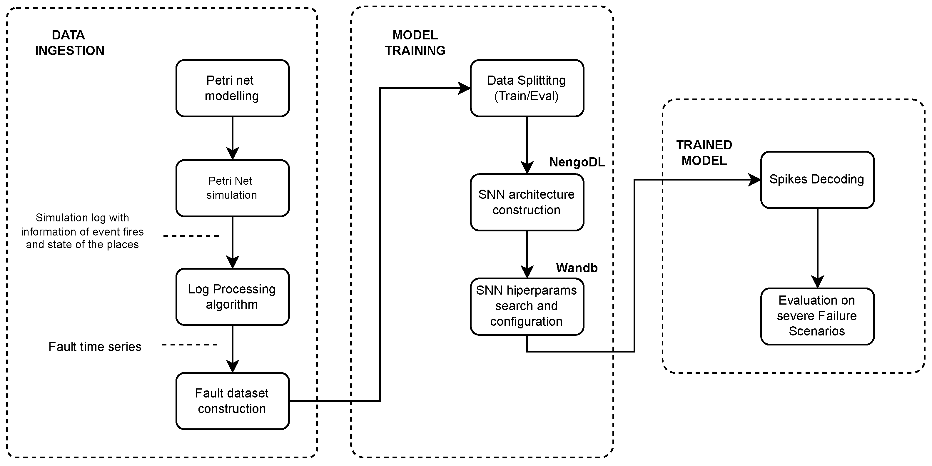
Concluding the experiment, this paper also performed a comparison between the SNN results and the long-short-term memory (LSTM) results in the same analyzed scenarios. For a better understanding, Figure 2 shows a complete flow chart of the methodology applied in this work, and the following subsections describe the data ingestion and model training processes.

3.1. Data Ingestion

This section provides a detailed description of the processes used to generate the dataset utilized for training both SNN and LSTM models. It explores the fundamentals of Petri nets and elaborates on the characteristics of each network, including input and output gateways, as well as transition probabilities. Additionally, it delves into the log-processing task developed to transform the network’s output into a time series format.

3.1.1. Petri Nets Modeling and Simulation

Petri networks, originally proposed by Petri in his work [33], serve as a modeling approach for capturing the dynamics of information within distributed systems. These networks are visually represented as directed graphs, wherein the nodes are referred to as places, and the edges represent the information pathways governed by transitions. Notably, Petri networks are bipartite graphs, which implies that places are exclusively connected to transitions, and transitions are exclusively connected to places.

Each place has the capacity to store one or more tokens, represented by black dots [34]. For a transition to occur, it requires at least one token to be present in the input place. Upon the execution of the transition, the token is removed from the source place and placed into the designated destination place. In order to incorporate temporal considerations into Petri nets, probabilistic characteristics were introduced, resulting in a modified version known as generalized stochastic Petri nets (GSPNs) [35,36].

In this kind of network, it is possible to assign probabilities to transitions, determining the likelihood of their occurrence. This probability is computed using an exponential distribution, which is associated with a specific firing rate. Thus, if a transition $T_1$ has a firing rate ${\lambda }_1$, it will fire at time $t_i$ with an exponential distribution with a mean $\frac{1}{{\lambda }_1}$.

In this work, the formalism of the stochastic activity networks (SANs) was used to model the system behavior. In this formalism, in addition to the traditional structures of Petri nets, SANs introduce input and output gateways that facilitate the modeling of transitions between places. The input gateways define the marking changes that will occur when a transition is fired. To do so, they use an input predicate, which is a Boolean function that defines its behavior. The output gateways specify the marked changes on the Petri network after a transition has occurred.

In the context of failure analysis, the duration for which a system remains operational before experiencing a failure is commonly known as the mean time to failure (MTTF). Conversely, the duration required to restore a failed system to its operational state is referred to as the mean time to repair (MTTR). Thus, in the systems modeled in this experiment, the failure and recovery events were set using the parameters $\lambda$ (time to failure), and $\mu$ (time to recover).

As previously stated, this work used stochastic Petri network simulations to produce the training datasets. To produce each dataset, the authors processed the log file outputted by the Petri net simulator, using a custom-developed algorithm using natural language processing concepts. This algorithm transformed the log file into a continuous time series reflecting the system behavior during the simulation.

Figure 3 and Figure 4 show the net structure designed for systems 1 and 2, respectively. Table 1 and Table 2 show the settings for $\lambda$ and $\mu$ for each system simulation. It is worth noticing that in System 2, there are three failure rates, ${\lambda }_1$, ${\lambda }_2$, and ${\lambda }_3$, which are associated with the transitions from the states Good to Fault, Fault to Bad, and Good to Bad, respectively. Similarly, there are also three recovery rates, ${\mu }_1$, ${\mu }_2$, and ${\mu }_3$, associated with the transitions Fault to Bad, Bad to Fault, and Bad to Good, respectively. In the context of this experiment, the authors used a single token for both Petri networks; the initial state was set as Good (operational), meaning that the systems always start operations from a state of proficient functionality. Furthermore, all transitions were configured following an exponential distribution, which is defined by the rate parameter. The specific values utilized for setting all the transition rate parameters for both Systems 1 and 2 are shown in Table 1 and Table 2, respectively, in the results section.

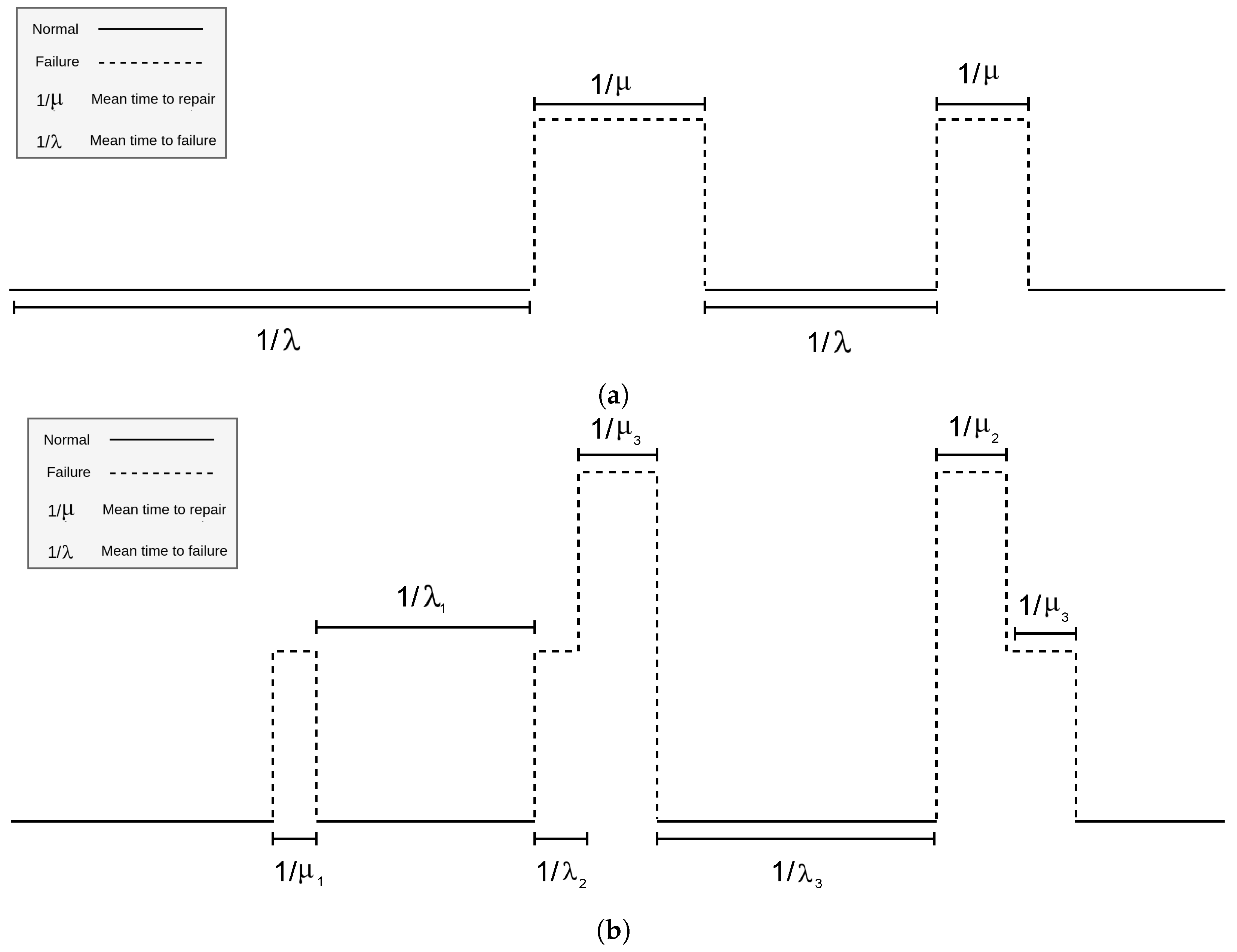
For a better understanding of the signal that can be extracted from the simulations of GSPNs, the behavioral depiction of both systems is illustrated in Figure 5. In Figure 5a, the behavior of System 1 is shown, whereas the behavior of System 2 is delineated in Figure 5b. For both systems, the duration of the failure and recovery states is probabilistically defined by the set rates $\lambda$ and $\mu$, respectively. It is worth noting that in the case of System 2, given its two tiers of failure, the authors chose to visually represent the failure levels with different heights, facilitating a straightforward comprehension of the transitions from one failure level to another.

3.1.2. Log Processing Construction

The software Möbius [37] was utilized for modeling and simulating the GSPNs. Möbius offers a platform for GSPN analysis and presents the ability to integrate C++ code to outline the behavior of the input and output gates, which are essential for dynamically managing network transitions. It further allows the definition of the simulation time and the desired confidence interval in the results. For this study, the authors established a simulation period of five years, with ten repetition batches and a confidence level of 0.95. Each simulation for both systems is parameterized according to the specifications exhibited in Table 1 for System 1 with two states, and Table 2 for System 2 with three states.

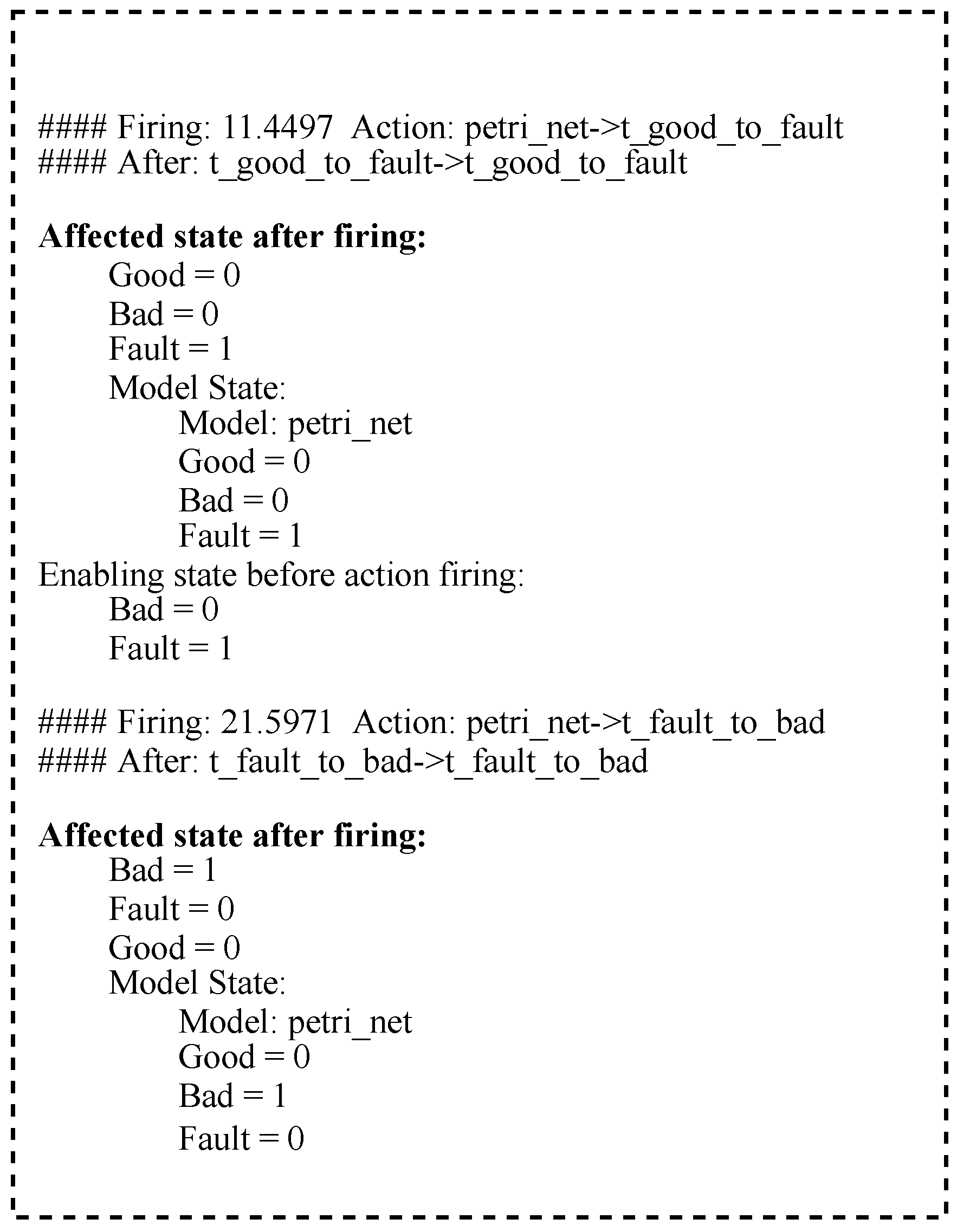
As an output of the simulation, the software generates a log text file that records all the actions executed during the simulation, including the network’s current state and all of the transitions fired, together with their firing time. Figure 6 presents an example of the log created by the simulation.

In order to process the log file and create a dataset for training, an algorithm was designed by the authors. The primary objective was to construct a continuous time series that reflects the entire simulation.

The log files produced by Möbius contain critical information about the simulated system. They provide the following details for each epoch:

• State before transition: The network’s state before a transition takes place.
• State after transition: The network’s state after a transition occurs.
• Transition information: Details about the transition itself, including its name or identifier, and the firing time in seconds.
• Affected states: The states that are impacted by the firing of the transition.

These details are recorded for all the epochs simulated, giving a complete account of the system’s behavior throughout the simulation.

The authors leveraged natural language processing (NLP) tools and techniques to process the log files. The goal was to extract pertinent patterns related to each fired transition, including the firing time and network state data. NLP techniques can analyze and extract structured information from textual data, using methods such as text parsing, pattern matching, and even machine learning models. In this case, however, applying machine learning models for file processing was unnecessary.

As the log file only contains information about discrete transition firing times, a time step concept was introduced to transform it into a continuous time series. This involved calculating the time intervals between all the network transitions within a particular data batch. Among all these intervals, the one with the shortest duration was used as the basis for defining the time step. Thus, for better representing the sign, it was opted to set the time step as half of the minimum interval, in accordance with the Nyquist theorem [38].

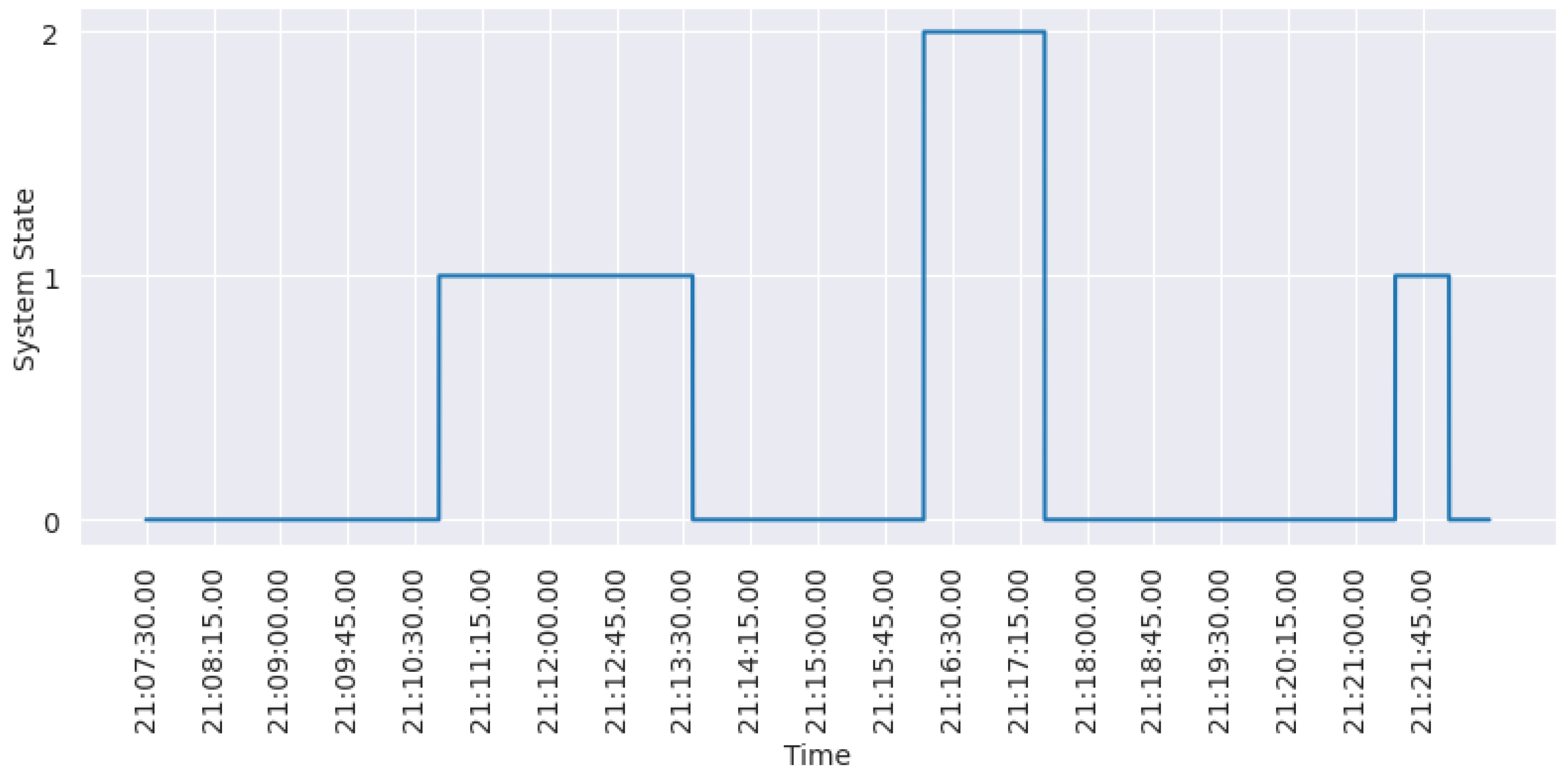
For this study, five simulation batches were utilized. In each batch, the time step was computed following the aforementioned criteria, and the final time step was determined as the shortest among them. Figure 7 shows the behavior of the time series generated in this study for System 2. Levels 0, 1, and 2 on the y-axis represent, respectively, the system states: Good, Fault, and Bad.

The concept of the time step was introduced to fill in the gaps between the recorded transition firings in the log. By employing a consistent time step value, the authors could create a continuous time series that more accurately captured the system’s behavior. This approach yielded a smoother representation of the system dynamics and facilitated additional analysis and modeling.

The first system depicted the two states, Bad and Good, using binary classes. Class 1 was assigned to the Bad state, while class 0 represented the Good state. In the second system, the three states Good, Fault, and Bad were represented by three class labels: 0, 1, and 2, respectively. This was performed to produce already encoded features. When learning the first system, the SNN model will perform binary classification on the time series, whereas for the second system, a multi-class problem is set.

To create the dataset for model training, the authors generated features by lagging the time series data. Specifically, four lagged time series features were created based on the previous samples in time: $t-1$, $t-2$, $t-3$, and $t-4$, where t represents the time instance. The model’s target was set as the system state at time t. This approach allows the model to learn the relationship between the lagged time series features and the current system state, enabling it to make predictions based on historical patterns.

3.2. Model Training

In this study, the authors employed the NengoDL framework to train their spiking neural network (SNN) model. NengoDL facilitated both the simulation and optimization of the SNN, offering the advantage of defining the network architecture similarly to conventional ANNs. This flexibility allowed the authors to set up the network architecture in a manner similar to how they would with TensorFlow, simplifying the process of designing and training the SNN model.

Furthermore, NengoDL facilitated the training process using conventional backpropagation. This was achievable through the utilization of a differentiable function, known as SoftLIF [39], which serves as an approximation of the non-differentiable original function in the LIF (leaky integrate-and-fire) model. By incorporating this approximation, the tool enables the seamless integration of gradients during training, making it feasible to apply standard backpropagation techniques to optimize spiking neural networks. To optimize the model, the Adam method was used, which is a popular algorithm for performing stochastic gradient descent (SGD) [40].

During the testing phase, the trained model takes the input data and simulates them repeatedly over multiple time steps. This repetition of the input data over time is performed to capture the spiking activity of the neurons in response to the input stimulus. For each step, the model generates a response for the neurons in the output layer. To determine the predicted class for a given input, the authors considered the neuron that exhibited the highest mean firing rate across all the simulation steps the winner.

Data Split

In this research, the authors divided the training dataset for the spiking neural network (SNN) into train and test sets, with the test set comprising 20% of the data. Considering the experiment’s focus on time series analysis, a distinctive approach was taken for data division. The dataset was left unshuffled, and the final 20% of the data, representing the latest periods, was designated as the test set. By retaining the chronological order of the data and selecting the final 20% as the test set, the authors aimed to evaluate the performance of the trained SNN models on unseen future data. This approach reflects the time-dependent nature of the problem, allowing the models to be tested on data that closely resemble real-world scenarios.

In the context of the experiment, the time series that were generated for the experiment, the data percentage distributions of the states are shown as follows: Concerning System 1, the training set demonstrates a distribution with 64.72% of the Good state (operational) and 35.28% of the Bad state (nonoperational). The test set comprises 67.24% in the Good state and 32.76% in the Bad state. For System 2, the data showcase a distribution of 87.38% of the Good state, 9.47% of the Fault state (damaged but still operational), and 3.15% of the Bad state (nonoperational) category, whereas the test set encompasses 87.36% in the Good state, 9.95% of the Fault state and 2.69% of the Bad state.

3.3. Hyperparameterization and Architecture of the Networks

In light of its simplicity and computational efficiency, the leaky integrate-and-fire (LIF) neuron model was chosen for all network layers. Thus, the hyperparameterization task focused on finding an optimal set of parameters for the LIF neuron model. These parameters include the following:

• Refractory time constant (${\tau }_{\mathrm{ref}}$): This parameter specifies the duration of the neuron’s rest or refractory period following the firing of a spike.
• Membrane time constant (${\tau }_{\mathrm{rc}}$): This parameter dictates the rate at which the neuron’s membrane potential changes over time.
• Amplitude: In the Nengo framework, the amplitude parameter modulates the intensity of the input given to the neuron.
• Minimum voltage: This parameter establishes the minimum voltage threshold for the neuron.

In addition to these neuron-specific parameters, the authors also optimized other aspects of the SNN models. This includes determining the appropriate number of steps for the simulation, which affects the temporal resolution and accuracy of the model’s predictions. The learning rate of the algorithm used to train the SNN models was also optimized to ensure efficient learning and convergence. Regarding the LSTMs, the authors set conventional training parameters, such as the learning rate, exponential rate decay for the 1st momentum ($beta\_1$), and exponential decay for the 2nd momentum ($beta\_2$). To achieve the set of best parameters, a grid search was performed, exploring a range of distinct values for these parameters. The model’s architecture for each system was defined as follows:

• System 1 (two states).

  –

  First layer: An input layer, of the dense type, with four neurons.

  –

  Second layer: A dense layer with 15 LIF neurons.

  –

  Third layer: An output layer, of the dense type, with two LIF neurons.

• System 2 (three states)

  –

  First layer: An input layer, of the dense type, with four neurons.

  –

  Second layer: A dense layer with 15 LIF neurons.

  –

  Third layer: A dense layer with 15 LIF neurons

  –

  Fourth layer: A dense layer with 15 LIF neurons

  –

  Fifth layer: An output layer, of the dense type, composed of three LIF neurons.

The LSTM networks followed a similar architecture but with conventional neuron models instead. Its architectures were defined as follows:

• System 1 (two states).

  –

  First layer: An input LSTM layer, with four neurons.

  –

  Second layer: A dense layer with 15 neurons.

  –

  Third layer: An output layer, of the dense type, with two LIF neurons.

• System 2 (three states).

  –

  First layer: An input LSTM layer with four neurons.

  –

  Second layer: A LSTM layer with 15 neurons.

  –

  Third layer: A LSTM layer with 15 neurons.

  –

  Fourth layer: A LSTM layer, of the dense type, with 15 neurons.

  –

  Fifth layer: An output layer, of the dense type, composed of three neurons.

In both models, each dense layer’s weights were initialized using the HeNormal method [41], and the softmax activation function was applied to the last layer.

For executing the grid search of parameters, the authors employed weights and biases (WandB) [42], a suite of machine learning experiment tracking tools. WandB enables users to log and track various aspects of the experiment, including hyperparameters, metrics, and visualizations. It provides a convenient interface for organizing and comparing different experiments, making it easier to analyze and interpret the results. Consequently, the experiment could be tracked, with the classification performance measured by accuracy, recall, and F2-score statistical metrics.

4. Results

This section outlines the results for the two systems previously discussed. The first system consists of two states, Good and Bad, while the second system comprises three states, Good, Fault, and Bad. A description of potential transitions for each system is provided below to enhance the understanding of their dynamics.

• System 1.

  –

  Good to Bad—this transition signifies a complete halt in the system due to a failure.

  –

  Bad to Good—this transition signifies a complete recovery of the system after a specific failure.

• System 2.

  –

  Good to Fault—this indicates that a failure has occurred, but the system continues to operate.

  –

  Fault to Bad—this signifies a critical failure, leading the system, already impaired, to halt entirely.

  –

  Bad to Fault—This indicates partial system repair, even though the system remains impaired.

  –

  Good to Bad—This signifies a complete system stoppage due to a critical failure.

  –

  Bad to Good—This indicates a full system recovery following a prior critical failure.

These transitions capture the different states and behaviors of each system, including failures, repairs, and system stoppages. The settings used in the simulation of the Petri networks are shown in Table 1 and Table 2, respectively.

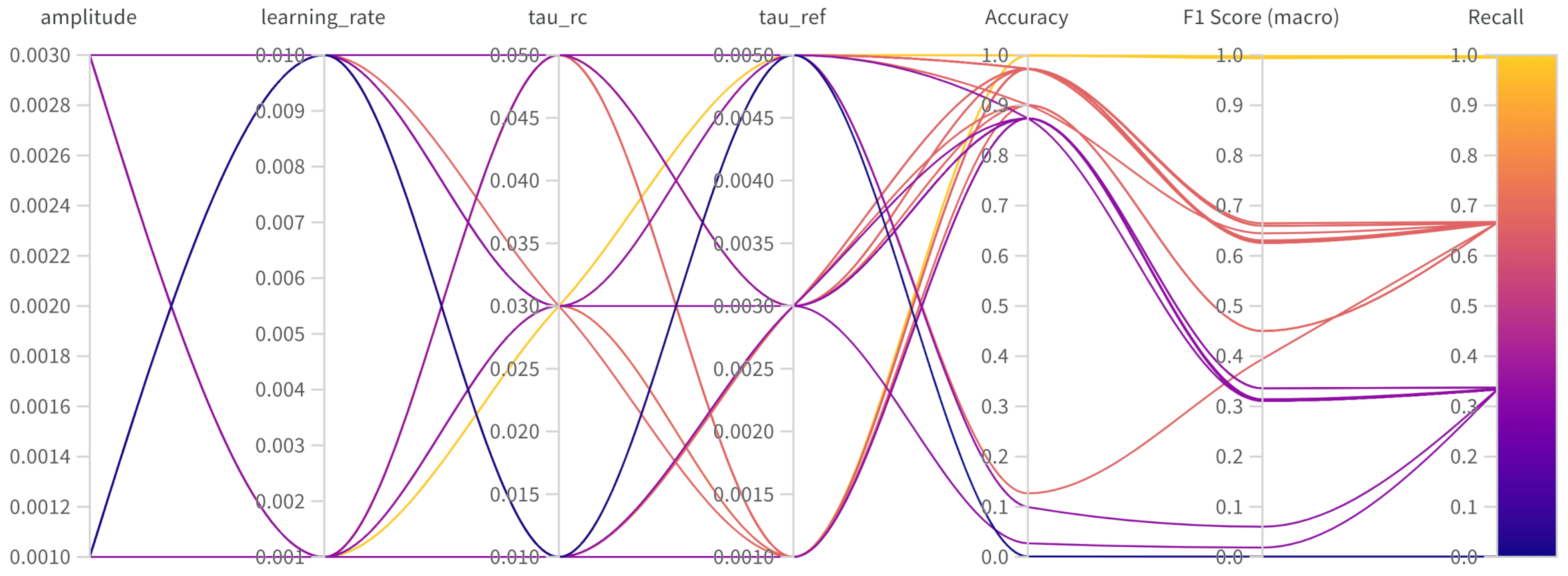
For a visual understanding of the results obtained in this experiment, Figure 8 shows a parallel coordinates chart produced by the grid search for the network associated with System 2. In this chart, each line represents a specific configuration from the grid search and its respective results for the metrics.

The parameterization that yielded improved performance for the spiking neural network models of Systems 1 and 2 are shown in

Table 3. Parameterizion of SNN models.

SNN	Amplitude	${\mathit{\tau }}_{\mathit{rc}}$	${\mathit{\tau }}_{\mathit{ref}}$	Learning Rate
System 1	0.003	0.03	0.003	0.001
System 2	0.001	0.03	0.005	0.001

. These parameter values were found to yield superior results in terms of the model’s performance during the training and testing phases. Similarly, the LSTM models were trained using the Adam algorithm with the following parameter settings: learning rate—0.001; $beta\_1$ (exponential rate decay for 1st moment)—0.09; and $beta\_2$ (exponential rate decay for 2nd moment)—0.999.

Table 4. SNN and LSTM metrics for the two-stage system.

	Accuracy	Recall	F1-Score
SNN	0.99	0.99	0.99
LSTM	0.99	0.99	0.99

and

Table 5. SNN and LSTM metrics for the three-stage system.

	Accuracy	Recall	F1-Score
SNN	0.99	0.99	0.99
LSTM	0.99	0.98	0.98

present the complete set of metrics obtained from the SNN trained to predict the fault classes for both Systems 1 and 2, respectively. These tables also include a comparative analysis with LSTM results, with the models compared in terms of accuracy, recall, and F1-score.

From these findings, it is evident that both SNN and LSTM demonstrated strong performance in terms of accuracy and F1-score for both systems. As mentioned before, this study also evaluated the proposed SNN in three different scenarios, each characterized by a different frequency of severe faults. These scenarios are as follows:

• A severe fault every six months.
• A severe fault each year.
• A severe fault every two years.

It is important to note that the trained SNN models were not retrained specifically for predicting in these new scenarios. This approach was adopted to assess the robustness of the SNN in the face of data drift. The results of the evaluation can be found in

Table 6. Model results when applying a severe failure to the system.

Failure Frequency	Model	Accuracy	Recall	F1-Score
Six months	SNN	0.99	0.99	0.99
	LSTM	0.99	0.99	0.99
1 year	SNN	0.99	0.99	0.99
	LSTM	0.98	0.98	0.98
2 years	SNN	0.99	0.99	0.99
	LSTM	0.98	0.98	0.98

. Overall, both the LSTM model and the SNN model demonstrated robustness and consistency in predicting the system behavior, when handling severe faults over time.

5. Conclusions

Based on the experiments conducted in this work, it can be concluded that the proposed SNN models, along with the LSTM models, show promising results for predicting system behavior in the context of fault detection and classification. The use of stochastic Petri nets (SPNs) as a modeling approach was shown to be an effective approach to reproduce the system behaviors, in scenarios of fault, in a concise and reliable manner.

The SNN models delivered high accuracy and strong performance for recall and F1-score, thus demonstrating their proficiency in accurately classifying system states and identifying faults. When compared to LSTM models, the performance of both methodologies was similar, suggesting that either approach could be efficiently applied to the task at hand.

The evaluation of the SNN models in different scenarios, including data drift, demonstrated their robustness and generalization capabilities. The model was able to handle different fault frequencies without retraining, providing reliable predictions, even in scenarios not encountered during training. This highlights the adaptability and versatility of the SNN models.

The use of Nengo and NengoDL frameworks enabled the efficient simulation and training of the SNN models, while the grid search approach facilitated the tuning of hyperparameters for the LIF neuron model. The SNN models also showed potential to be implemented in neuromorphic hardware with low energy consumption, which can be a good benefit for implementing it into embedded systems, making it possible to perform real-time fault detection and classification without relying on cloud-based or computationally costly solutions.

Looking forward, future work in the field of SNNs could focus on in-depth research into learning algorithms explicitly designed for SNNs. This pursuit aims to boost the performance of SNNs by taking into account the unique traits of spiking neural networks, such as spike-timing dynamics and temporal encoding. Moreover, investigating other network architectures for SNNs, including the exploration of diverse neuron models, connectivity patterns, and layer structures, could further enhance their performance and capabilities. With respect to the context of data generation, the authors intend to include real-world datasets so that external factors can be incorporated into the analysis, such as environmental changes, human factors, maintenance practices, vibrations, and machine natural wear, among others. Furthermore, the authors also intend to include other machine learning models, including booster models and deep learning models to enrich the comparison analysis.