
Control Strategy Based on Artificial Intelligence for a Double-Stage Absorption Heat Transformer


Abstract
1. Introduction
2. Materials and Methods
2.1. Absorption Cycle
2.1.1. Single-Stage Heat Transformer (SSHT)
2.1.2. Double-Stage Heat Transformer (DSHT)
- COP can be defined as the heat recovery capacity or the efficiency of transformation of useful heat with respect to the one supplied, as in Equations (1) and (2):
- GTL is defined as the difference between the temperature of the Absorber (TAB) and Evaporator (TEV), as in Equations (3) and (4):
- FR is a dimensionless value that is defined as the ratio between the concentration of the concentrated solution of lithium bromide in the Generator (XGE) divided by the difference in concentrations of concentrated and diluted lithium bromide in the Generator and Absorber (XGE − XAB), respectively, and is equivalent to the ratio between the flow of the dilution solution in lithium bromide with the ratio to the working fluid or refrigerant fluid, as per Equations (5)–(8):
2.2. Artificial Intelligence
- Cp is the heat capacity of the fluid entering the Generator.
- TF is the outlet temperature of the fluid that comes from a heat source after passing through the Generator.
- TGE_S and TEV_S are the temperature of a constant heat source from which energy is entered into the generation and evaporation processes.
- M1_sim: is the flow of a heat source to the Generator (geothermal, solar, industrial waste).
- M2_sim: is the flow of a heat source to the Evaporator (may be the same as the Generator).
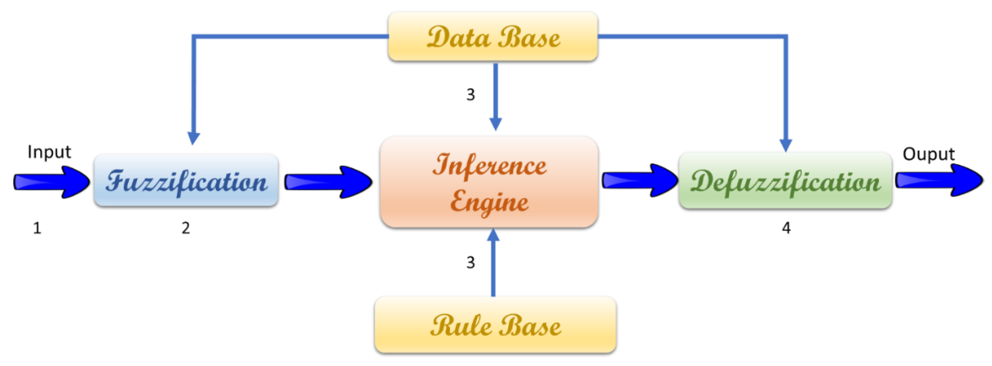
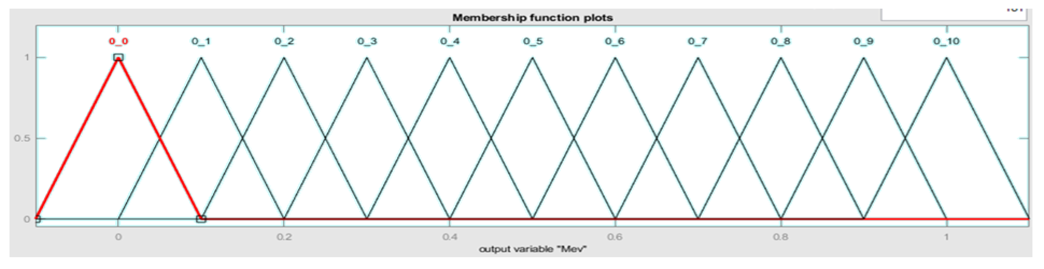
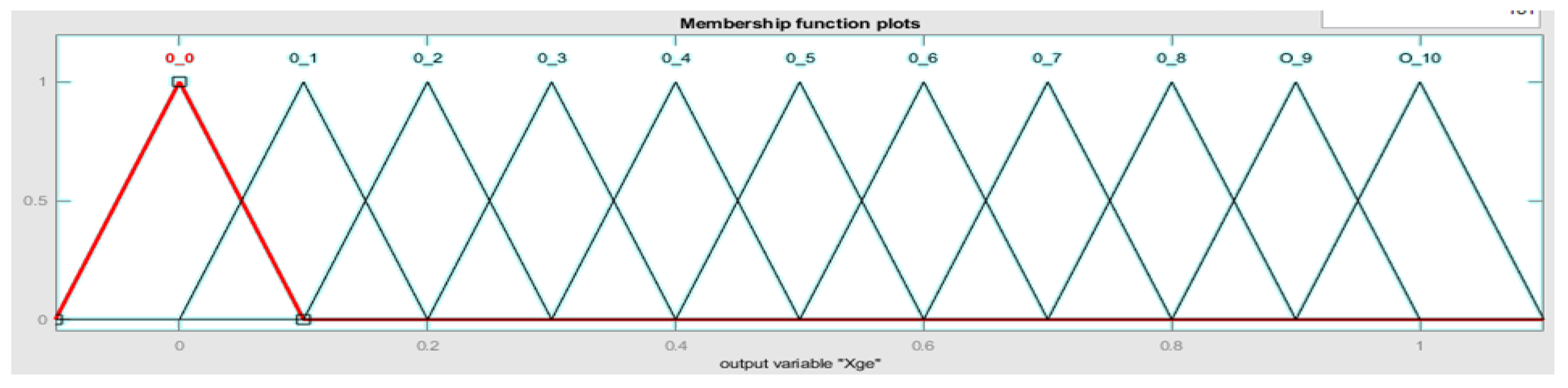
2.2.1. Computational Model Using Fuzzy Logic
- Input variables can be words or sentences, which, through membership functions, are converted into linguistic variables.
- The fuzzification generates a blurred output, that is, the sharp values are blurred for a fuzzy output.
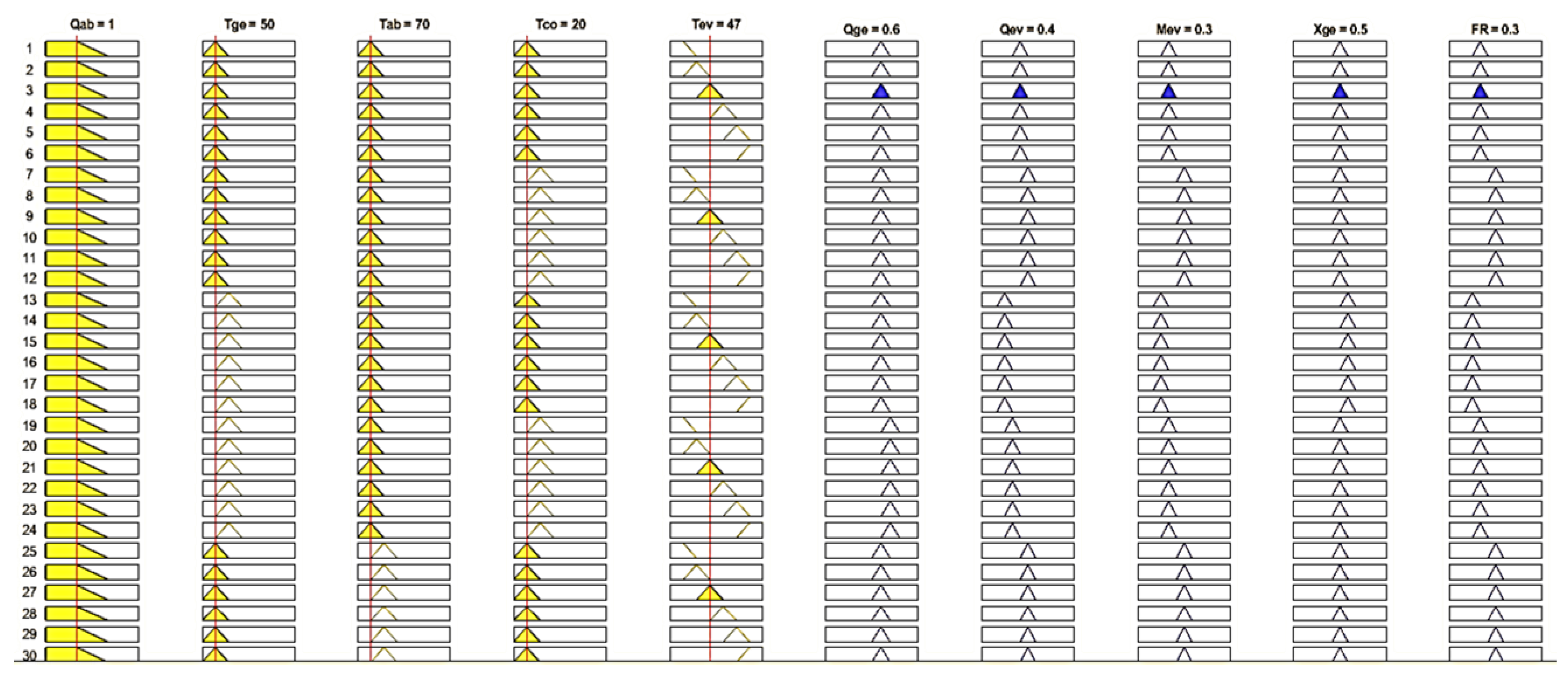
- The mechanisms of fuzzy inference have the task of interpreting the rules of type IF–THEN contained in the rule base of the physical phenomenon to obtain the output values from the current values of the linguistic variables input to the system as indicated by the program.
- Defuzzification is the conversion of a diffuse quantity into a precise quantity. The output of a fuzzy process can be the logical union of two or more fuzzy membership functions defined in the discourse universe of the output variable. Among the methods that have been proposed in the literature to perform the defuzzification stage is the centroid method, which is defined by Equation (11) that determines the defuzzified × value [43]:where:
- n represents the number of items in the sample;
- are the elements;
- is the membership value for point xi in the universe of discourse.
- 1.
- If (QAB is 1) and (TAB is 70) and (TGE is 50) and (Tco is 20) and (TEV is 45) then (QGE is 0_6) (QEV is 0_4) (MEV is 0_3) (XGE is 0_5) (FR is 0_3)
- ...
- 7.
- If (QAB is 1) and (TAB is 70) and (TGE is 50) and (Tco is 21) and (TEV is 45) then (QGE is 0_6) (QEV is 0_5) (MEV is 0_5) (XGE is 0_5) (FR is 0_5)
- ...
- 13.
- If (QAB is 1) and (TAB is 70) and (TGE is 50) and (Tco is 22) and (TEV is 45) then (QGE is 0_6) (QEV is 0_2) (MEV is 0_2) (XGE is 0_5) (FR is 0_6)
- ...
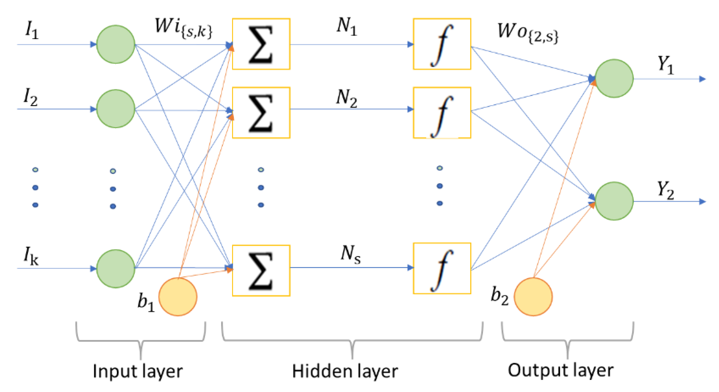
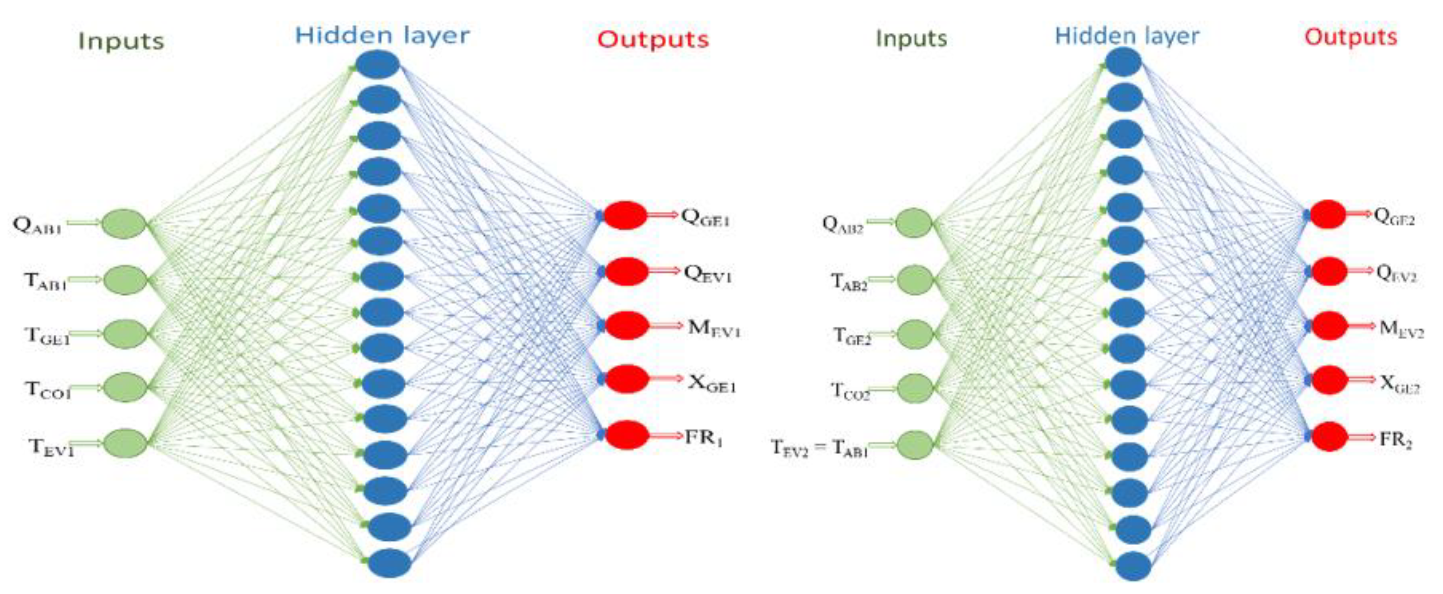
2.2.2. Computational Model using Neural Networks
- A hidden layer (the user can change the number of hidden units).
- Hidden units have a sigmoid activation function (tansig or logsig) while output units have a linear activation function.
- The training algorithm is Backpropagation based on a Levenberg–Marquardt minimization method.
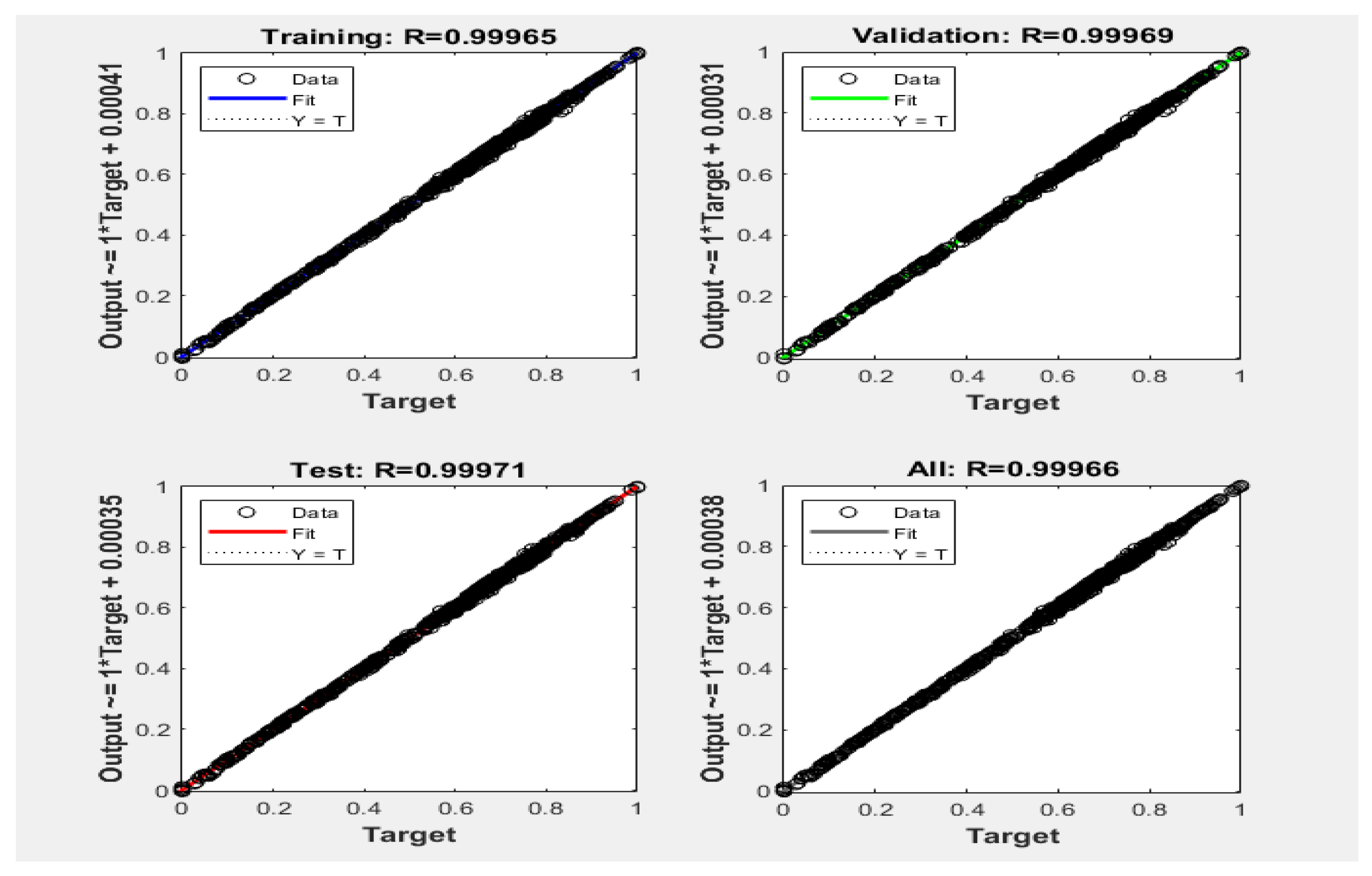
- The learning process is controlled by a cross-validation technique based on a random division of the initial data set into 3 subsets: training (weight adjustment), control of the learning process (validation) and evaluation of the quality of the approach (testing).
- Mean square error (MSE): expresses the difference between the correct outputs and those provided by the network; the approximation is better if MSE is smaller (closer to 0).
- Pearson Correlation Coefficient (R): measures the correlation between correct outputs and those provided by the network; the closer R is to 1, the better the approximation.
2.3. Validation of the Two Models
- Deviation (%): allows you to see how far an approximate value is from an exact one.
- Mean square error root (RMSE): Measures the amount of error that exists between two sets of data, that is, it gives us a measure of how close the points of the observed data are to the estimated values. Near-zero values of RMSE indicate a better fit, and a value of RMSE = 0 indicates a perfect fit between the observed series and the estimated series.
- Mean Error Bias (MBE): Used to validate model results against experimental data, it represents the degree of correspondence between a prediction and an observation, describing whether a model overestimates or underestimates the observation.
- Coefficient of determination (R2) indicates the goodness-of-fit of the model, and its limits are from 0 to 1; 0 indicates that the proposed model does not reproduce the data, and 1 indicates a perfect reproduction of the data entered.
3. Results
3.1. Fuzzy Logic
Fuzzy Logic Output
3.2. Computational Model Based on Neural Networks
3.3. Comparison of Both Computational Models
3.4. ANN for DSHT
4. Discussion
5. Conclusions
Author Contributions
Funding
Conflicts of Interest
References
- IEA. International Energy Agency. Available online: https://www.iea.org/reports/energy-technology-perspectives-2023 (accessed on 6 February 2023).
- IEA. International Energy Agency World Energy Outlook. 2022. Available online: https://www.iea.org/reports/world-energy-outlook-2022 (accessed on 9 December 2022).
- Oyepedo, S.O.; Fakeye, B.A. Waste heat recovery technologies: Pathway to sustainable energy development. J. Therm. Eng. 2021, 7, 324–348. [Google Scholar]
- Romero, R.J.; Cerezo, J.; Rodriguez-Martinez, A.; Montiel, M. Absorption Heat Transformer for Solar Pond Energy Temperature Upgrading. Chem. Eng. Trans. 2021, 86, 703–708. [Google Scholar]
- Wang, H.; Li, H.; Wang, L.; Bu, X.; Zeng, J.; Xie, N.; Xu, Q. A solar-assisted double absorption heat transformer: Off-design performance and optimum control strategy. Energy Convers. Manag. 2019, 196, 614–622. [Google Scholar] [CrossRef]
- Cudok, F.; Giannetti, N.; Ciganda, J.L.C.; Aoyama, J.; Babu, P.; Coronas, A.; Ziegler, F. Absorption heat transformer-state-of-the-art of industrial applications. Renew. Sustain. Energy Rev. 2021, 141, 110757. [Google Scholar] [CrossRef]
- Yari, M.; Salehi, S.; Mahmoudi, S.M.S. Three-objective optimization of water desalination systems based on the double-stage absorption heat transformers. Desalination 2017, 405, 10–28. [Google Scholar] [CrossRef]
- Huicochea, A.; Siqueiros, J.; Romero, R.J. Portable water purification system integrated to a heat transformer. Desalination 2004, 165, 385–391. [Google Scholar] [CrossRef]
- Huicochea, A.; Siqueiros, J. Increase of COP for an experimental heat transformer using a water purification system. Desalination Water Treat 2009, 12, 305–312. [Google Scholar] [CrossRef]
- Huicochea, A.; Siqueiros, J. Improved efficiency of energy use of a heat transformer using a water purification system. Desalination 2010, 257, 8–15. [Google Scholar] [CrossRef]
- Rivera, W.; Huicochea, A.; Martínez, H.; Siqueiros, J.; Juarez, D.; Cadenas, E. Exergy analysis of an experimental heat transformer for water purification. Energy 2011, 36, 320–327. [Google Scholar] [CrossRef]
- Sekar, S.; Saravanan, R. Experimental studies on absorption heat transformer coupled distillation system. Desalination 2011, 274, 292–301. [Google Scholar] [CrossRef]
- Huicochea, A.; Rivera, W.; Martínez, H.; Siqueiros, J.; Cadenas, E. Analysis of the behavior of an experimental absorption heat transformer for water purification for different mass flux rates in the generator. Appl. Therm. Eng. 2013, 52, 38–45. [Google Scholar] [CrossRef]
- Meza, M.; Marquez-Nolasco, A.; Huicochea, A.; Juarez-Romero, D.; Siqueiros, J. Experimental study of an absorption heat transformer with heat recycling to the generator. Exp. Therm. Fluid Sci. 2014, 53, 171–178. [Google Scholar] [CrossRef]
- Cortés, E.; Rivera, W. Exergetic and exergoeconomic optimization of a cogeneration pulp and paper mill plant including the use of a heat transformer. Energy 2010, 35, 1289–1299. [Google Scholar] [CrossRef]
- Horus, I.; Kurt, B. Absorption heat transformers and an industrial application. Renew. Energy 2010, 35, 2175–2181. [Google Scholar] [CrossRef]
- Rivera, W.; Best, R.; Cardoso, M.J.; Romero, R.J. A review of absorption heat transformers. Appl. Therm. Eng. 2015, 91, 654–670. [Google Scholar] [CrossRef]
- Romero, R.; Rodriguez-Martinez, A.; Cerezo, J.; Rivera, W. Comparison of Double Stage Heat Transformer with Double Absorption Heat Transformer Operating with Carrol—Water for Industrial Waste Heat Recovery. Chem. Eng. Trans. 2011, 25, 129–134. [Google Scholar]
- Rivera, W.; Cerezo, J.; Rivero, R.; Cervantes, J.; Best, R. Single stage and double absorption heat transformers used to recover energy in a distillation column of butane and pentane. Int. J. Energy Res. 2003, 27, 1279–1292. [Google Scholar] [CrossRef]
- Ma, X.; Chen, J.; Li, S.; Sha, Q.; Liang, A.; Li, W.; Zhang, J.; Zheng, G.; Feng, Z. Application of absorption heat transformer to recover waste heat from a synthetic rubber plant. Appl. Therm. Eng. 2003, 23, 797–806. [Google Scholar] [CrossRef]
- Fujii, T.; Kawamura, H.; Uchida, S.; Nishiguchi, A. A single-effect absorption heat transformer for waste heat recovery in industrial use. In Proceedings of the 9th International IEA Heat Pump Conference, Zürich, Switzerland, 20–22 May 2008; Conference Proceedings Paper. International Energy Agency: Paris, France, 2008. [Google Scholar]
- Fujii, T.; Uchida, S.; Nishiguchi, A. Development Activities of Low Temperature Waste Heat Recovery Appliances using Absorption Heat Pumps. In Proceedings of the International Symposium on Next-Generation Air Conditioning and Refrigeration Technology, Tokyo, Japan, 17–19 February 2010. [Google Scholar]
- Parham, K.; Khamooshi, M.; Daneshvar, S.; Assadi, M.; Yari, M. Comparative assessment of different categories of absorption heat transformers in water desalination process. Desalination 2016, 396, 17–29. [Google Scholar] [CrossRef]
- Vázquez-Aveledo, S.; Diaz-Gonzalez, L.; Montiel-Gonzalez, M.; Romero, R.J. Risk of Overwarming for Flow Variation into an Absorption Heat Transformer for Waste Heat Recovery Process. Chem. Eng. Trans. 2022, 91, 373–378. [Google Scholar]
- Rivera, W.; Romero, R.; Cardoso, M.J.; Aguillón, J.; Best, R. Theoretical and experimental comparison of the performance of a single-stage heat transformer operating with water/lithium bromide and water/Carrol. Int. J. Energy Res. 2002, 26, 747–762. [Google Scholar] [CrossRef]
- Hdz-Jasso, A.M.; Contreras-Valenzuela, M.R.; Rodríguez-Martínez, A.; Romero, R.J.; Venegas, M. Experimental heat transformer monitoring based on linear modelling and statistical control process. Appl. Therm. Eng. 2015, 75, 1271–1286. [Google Scholar] [CrossRef]
- Goyal, A.; Staedter, M.A.; Garimella, S. A review of control methodologies for vapor compression and absorption heat pumps. Int. J. Refrig. Rev. Int. Du Froid 2018, 97, 1–20. [Google Scholar] [CrossRef]
- Broersen, P.M.T.; Van Der Jagt, M.F.G. Hunting of Evaporators Controlled by a Thermostatic Expansion Valve. J. Dyn. Syst. Meas. Control. 1980, 102, 130–135. [Google Scholar] [CrossRef]
- Gruhle, W.D.; Isermann, R. Modeling and Control of a Refrigerant Evaporator. J. Dyn. Syst. Meas. Control. 1985, 107, 235–240. [Google Scholar] [CrossRef]
- Qureshi, T.Q.; Tassou, S.A. Variable-Speed Capacity Control in Refrigeration Systems. Appl. Therm. Eng. 1996, 16, 103–113. [Google Scholar] [CrossRef]
- Marcinichen, J.B.; Holanda, T.N.D.; Melo, C.A. Dual Siso Controller for a Vapor Compression Refrigeration System. In Proceedings of the International Refrigeration and Air-Conditioning Conference, West Lafayette, IN, USA, 14–17 July 2008. [Google Scholar]
- Li, X.; Chen, J.; Chen, Z.; Liu, W.; Hu, W.; Liu, X. A New Method for Controlling Refrigerant Flow in Automobile Air Conditioning. Appl. Therm. Eng. 2004, 24, 1073–1085. [Google Scholar] [CrossRef]
- Ekren, O.; Sahin, S.; Isler, Y. Comparison of Different Controllers for Variable Speed Compressor and Electronic Expansion Valve. Int. J. Refrig. 2010, 33, 1161–1168. [Google Scholar] [CrossRef]
- Rêgo, A.T.; Hanriot, S.M.; Oliveira, A.F.; Brito, P.; Rêgo, T.F.U. Automotive Exhaust Gas Flow Control for an Ammonia–Water Absorption Refrigeration System. Appl. Therm. Eng. 2014, 64, 101–107. [Google Scholar] [CrossRef]
- Goyal, A.; Rattner, A.S.; Garimella, S. Model-Based Feedback Control of an Ammonia-Water Absorption Chiller. Sci. Technol. Built Environ. 2015, 21, 357–364. [Google Scholar] [CrossRef]
- Zinet, M.; Rulliere, R.; Haberschill, A. Numerical Model for the Dynamic Simulation of a Recirculation Single-Effect Absorption Chiller. Energy Convers. Manag. 2012, 62, 51–63. [Google Scholar] [CrossRef]
- Xu, Y.J.; Zhang, S.J.; Xiao, Y. Modeling the Dynamic Simulation and Control of a Single Effect H2O-Libr Absorption Chiller. Appl. Therm. Eng. 2016, 107, 1183–1191. [Google Scholar] [CrossRef]
- Garcíadealva, Y.; Best, R.; Hugo, H.; Vargas, A.; Rivera, W.; Jiménez-García, J.C. A Cascade Proportional Integral Derivative Control for a Plate-Heat-Exchanger-Based Solar Absorption Cooling System. Energies 2021, 14, 4058. [Google Scholar] [CrossRef]
- Silva-Sotelo, S.; Romero, R.; Rodríguez-Martínez, A. Double Stage Heat Transformer Controlled by Flow Ratio. In Innovations in Computing Sciences and Software Engineering; Springer: Dordrecht, The Netherlands, 2009; pp. 577–581. [Google Scholar]
- Santos, M. Un enfoque aplicado al control inteligente. Rev. Iberoam. De Automática E Inf. Ind. 2011, 8, 283–296. [Google Scholar] [CrossRef]
- Valdez, V.; Romero, R. Optimal Design Criterion for Heat Transformer operating with Water Carrol. In Proceedings of the International Conference on Advanced in Mechanical and Atomation Engineering-MAE2016, Rome, Italy, 18–19 August 2016; SEEK Digital Library: New York, NY, USA, 2016; pp. 57–59. [Google Scholar]
- Belman-Flores, J.M.; Rodríguez-Valderrama, D.A.; Ledesma, S.; García-Pabón, J.J.; Hernández, D.; Pardo-Cely, D.M. A Review on Applications of Fuzzy Logic Control for Refrigeration Systems. Appl. Sci. 2022, 12, 1302. [Google Scholar] [CrossRef]
- Islam, M.A.; Hossain, M.S.; Haque, I.S.M. Mathematical Comparison of Defuzzification of Fuzzy Logic Controller for Intelligence Air Conditioning System. Int. J. Sci. Res. Math. Stat. Sci. 2021, 8, 29–37. [Google Scholar]
- MathWork. Available online: https://es.mathworks.com/products/deep-learning.html (accessed on 17 March 2023).
- Hooda, D.S.; Raich, V. Fuzzy Logic Models and Fuzzy Control an Introduction; Alpha Science International Ltd.: Oxford, UK, 2017; 408p. [Google Scholar]
- Chandwani, V.; Agrawal, V.; Nagar, R. Modeling slump of ready mix concrete using genetic algorithms assisted training of Artificial Neural Networks. Expert Syst. Appl. 2015, 42, 885–893. [Google Scholar] [CrossRef]
- Adil, O.; Ali, M.; Ali, A. Comparison between the Effects of Different Types of Membership Functions on Fuzzy Logic Controller Performance. Int. J. Emerg. Eng. Res. Technol. 2015, 3, 76–83. [Google Scholar]
- Asanza, W.R.; Olivo, B.M. Redes Neuronales Artificiales Aplicadas al Reconocimiento de Patrones; UTMACH: Machala, Ecuador, 2018; pp. 11–35. [Google Scholar]
- Villada, F.; Munoz, N.; García-Quintero, E. Redes Neuronales Artificiales aplicadas a la Predicción del Precio del Oro. Inf. Tecnol. 2016, 27, 143–150. [Google Scholar] [CrossRef]
- Sayed, B.T.; Al-Mohair, H.K.; Alkhayyat, A.; Ramírez-Coronel, A.A.; Elsahabi, M. Comparing machine-learning-based black box techniques and white box models to predict rainfall-runoff in a northern area of Iraq, the Little Khabur River. Water Sci. Technol. 2023, 87, 812–822. [Google Scholar] [CrossRef]
- Farzaneh-Gord, M.; Rahbari, H.R.; Mohseni-Gharesafa, B.; Toikka, A.; Zvereva, I. Accurate determination of natural gas compressibility factor by measuring temperature, pressure and Joule-Thomson coefficient: Artificial neural network approach. J. Pet. Sci. Eng. 2021, 202, 108427. [Google Scholar] [CrossRef]
- Lugo, S.; Morales, L.I.; Best, R.; Gómez, V.H.; García-Valladares, O. Numerical simulation and experimental validation of an outdoor-swimming pool solar heating system in warm climates. Sol. Energy 2019, 189, 45–56. [Google Scholar] [CrossRef]
- Rivera, W.; Romero, R.J.; Cardoso, M.J. Theoretical comparison of single stage and advanced absorption heat transformers operating with water/lithium bromide and water/carrol mixtures. Int. J. Energy Res. 1998, 22, 427–442. [Google Scholar] [CrossRef]
- Hernández, J.A.; Romero, R.J.; Juárez, D.; Escobar, R.F.; Siqueiros, J. A neural network approach and thermodynamic model of waste energy recovery in a heat transformer in a water purification process. Desalination 2009, 243, 273–285. [Google Scholar] [CrossRef]


| Tickets | Outputs |
|---|---|
| QAB: Thermal power of the Absorber [kW] TAB: Absorber temperature [°C] TGE: Generator temperature [°C] TCO: Condenser temperature [°C] TEV: Evaporator temperature [°C] | QGE: Thermal power of the Generator [kW] QEV: Evaporator thermal power [kW] MEV: Working fluid flow [kg/s] XGE: Generator concentration [%w] FR: Flow ratio [Dimensionless] |
| Title 1 | Variables | Universe of Discourse | Language Tags |
|---|---|---|---|
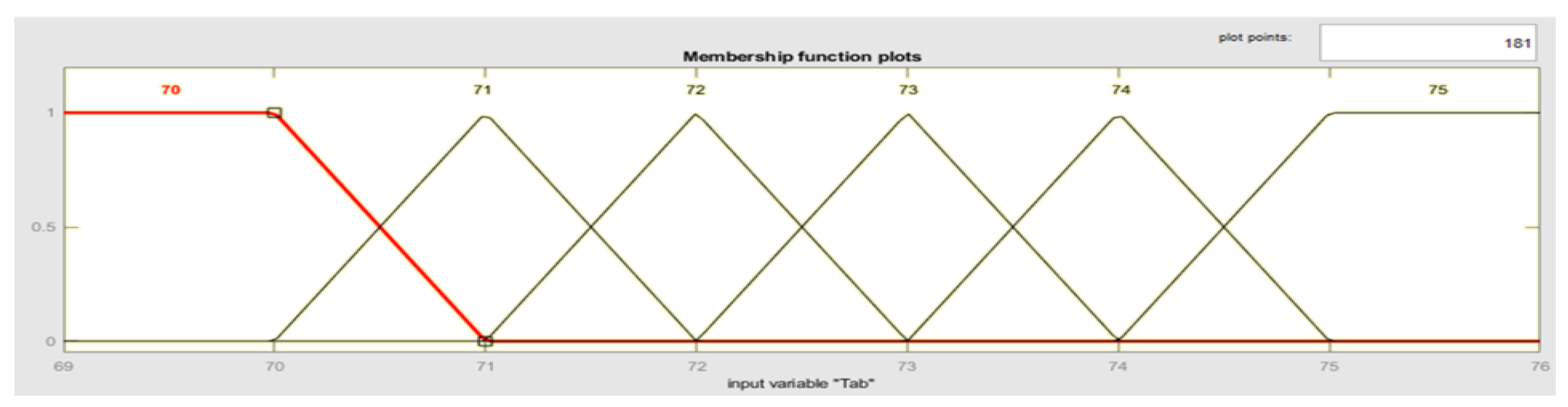
| Tickets | QAB [kW] TCO [°C] TAB [°C] TGE [°C] TEV [°C] | 1–2 20–25 70–75 50–55 45–50 | [1-2] [20-21-22-23-24-25] [70-71-72-73-74-75] [50-51-52-53-54-55] [45-46-47-48-49-50] |
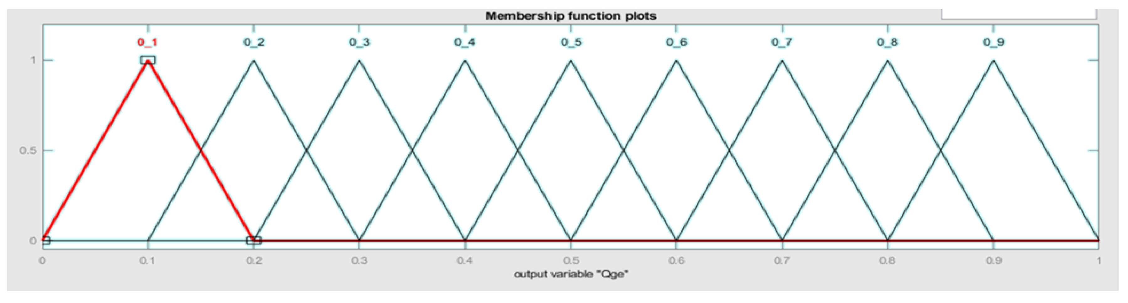
| Outputs | QGE [kW] QEV [kW] MEV [kg/s] XGE [%w] FR [dimensionless] | 0–1 0–1 0–1 0–1 0–1 | [0_0-0_1-0_2-0_3-0_4-0_5-0_6-0_7-0_8-0_9] [0_0-0_1-0_2-0_3-0_4-0_5-0_6-0_7-0_8-0_9] [0_0-0_1-0_2-0_3-0_4-0_5-0_6-0_7-0_8-0_9] [0_0-0_1-0_2-0_3-0_4-0_5-0_6-0_7-0_8-0_9] [0_0-0_1-0_2-0_3-0_4-0_5-0_6-0_7-0_8-0_9] |
| Variables | Value | |
|---|---|---|
| Inputs | QAB [kW] TCO [°C] TAB [°C] TGE [°C] TEV [°C] | 1–2 20–25 70–75 50–55 45–50 |
| Outputs | QGE [kW] QEV [kW] MEV [kg/s] XGE [%w] FR [dimensionless] | 0–1 0–1 0–1 0–1 0–1 |
| Wi{15,1} | Wi{15,2} | Wi{15,3} | Wi{15,4} |
|---|---|---|---|
| −0.9772 | 1.0564 | 0.0028 | 0.9100 |
| −0.8625 | 0.9215 | 0.0023 | 0.8501 |
| −1.8420 | 0.0977 | −0.0015 | 0.0508 |
| 0.0659 | −0.0879 | 5.2562 × 10−05 | 0.0005 |
| 2.738 | −0.0891 | 0.0024 | −0.0348 |
| −2.8736 | 2.8472 | −0.0023 | 2.9076 |
| −5.1080 | 4.7151 | 0.0136 | 0.6338 |
| −2.8530 | 2.8258 | −0.0023 | 2.8669 |
| 3.2812 | 0.0902 | −0.0128 | 0.0313 |
| −1.4776 | 1.0950 | 0.0046 | 1.3413 |
| −1.2590 | 1.2930 | −0.0004 | −4.1966 |
| 5.1733 | −3.9671 | 0.0010 | 8.2166 |
| 7.0039 | −4.6306 | 0.0016 | 10.3212 |
| −0.3480 | 0.0873 | 0.00163 | 0.07205 |
| 0.4706 | −0.3563 | 0.0024 | −0.4261 |
| Wo{1,15}T | Wo{2,15}T | Wo{3,15}T | Wo{4,15}T | Wo{5,15}T |
|---|---|---|---|---|
| −0.0617 | −0.3965 | −0.4247 | 0.0330 | −1.7513 |
| 0.3548 | 0.8390 | 0.8682 | −0.0196 | 2.5417 |
| −0.4964 | 0.7147 | 0.6889 | −0.2471 | 1.3084 |
| 0.4323 | 1.4499 | 1.1029 | 6.3634 | −0.2043 |
| −0.3122 | 0.5054 | 0.4899 | −0.1723 | 0.9649 |
| 0.6374 | 1.1215 | 1.1160 | −0.0060 | 1.3384 |
| −0.0093 | −0.0277 | −0.0276 | 0.0089 | −0.0331 |
| −0.5772 | −0.9895 | −0.9849 | 0.0087 | −1.1827 |
| −0.0203 | 0.0717 | 0.0704 | −0.0282 | 0.1246 |
| −0.0419 | 0.0776 | 0.0724 | −0.0026 | −0.1485 |
| 0.6938 | 1.9976 | 1.9828 | −0.0212 | 2.0050 |
| 0.9950 | 2.9670 | 2.9479 | −0.0706 | 2.9920 |
| −0.8368 | −2.5002 | −2.4841 | 0.0658 | −2.5215 |
| −1.3667 | 0.6120 | 0.5176 | −0.4386 | −0.1777 |
| 0.7445 | −0.2982 | −0.2779 | −0.2779 | 0.3307 |
| b1 | b2 |
|---|---|
| 1.4210 | −0.5270 |
| 1.2001 | 1.3199 |
| 1.3380 | 1.3343 |
| 0.2503 | −1.7314 |
| −1.8645 | 0.6977 |
| 0.8053 | |
| −0.4996 | |
| 0.5853 | |
| −0.0174 | |
| 0.1084 | |
| −7.3954 | |
| 14.8259 | |
| 18.5230 | |
| −0.7086 | |
| 0.7127 |
| Fuzzy Logic | % Dev (max) | RMSE | MBE | R2 |
|---|---|---|---|---|
| QGE | 0.145456403 | 4.20 × 10−04 | 1.76 × 10−07 | 0.974810 |
| QEV | 1.755065786 | 1.21 × 10−02 | 1.45 × 10−04 | 0.984409 |
| MEV | 1.830934034 | 4.81 × 10−06 | 2.32 × 10⁻¹¹ | 0.984793 |
| XGE | 1.008901078 | 1.39 × 10−01 | 1.93 × 10−02 | 0.989974 |
| FR | 6.665546516 | 3.36 × 10−01 | 1.13 × 10−01 | 0.977917 |
| Neural Networks | % Dev (max) | RMSE | MBE | R2 |
| QGE | 0.014784 | 3.10 × 10−05 | 9.61 × 10⁻¹⁰ | 0.99986541 |
| QEV | 0.754447 | 2.94 × 10−03 | 8.66 × 10−06 | 0.99903313 |
| MEV | 0.758600 | 1.18 × 10−06 | 1.39 × 10⁻¹² | 0.99903697 |
| XGE | 0.087526 | 0.18 × 10−01 | 0.03 × 10−02 | 0.99981534 |
| FR | 1.749315 | 0.80 × 10−01 | 1.64 × 10−02 | 0.99872625 |
| Wi{15,1} | Wi{15,2} | Wi{15,3} | Wi{15,4} |
|---|---|---|---|
| 1.2254 | −1.1448 | 0.0041 | −1.1835 |
| −0.2686 | 0.1965 | −0.0033 | 0.2173 |
| −0.0985 | 0.1185 | 0.0011 | −0.0361 |
| 3.6820 | −3.7613 | 0.0221 | −3.2992 |
| 8.8366 | −8.2592 | 0.0008 | −1.8098 |
| 8.7259 | −4.7289 | 0.0029 | −13.2845 |
| −7.8608 | 7.3009 | −0.0025 | 1.11581 |
| −8.4505 | 4.6515 | −0.0014 | 11.6971 |
| 0.1140 | 0.2041 | −0.0012 | −0.1426 |
| 5.4186 | −6.5799 | −0.0012 | 0.9792 |
| 4.1579 | −4.1439 | −0.0180 | −4.2200 |
| −0.6326 | 1.4982 | 9.2773 × 10−05 | −0.8332 |
| −6.6486 | 7.8499 | 0.0007 | −0.9245 |
| 3.4092 | 2.0946 | −0.0843 | −2.9217 |
| −0.2114 | 0.4584 | 0.0040 | −0.2386 |
| Wo{1,15}T | Wo{2,15}T | Wo{3,15}T | Wo{4,15}T | Wo{5,15}T |
|---|---|---|---|---|
| −0.0731 | −0.0966 | −0.0981 | 0.0118 | −0.3688 |
| −0.4621 | −0.2239 | −0.2244 | −0.6377 | −0.7501 |
| −3.1999 | 4.5836 | 4.5869 | −3.4430 | 5.6008 |
| 0.0547 | −0.1547 | −0.1556 | 0.0085 | −0.3077 |
| -0.5996 | 1.0522 | 1.0544 | −0.0376 | 1.2139 |
| −2.3424 | 3.7439 | 3.7407 | 0.0026 | 2.8558 |
| −0.6385 | 1.0985 | 1.1005 | −0.0551 | 1.2548 |
| −2.4679 | 3.9277 | 3.9244 | −0.0062 | 3.0078 |
| −0.0151 | 0.7491 | 0.7735 | −0.2024 | 1.2248 |
| −3.2268 | 4.5012 | 4.5002 | −0.0953 | 3.3789 |
| −0.0011 | −0.0656 | −0.0660 | −0.0058 | −0.1561 |
| 0.0925 | −0.1877 | −0.1882 | 0.0196 | −0.2502 |
| −3.1084 | 4.3051 | 4.3041 | −0.0931 | 3.1681 |
| 0.0070 | 0.0088 | 0.0097 | −0.0021 | 0.0165 |
| 0.6520 | −1.2756 | −1.2773 | 0.0292 | −1.6757 |
| b1 | b2 |
|---|---|
| −2.2891 | −0.2966 |
| 0.0377 | 0.7999 |
| −0.1885 | 0.8097 |
| 6.4594 | −0.6725 |
| 12.8104 | 1.3759 |
| 20.5034 | |
| −11.3639 | |
| −18.7434 | |
| −0.3747 | |
| 10.3655 | |
| −3.9339 | |
| −1.1616 | |
| −12.3745 | |
| 3.31736 | |
| 0.3744 |
| Neural Networks | % Error (max) | RMSE | MBE | R2 |
|---|---|---|---|---|
| QGE2 | 0.067516255 | 1.40 × 10−04 | 1.95 × 10−08 | 0.999467773 |
| QEV2 | 4.168673681 | 1.55 × 10−02 | 2.39 × 10−04 | 0.999441275 |
| MEV2 | 4.202766596 | 6.23 × 10−06 | 3.88 × 10⁻¹¹ | 1.000000000 |
| XGE2 | 0.128334019 | 2.32 × 10−02 | 5.39 × 10−04 | 0.999999808 |
| FR2 | 3.983523963 | 1.47 × 10−01 | 2.18 × 10−02 | 0.999712526 |
Disclaimer/Publisher’s Note: The statements, opinions and data contained in all publications are solely those of the individual author(s) and contributor(s) and not of MDPI and/or the editor(s). MDPI and/or the editor(s) disclaim responsibility for any injury to people or property resulting from any ideas, methods, instructions or products referred to in the content. |
© 2023 by the authors. Licensee MDPI, Basel, Switzerland. This article is an open access article distributed under the terms and conditions of the Creative Commons Attribution (CC BY) license (https://creativecommons.org/licenses/by/4.0/).
Share and Cite
Vázquez-Aveledo, S.; Romero, R.J.; Montiel-González, M.; Cerezo, J. Control Strategy Based on Artificial Intelligence for a Double-Stage Absorption Heat Transformer. Processes 2023, 11, 1632. https://doi.org/10.3390/pr11061632
Vázquez-Aveledo S, Romero RJ, Montiel-González M, Cerezo J. Control Strategy Based on Artificial Intelligence for a Double-Stage Absorption Heat Transformer. Processes. 2023; 11(6):1632. https://doi.org/10.3390/pr11061632
Chicago/Turabian StyleVázquez-Aveledo, Suset, Rosenberg J. Romero, Moisés Montiel-González, and Jesús Cerezo. 2023. "Control Strategy Based on Artificial Intelligence for a Double-Stage Absorption Heat Transformer" Processes 11, no. 6: 1632. https://doi.org/10.3390/pr11061632
APA StyleVázquez-Aveledo, S., Romero, R. J., Montiel-González, M., & Cerezo, J. (2023). Control Strategy Based on Artificial Intelligence for a Double-Stage Absorption Heat Transformer. Processes, 11(6), 1632. https://doi.org/10.3390/pr11061632