Article

Signal-to-Image: Rolling Bearing Fault Diagnosis Using ResNet Family Deep-Learning Models

1
College of Energy and Power Engineering, Lanzhou University of Technology, Lanzhou 730050, China
2
School of Intelligent Manufacturing Engineering, Chongqing University of Arts and Sciences, Chongqing 402160, China
3
School of Engineering, Newcastle University, Newcastle upon Tyne NE1 7RU, UK
4
Department of Computing, The Hong Kong Polytechnic University, Hong Kong 999077, China
*
Author to whom correspondence should be addressed.
Processes 2023, 11(5), 1527; https://doi.org/10.3390/pr11051527
Submission received: 8 April 2023 / Revised: 5 May 2023 / Accepted: 12 May 2023 / Published: 17 May 2023

Abstract

:
Rolling element bearings (REBs) are the most frequent cause of machine breakdowns. Traditional methods for fault diagnosis in rolling bearings rely on feature extraction and signal processing techniques. However, these methods can be affected by the complexity of the underlying patterns and the need for expert knowledge during signal analysis. This paper proposes a novel signal-to-image method in which the raw signal data are transformed into 2D images using continuous wavelet transform (CWT). This transformation enhances the features extracted from the raw data, allowing for further analysis and interpretation. Transformed images of both normal and faulty rolling bearings from the Case Western Reserve University (CWRU) dataset were used with deep-learning models from the ResNet family. They can automatically learn and identify patterns in raw vibration signals after continuous wavelet transform is used, eliminating the need for manual feature extraction. To further improve the training results, squeeze-and-excitation networks (SENets) were added to improve the process. By comparing results obtained from several models, we found that SE-ResNet152 has the best performance for REB fault diagnosis.

1. Introduction

In the modern machine-manufacturing industry, rotation machinery accounts for more than 90% of the market [1]. Of all rotation machines, rolling element bearings (REBs) are one of the most circuital components for providing rotation motion [2]. However, because of complex and changing working conditions, including changes in speed and workload, REBs are also the most frequent cause of machine breakdowns [3]. Therefore, monitoring, detecting, and diagnosing REB fault signals is necessary for rotating machinery systems [4]. A rolling bearing fault diagnosis is mainly focused on signal and intelligent diagnoses [5], techniques that use vibration analysis to detect incipient faults in REBs [6].
The signal analysis research domain includes Fourier transform [7], wavelet packet transform [8], dual-tree complex wavelet transform [9], Parsimonious Network based on fuzzy Inference System (PANFIS) [10] and the acoustic signal-based approach [11]. Variation mode decomposition was proposed by [3] Yonggang Xu et al. [12], and the adaptive kurtogram (AK) method detects fault signals in damaged machines. AK can also be applied to a wheelset-bearing system fault diagnosis [13]. In addition, many other algorithms, such as Fast Entrogram [14] and adaptive periodic mode decomposition (APMD) [15] are also used to diagnose rolling bearing faults.
The intelligent diagnosis domain has become a popular research topic in recent years. As increasingly intelligent techniques develop, they are more widely used in related fields. For example, machine learning (ML) can be adapted from the computer vision field to diagnose faults because of its ability to extract features and classify fault types [16,17].
In [18], linear and nonlinear maps are discussed in detail, illustrating the optimal performance of unsupervised and supervised learning for fault detection. Rolling-bearing fault signal systems can be considered as nonlinear dynamic. Support vector machines (SVMs) can also be adapted for fault classifications [19,20,21] and are a kind of supervised method.
Some of these methods can classify and detect faults in rotation machine systems, but they cannot detect fault features directly from original signals but must calculate a massive amount of data in real time, which means it is difficult to meet engineering requirements that involve increasing data sizes. There is much value in investigating fault diagnosis methods that can detect fault features from original signals, perform real-time calculations automatically, and provide health-status feedback.
In recent years, with the development of deep learning (DL), an increasing number of researchers have become interested in using DL methods [16,22] to address the aforementioned problems, and many have been applied to rolling-bearing fault diagnosis. Convolutional neural networks (CNNs) are classic DL network structures and are useful for image classification [23,24]. In addition, the TICNN model [25], the feature learning model [26], the generative adversarial network (GAN) framework [27], and many other DL models [28,29,30,31,32,33,34,35,36] have been widely applied to rolling bearing fault detection tasks. However, in DL models with deeper layers, the problem of vanishing gradients emerges; that is, DL models have to sacrifice performance when they are trained with deeper layers. To address these issues, Residual Network (ResNet) was proposed [37]. It uses residual connections that allow it to learn the residual functions of the input instead of learning complicated mappings from the input to the output. ResNet can successfully increase the performance of deep neural networks; hence, a series of ResNet-based models have been brought forward [38,39,40].
Applying ResNet to a rolling bearing fault diagnosis has major potential. However, the ResNet family now has a lot of members. Which one is the best fit for a rolling bearing fault diagnosis? The main goal of this paper is to find the most appropriate ResNet model for REB fault diagnosis tasks. To improve the performance of these models, squeeze-and-excitation networks (SENets) were used. Furthermore, this paper proposes a signal-to-image method that adapts the REB fault detection issue into a classical image classification issue within the DL field to allow the DL model to solve the REB fault detection problem more easily. Therefore, this study contributes in the following ways:
  • It proposes a novel signal-to-image method using continuous wavelet transform (CWT); and
  • It tests the classic ResNet family and the follow-up SE-ResNet family to find the best ResNet model for REB fault diagnosis.

2. Materials and Methods

2.1. Rolling Bearing Fault Signal Transformation

The raw rolling-bearing fault data in this article were generated from the testing facilities of the Bearing Data Center at Case Western Reserve University (CWRU). The CWRU dataset is accessible online. The experimental platform includes a 2 HP motor, a torque sensor, power meter, and electronic control equipment. The bearing being tested supports the motor shaft. Single points of failure with diameters of 0.007, 0.014, 0.021 and 0.028 mils and 0.040 inches (1 cm = 0.001 in) were deployed on the bearings using electrical discharge machine (EDM) technology. The original data include drive-end bearing fault data, fan-end bearing fault data, and normal baseline data. The rpms during testing used 12 and 48 K sample frequencies. We used the drive-end bearing fault data as the original raw data.
The broken rolling bearing data from CWRU contains the drive vibration data’s acceleration rate, which is part of the time-domain data. We selected CWT to enhance the raw data’s features because the wavelet domain expands the dimensionality of the functional signal, which can significantly extrude the data features. Compared with Fourier transform, wavelet domain representation influences both the time and scale (or frequency) axes, which means the wavelet transform offers substantial advantages in analyzing nonlinear data. This can provide better results as it correlates the mother wavelet with Raman spectra patterns for various scales and wave number positions. Thus, CWT can provide transformed images with more original features, which can improve the accuracy of the DP model [41].
The following integral expresses the CWT of a continuous function, x (t), at a scale, a ∈ R, and a transnational value, b ∈ R:
X w a , b = 1 a x t ψ t b a d t
The raw data contained three kinds of abnormal REBs and one normal REB, which worked under four working loads. The fault locations of the three abnormal REBs were on the ball, the inner raceway (IR) and the outer raceway (OR). We separated the four working load conditions into four kinds of training datasets and one mixed-load-condition dataset.
When transforming signal data, selecting the right wavelet basis function has a major impact on the final result. This paper compares five that are commonly used (discussed in detail in Section 3.1).
The gauss wavelet (gauss) has important applications in signal and image edge extraction, and it is primarily used to extract stepped boundaries. It can capture both the high-frequency and low-frequency components of a signal because of its strong time–frequency localization capabilities. The wavelet function is defined as follows with t as the time variable in all the following formulas in Section 2.1:
Ψ g a u s s t = 1 π σ e t 2 / ( 2 σ 2 )
where σ is a constant that controls the width of the Gaussian function.
The complex Gaussian wavelet (cgau) is a type of wavelet often used in signal processing and analysis. It is ideal for analyzing signals with complicated time–frequency content as it possesses many beneficial properties, including strong localization in both the time and frequency domains. The wavelet function is defined as follows:
Ψ c g a u t = 1 π e ( t 2 2 + i ω 0 t )
where ω0 is a constant that controls the frequency of the wavelet.
The mexh wavelet (mexh), short for “Mexican hat wavelet”, is named for its shape, and it is used to detect edge locations. The wavelet function is defined as follows:
Ψ m e x h t = 2 3 π 1 / 4 σ 1 / 2 ( 1 t 2 σ 2 ) e t 2 / ( 2 σ 2 )
where σ is a constant that controls the width of the wavelet.
The Shannon wavelet (shan), also known as the “boxcar wavelet”, is characterized by a square waveform that reaches infinity in the frequency domain and has a width of two in the time domain. It has exceptional frequency resolution, which enables it to capture high-frequency signal components. The wavelet function is defined as follows:
Ψ s h a n t = 1 N i f t N 2 o t h e r w i s e
where N is a constant that controls the duration of the wavelet.
The fbsp wavelet (fbsp), short for “finite-bounded symmetric pulse wavelet”, is designed to have a finite duration and a symmetrical shape. The wavelet function is defined as follows:
Ψ f b s p t = 1 2 N i f t N 2 o t h e r w i s e
where N is a constant that controls the duration of the wavelet.
cgau and gaus are derived from a Gaussian function. cgau, gauss, mexh, and shan are “compactly supported” wavelets, which indicates that they are computationally effective to work with because they have finite support in both the temporal and frequency domains. gaus, fbsp, mexh, and shan are real-value wavelets, which are often used in signal processing and analysis applications where time-domain analysis is important.

2.2. Introduce ResNet

2.2.1. ResNet Basics

Deep convolution neural networks are widely used in the image classification field and have shown significant progress [42]. DL networks fall under multiple classifications and feature in holistic networks, and their feature levels can be enriched by the depth of their network layers. As Simonyan et al. [43] noted, it is important for a DL network to have more stacked layers (depth); as such, the leading results on ImageNet all use very deep models. Inspired by the benefits of applying very deep DL models, many scholars have started to use deeper networks to achieve better performance in their models. However, the problem of vanishing and exploding gradients has become an obstacle in using very deep DL models [44]. Although these problems can be addressed by using normalized initialization [45,46] when deeper networks converge, a problem called degradation emerges. This phenomenon is defined as follows: as network depth increases, the accuracy of the results becomes saturated with common sense; however, it then degrades rapidly after reaching a certain number of layers. To address this problem, a deep residual learning framework was proposed by He K. et al. [37].
In ResNets, two basic blocks are included: the identity block and the convolution block. The structures are shown as Figure 1. As Table 1 shows, ResNets have different names depending on the numbers of layers. From ResNet18, which has 18 layers, to ResNet152, which has 152 layers. ResNet’s basic family has 5 members. All ResNet models have four stages, and each stage contains many residual and convolution blocks.
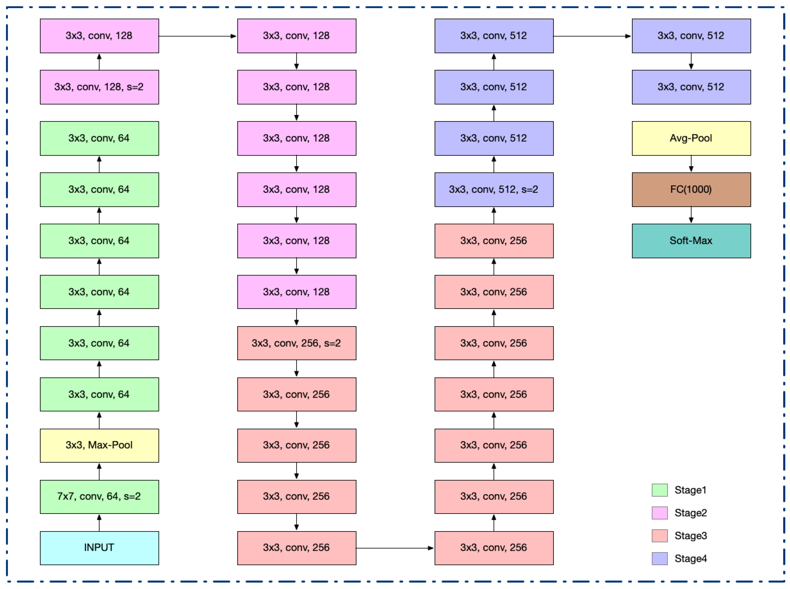
All members contain five convolution blocks (Conv1–5x, as shown in Table 1), and each one contains one or more basic convolution calculation processes: the Conv layer, the BN (Batch Normalization) layer, and the ReLU layer. The first convolution block contains only one convolution computation. The first convolution block of the 5 classic models is exactly the same as the others, with a convolution kernel of 7 × 7 and a step size of 2. They all have all-connection layers at the end. Convolution blocks 2–5 all contain multiple residual units that are the same. In many code implementations, convolution blocks 2–5 are called Stage 1, Stage 2, Stage 3, and Stage 4. To facilitate storage and calculation, each convolution block contains one downsampling operation to reduce the image size. During implementation, the maximum pool, which has a step size of 2, is adopted in Stage 1 (Conv2x). For the other 4 convolution blocks, a convolution operation with a step size of 2 is used. Taking ResNet34 as an example, we can see the basic ResNet model structure in Figure 2.
ResNet18 is a simplified version of ResNet34. The 18 in ResNet18 refers to a total of 18 layers with different weights, including convolutional layers and fully connected layers but not batch normalization or pooling layers. In addition, the difference between ResNet34 and ResNet18 lies in the different number of residual units in each stage. There are two in the four stages of ResNet18, so the total number of layers is =(2 + 2 + 2 + 2) × 2 + 1 + 1 = 18.
In ResNet50, the residuals units of ResNet18 and 34 contain two 3 × 3 convolutional layers, whereas ResNet50 itself contains three convolutional layers of 1 × 1, 3 × 3, and 1 × 1, in that order. The channels in ResNet50 double in the output part of the first residual unit at each stage, and the number of channels inside each residual unit also changes (decreasing or increasing depending on the 1 × 1 convolution layer being adjusted), which reduces the number of parameters in the deep network. Similarly, a difference between ResNet101 and ResNet152 is the number of residual units at each stage, which is shown in detail in Table 1.

2.2.2. Squeeze-and-Excitation Networks Basics

Finding the common feature representations of transformed time-domain signal images is a nontrivial task. As shown in 3.2, these images are iconic and abstract, with various levels of deformation. In contrast, classic image classification methods deal with realistic images that contain rich color, texture, and shape information [47]. After testing the basic members of the ResNet family (the testing process will be discussed in more detail in the next section), the results still needed improvement. Therefore, squeeze-and-excitation blocks (SE blocks) were introduced to enhance the presentation performance of these ResNets.
The traditional method is to transfer the weight of the network’s feature map equally to the next layer. The core idea of SENets is to establish interdependence between modeling channels. In addition, SENets do not introduce a new spatial dimension to fuse feature channels; instead, they adopt a new “feature recalibration” strategy and adaptively correct the intensity of feature responses between the channels through the network’s global loss function. In other words, the importance of each feature channel can be automatically obtained through learning, and then the useful features can be enhanced according to their importance. Features that are not useful to the current task can be suppressed. In this way, a feature channel can be adaptively calibrated.
An SENet is composed of a series of SE blocks, which can be divided into two steps: squeeze and excitation. SENets use feature recalibration to complete the attention mechanism on the channel level, also known as the SE channel attention mechanism.
Subsequently, the squeeze operation obtains the global compressed feature vector of the current feature map by performing a global average pooling on the feature map layer. It turns each two-dimensional feature channel into a real number, and the output dimension matches the input feature channel number. The excitation operation obtains the weight of each channel in the feature map through two fully connected layers and uses the weighted feature map as the input of the next layer of the network. The parameter w (shown in Figure 3) is used to generate the weight of each feature channel; w is defined to explicitly represent the correlation between the feature channels. During recalibration, the excitation output weights are multiplied element-wise by the previous features.
As can be seen above, an SE block only relies on one set of current feature maps, so it can be easily embedded into almost all current convolutional networks. The squeeze operation compresses information while at the same time reducing the overhead of the affiliated connections. One of its classic pairings is with ResNet, and this is why SENets were introduced to improve the ResNets in this paper.
The basic structure of the SE block in Figure 3 applies to any given transformation shown in Equation (2).
F t r : X U , X R W × H × C , U R W × H × C
We can construct a corresponding SE block to perform feature recalibration. Feature map U is first produced by the squeeze operation, which aggregates feature maps across the spatial dimension, W × H, to produce channel descriptors. This descriptor embeds the global distribution of the channel’s characteristic responses so that information from the global receptive field of the network can be used by its lower layers. After that, an excitation operation is performed, in which the excitation of each channel is controlled by determining a specific sampled activation for each channel through a self-gating mechanism based on channel dependence. Feature map U is then reweighted to generate the output of the SE block, which can then be input directly into subsequent layers.

2.2.3. SENet in ResNet

As mentioned above, SE blocks were introduced as a type of attention mechanism. They allow deep neural networks to focus selectively on the most important features and suppress the less important ones. This attention mechanism is particularly useful in image classification tasks, where the model needs to identify the most relevant features in an image to make accurate predictions. An SE block achieves this by using global average pooling to summarize the feature maps along the spatial dimensions into a single vector, which is then passed through two fully connected layers. The output of the second layer is a set of weights that are used to reweight the feature maps in the residual block, enabling the network to emphasize the most important features selectively and suppress the less important ones.
To incorporate an SE block into existing deep-learning models, Jie Hu proposed combining SE blocks with ResNet models, resulting in a new type of ResNet family called SE-ResNet [38], which includes various members, such as SE-ResNet50 and SE-ResNet101, which have demonstrated state-of-the-art performance on benchmark datasets such as ImageNet.
In SE-ResNets, an SE module is inserted after the activation function in each residual block. This placement ensures that the SE module can access the feature maps before they pass to the next residual block, allowing the SE block to focus selectively on the most important features at an early stage of the network. The combination of SE block and ResNet models has been shown to improve the performance of ResNet models in various image classification tasks significantly, particularly when dealing with iconic and abstract images. SE blocks allow ResNet models to focus selectively on the most important features of an image, enabling the network to learn more discriminative representations of the data. This, in turn, improves the accuracy of the model’s predictions, especially for images that are difficult to classify.
SE-ResNet models have been extensively evaluated using various benchmark datasets, such as ImageNet and CIFAR-10, and have consistently achieved state-of-the-art performance. For example, SE-ResNet152 achieved a top-1 accuracy of 82.63% on the ImageNet dataset, which is a significant improvement over the top-1 accuracy of 76.34% achieved by the basic ResNet152 model [38]. Similarly, on the CIFAR-10 dataset, SE-ResNet models achieved a higher accuracy compared with basic ResNet models: SE-ResNet152 achieved a test accuracy of 96.54% compared with the 94.54% for ResNet152 [38].

2.3. Experimental Procedure

The experiments were conducted on a desktop computer equipped with a 13th-generation i7 chip, 32 GB RAM, and an NVIDIA 3060 ti GPU. The simulation environment was implemented using the PyTorch deep-learning framework (PyTorch version 1.7.1). Python scripts were used to read the original data from CWRU, randomly select training datasets, and transform the time-domain signals into frequency-domain signals using CWT. The programs were compiled and run using Python version 3.9, PyCharm, and Terminal.
The unprocessed data obtained from CWRU served as the basis for the original signal data. The one-dimensional signal was converted into two-dimensional color images by applying the CWT method. The REB fault image data were partitioned into five distinct training datasets called Load 0, Load 1, Load 2, Load 3, and Mix Load, representing various working load conditions. A comprehensive description of this process can be found in Section 3.1.
The study aimed to determine the DL model that achieved the best performance in detecting REB faults through a comparative experiment, which was conducted in 5 (training datasets) × 10 (DL Model) sub-experiments. The DL models included ResNet18, ResNet34, ResNet50, ResNet101, and ResNet152, as well as their follow-up versions with squeezed–excitation blocks, namely, SE-ResNet18, SE-ResNet34, SE-ResNet50, SE-ResNet101, and SE-ResNet152. The additional five SE-ResNet models were incorporated because the output parameters did not meet our expectations. The use of SENet blocks was a convenient way to augment the original models without significant architectural changes.
We analyzed all the results and compared the parameters for accuracy, precision, recall and F1 score (described in detail in Section 2.4) with each other using ResNet family models, with or without SE blocks. We concluded that SE-ResNet50 is a powerful model suited to REB detection in many conditions. A detailed analysis is in Section 4.1.
We also concluded that SE-ResNet152 is another powerful model suited to REB detection in many conditions. The detailed analysis is in Section 4.

2.4. Model Performance Metrics

Model performance metrics reflect a model’s performance. Four main performance indexes were included, P (precision), R (recall), accuracy, and F1 (F1 score), as shown in the following formula:
P r e c i s i o n = T p T p   +   F p R e c a l l = T p T p   +   F N A c u r a c y = T H T p   +   F p   +   T N   +   F N F 1   =   2   ×   p r e c i s i o n   ×   r e c a l l p r e c i s i o n   +   r e c a l l
where Tp represents the number of rolling bearing faults correctly detected; Fp is the number of fault signal types incorrectly detected as another type of fault; FN represents a specific fault type that was not detected; TN represents the number of wrong detections; TM represents the number of samples correctly labeled in the top 5 probabilities of the model’s output; T M represents the number of samples correctly labeled in the maximum probability of model’s output; and the sum of Tp, FN, Fp, and TN represents the total number of samples.

3. Results of the Experiment

3.1. Signal-to-Image Results

As previously mentioned, the experimental data were collected from CWRU and are publicly available. Using these data, we tested five wavelet basis functions to learn which was the best method. To compare their effectiveness, we processed the transformed 2D images. First, we converted images to grayscale if they were in color. Then, we calculated the probability distribution of its pixel values, which is the p in Formula (9). After that, we calculated the entropy (H) using the following formula:
H = i = 1 N p i l o g 2 p i
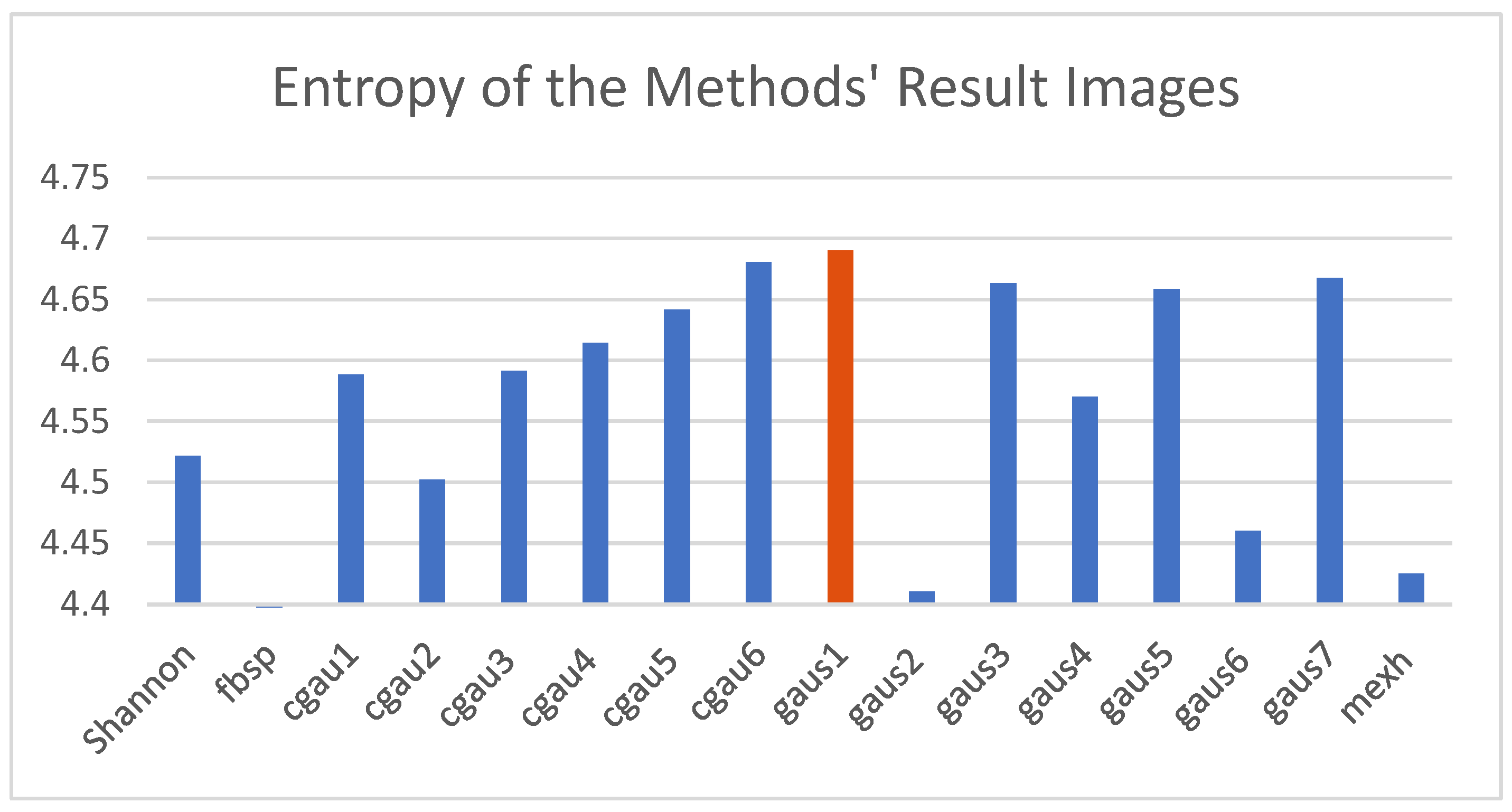
This formula calculates the entropy of the image in bits per pixel. The entropy is a measure of the average amount of information per pixel in the image. It can be used to make inferences about the image. Those with high entropy values contain more information and variation in pixel value and are more complex than images with low entropy values. The final results of the functions are as follows (Figure 4):
As shown, gaus1() had the largest entropy value, which meant that the images processed by it had better detail. Thus, it was the method we ultimately chose.
The final signal-to-image procedure is depicted in Figure 5. First, a Python script was used to read each raw data file. Next, the raw data were segmented into arrays containing 1024 sample points each, which were then converted into signal images. Eventually, the signal data were transformed into 2D images, enhancing the features extracted from the raw data.
The raw data comprised four distinct working load conditions, and each contained four REB fault conditions; thus, each load condition was separated into different training datasets. As illustrated in Table 2, five were generated: Load 0, Load 1, Load 2, Load 3, and Mix Load. Apart from the Mix Load dataset, the other four were derived directly from the raw data. The Mix Load dataset was randomly generated using samples from the other four.
In the Load 0 training dataset, there were 354 images of the inner race (IR) broken condition, 263 images of the outer race (OR) broken condition, 355 images of the ball broken condition, and 179 images of the normal working condition. In the Load 1 training dataset, there were 259 images of the IR broken condition, 264 images of the OR broken condition, 267 images of the ball broken condition, and 179 images of the normal working condition. In the Load 2 training dataset, there were 355 images of the IR broken condition, 267 images of the OR broken condition, 267 images of the ball broken condition, and 179 images of the normal working condition. In the Load 3 training dataset, there were 356 images of the IR broken condition, 268 images of the OR broken condition, 267 images of the ball broken condition, and 179 images of the normal working condition. In the Mix Load training dataset, there were 412 images of the IR broken condition, 243 images of the OR broken condition, 327 images of the ball broken condition, and 236 images of the normal working condition.
The performance of the ResNet and SE-ResNet families under each training dataset will be further discussed in the following sections.

3.2. The Results of the Fault Diagnosis

In this section, we use the signal-to-image results to verify the DL models mentioned in Section 2.3. We trained each DL model with 500 epochs using five different training datasets, as detailed in Table 2. To evaluate the performance of the DL models, we focus on four key metrics: accuracy, precision, recall, and F1 score. The remainder of this section is divided into two subsections presenting the training results for the ResNet family and the follow-up SE-ResNet family.

3.2.1. Results of ResNet Family Fault Diagnosis

As shown in Figure 6, the ResNet family DL models were evaluated using five training datasets.
For the Load 0 dataset, between the five models, ResNet50 achieved the highest accuracy at around 90%, the highest precision at over 90%, the highest recall at around 85%, and the highest F1 score at around 90%. The other four ResNet models, excluding ResNet101, achieved an almost identical performance. Specifically, their accuracy was around 80%, precision was around 70%, recall was around 70% and the F1 score was around 65%. In contrast, ResNet101 performed the worst of the ResNet models when trained on the Load 0 dataset.
For the Load 1 dataset, in contrast to the Load 0 dataset, the performance of ResNet50 and the other ResNet models was much closer. The accuracy of all models was almost the same: around 70%. Regarding precision, ResNet50 achieved the highest score at around 50%, while the other four models achieved around 40%. Similarly, ResNet50 also achieved a recall and F1 score of around 50%, and the other four models achieved a recall and F1 score of around 40%.
For the Load 2 dataset, ResNet152 achieved the highest accuracy score at around 85%, followed by ResNet34 at around 80%, ResNet18 at around 75%, ResNet50 at around 70%, and ResNet101 at around 65%. Regarding precision, ResNet50 achieved the highest precision score at around 70%, followed by ResNet152 at around 68%. ResNet34, ResNet18, and ResNet101 achieved precision scores of around 63, 58, and 50%, respectively. Similarly, the recall score for ResNet50 was the highest at around 72%, followed by ResNet152 at around 69%. ResNet34, ResNet18, and ResNet101 achieved recall scores of around 66%, 62%, and 52%, respectively. For F1 score, ResNet50 and ResNet152 achieved almost the same score at around 70%, while ResNet34 and ResNet18 achieved almost the same score at around 60%. ResNet101 achieved the lowest F1 score at around 50%.
For the Load 3 dataset, ResNet34 achieved the highest accuracy score at around 75%, followed by ResNet152 at 78%, ResNet18 at around 77%, and ResNet101 slightly higher than ResNet101 at 63%. Regarding precision, ResNet50 was significantly higher (55%) than the other four models, which achieved precision scores of around 40% or less. Similarly, the recall score for ResNet50 was the highest at around 45%, followed by ResNet34 at around 42%. The other three models achieved recall scores of under 40%.
For the Mix Load dataset ResNet34 and ResNet152 achieved almost the same accuracy scores at around 75%, followed by ResNet101 at 70%, ResNet18 at 68%, and ResNet50 at 62%. These results suggest that ResNet34 and ResNet152 were the most accurate models for the Mix Load data. Regarding precision, the performance of the models fell from ResNet152 to ResNet18, with precision scores ranging from 62 to 40%. Similarly, for recall and F1 scores, ResNet152 achieved the highest scores at around 58%, while ResNet18 achieved the lowest scores at around 40%.
The summary of this section is as follows: (1) For the Load 0 dataset, ResNet50 achieved the highest accuracy, precision, recall, and F1 scores, while the other models achieved an almost identical performance. ResNet101 performed the worst among the ResNet models. (2) For the Load 1 dataset, the performance of ResNet50 and the other ResNet models was much closer, with all models achieving almost the same accuracy scores. (3) For the Load 2 dataset, ResNet152 achieved the highest accuracy score, followed by ResNet34, ResNet18, ResNet50, and ResNet101. ResNet50 achieved the highest precision score, while ResNet50 and ResNet152 achieved the highest recall and F1 scores. (4) For the Load 3 dataset, ResNet34 achieved the highest accuracy score, while ResNet50 achieved significantly higher precision and recall scores than the other models. (5) For the Mix Load dataset, ResNet34 and ResNet152 achieved almost the same accuracy scores, while ResNet152 achieved the highest precision, recall, and F1 scores.

3.2.2. Results of the SE-ResNet Family Fault Diagnosis

As shown in Figure 7, the SE-ResNet family DL models were evaluated using five training datasets.
For the Load 0 dataset, SE-ResNet152 achieved the highest performance score of the four evaluation metrics at around 93%, followed by the other four models at around 90%. Compared with the ResNet family, the SE-ResNet family showed significant improvement in performance, particularly for SE-ResNet101, which achieved a performance score increase of over 30% compared with ResNet101.
For the Load 1 dataset, SE-ResNet50 and SE-ResNet101 achieved the highest accuracy scores at 70%; the other three models were at around 65%. Regarding precision, all models had almost the same score at around 60%, apart from SE-ResNet101. As for the recall and F1 scores, there is no obvious difference between the five models, which are all around 50%. SE-ResNet50 and SE-ResNet101 achieved the highest accuracy scores at 70%, while the other three models achieved scores of around 65%. Regarding precision, all models, except for SE-ResNet101, achieved almost the same scores of around 60%.
For the Load 2 dataset, SE-ResNet152 achieved the highest score for all four evaluation metrics, with a performance score of around 95%. SE-ResNet34, SE-ResNet50, and SE-ResNet101 achieved the same performance scores of approximately 92%, while SE-ResNet18′s performance was slightly lower than the other three models at around 90%.
For the Load 3 dataset, SE-ResNet152 achieved the highest accuracy score at 92%. SE-ResNet50 and SE-ResNet101 followed closely behind with scores of 89% and approximately 87%, respectively. For precision, recall, and F1, SE-ResNet152 achieved the highest score, with a performance of approximately 70%. The other four models scored below 70%, demonstrating that SE-ResNet152 was the most effective model for the Load 3 dataset.
For the Mix Load dataset, SE-ResNet152 achieved the highest performance score of all the models at around 96% for all four evaluation metrics. SE-ResNet152 achieved the highest score of all the models, approximately 96% across all four evaluation metrics. While the other models also performed well across all metrics, SE-ResNet50 demonstrated the weakest performance in precision, recall, and F1, with scores of approximately 70%.
Overall, SE-ResNet152 consistently achieved the highest performance scores across all datasets. The SE-ResNet family showed a significant improvement compared with the ResNet family. SE-ResNet50 and SE-ResNet101 demonstrated strong performance for certain datasets. SE-ResNet152 is the most effective model for accuracy, precision, recall, and F1 score for the Load 3 and Mix Load datasets. SE-ResNet50 demonstrated the weakest performance in precision, recall, and F1 score for the Mix Load dataset.

4. Discussion

4.1. ResNet Models

In this experiment, as mentioned in Section 2.4, we introduced four output parameters––precision, recall, accuracy, and F1 score––to describe the experimental results because accuracy alone cannot accurately describe the correctness of the training results. The larger the four kinds of data, the better this model performed. Based on the ResNet model results, the model that was the best for each corresponding situation can be seen in Figure 6.
For Load 0, ResNet50 had obvious advantages, and it was the highest of all four metrics. In the follow-up models, ResNet152, ResNet34, ResNet18, and ResNet101 were the most to least accurate, in that order. For Load 1, apart from ResNet50, the results are similar but weaker than ResNet50, especially for precision, recall, and F1 score. For Load 2, the best to worst performances were ResNet50, ResNet152, ResNet34, ResNet18, and ResNet101, in that order. The parameters of ResNet152 and ResNet34 were close, but the parameters of ResNet152 were slightly larger. For Load 3, even though the accuracy of ResNet34 was higher than ResNet50, the performance of the other three was the opposite. Thus, generally speaking, ResNet50 fit better for Load 3. For Loads 0–3, ResNet101 was always the weakest. Last but not least, for the Mixed Load, the models had better correctness as the layers increased, which meant ResNet152 was the best.
On the whole, ResNet50 was the best fit for all the conditions, as it suited most of the datasets well, or even the best. However, in the vast majority of cases, the final result was never more than 90%. We would like to improve this result, which is the reason we introduced SENet to these models.

4.2. SE-ResNet Models

As can be seen in Figure 7, the improvement the SENets bring is significant; for every 5 × 5 output, the results are better compared with the ResNet models.
For Load 0 and Load 2, four values of all five models were over 90%. In the corresponding bar chart, the results were similar to each other, and SE-ResNet152 still scored slightly better than the other models in four aspects and two conditions. For Load 1, the accuracy of SE-ResNet50 was close to that of SE-ResNet101 and a little bit higher than that of SE-ResNet18. The other two were in the next tier with SE-ResNet152 being the lowest. The recall and F1 scores shared the same trend, with SE-ResNet18, SE-ResNet50, SE-ResNet101, SE-ResNet34, and SE-ResNet152 ranging from top to bottom, in that order. Precision was 61% for SE-ResNet18, SE-ResNet50, and SE-ResNet152, followed by 60% for SE-ResNet34 and 56% for SE-ResNet101. Generally, the training-effect rankings were SE-ResNet50, SE-ResNet18, SE-ResNet34, SE-ResNet101, and SE-ResNet152, from best to worst. For Load 3, the trend was the same for all four parameters, and the order was SE-ResNet152, SE-ResNet50, SE-ResNet101, SE-ResNet34, and SE-ResNet18, from best to worst.
Even though the performance of SE-ResNet152 was not ideal for Load 1, it was the best for the other four loads. In sum, we concluded that SE-ResNet152 is the best model for all conditions.

4.3. Performance Comparison of SE-ResNet152 with Three Other DL Models

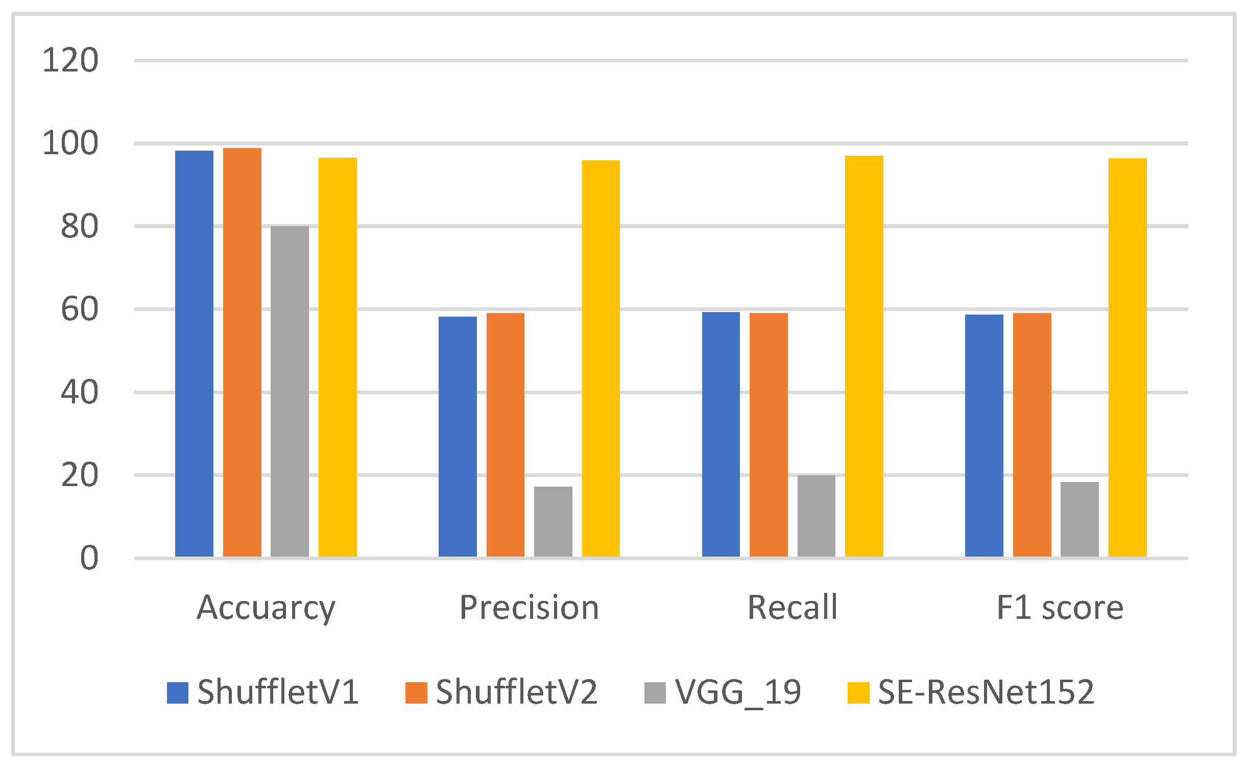
The results in Section 3.2.2 were not as ideal as we desired. Thus, we performed another test to compare the performance of SE-ResNet152 with other DL models. We conducted an experiment that involved four models: SE-ResNet152, ShuffleNetV1, ShuffleNetV2, and VGG19. The purpose was to evaluate the models’ ability to diagnose faults in rolling bearings.
The results of the experiment showed that SE-ResNet152 achieved good performance with an accuracy of 96.42%, a precision of 95.84%, a recall of 96.96%, and an F1 score of 96.31%. As per Figure 8, not only did SE-ResNet152 have accuracy in the first tier, but it also had a significant advantage in the other three parameters. The results indicated that SE-ResNet152 is a promising model for rolling bearing fault diagnosis. Put another way, the other three models, ShuffleNetV1, ShuffleNetV2, and VGG19, achieved similar accuracy scores, but their precision, recall, and F1 scores were much lower than those of SE-ResNet152.
Overall, these findings suggest that SE-ResNet152 could be an effective tool for rolling-bearing fault diagnosis, and further research could explore its potential uses in other mechanical equipment fault diagnosis tasks.

5. Conclusions

This paper proposed a fault–signal conversion method for rolling bearings based on a signal-to-image model. The signal-to-image process was achieved using continuous wavelet transform; the signal was transformed from being one-dimensional to two-dimensional, and the two-dimensional images contained more signal features. The data can be divided into five working load conditions, and based on this we trained 10 DL models to find out which ResNet model was the best for REB fault detection.
Five loads were trained using the five classic ResNet family models. Four different performance accuracy parameters were derived from the results. Through analysis and comparison, we found that the training effect of ResNet50 was the best. However, an ideal result was not achieved.
To improve the correctness of the training process, an SENet was introduced to improve the model with as few changes to the original structure as possible. To test its validity further, we compared SE-ResNet152 with the three other DL models, ShuffleNetV1, ShuffleNetV2, and VGG19, and confirmed that SE-ResNet152 is an ideal REB fault detection model.

Author Contributions

Conceptualization, G.W., X.J. and G.Y.; methodology, G.W. and Y.J.; investigation, X.J., Y.J. and C.C.; resources, G.W., X.J. and Y.J.; writing—original draft preparation, X.J. and Y.J.; writing—review and editing, G.W. and G.Y.; project administration, G.Y.; funding acquisition, G.W. All authors have read and agreed to the published version of the manuscript.

Funding

This work was supported by the Science and Technology Research Program of the Chongqing Municipal Education Commission (Grant No. KJQN202101308).

Institutional Review Board Statement

Not applicable.

Informed Consent Statement

Not applicable.

Data Availability Statement

Not applicable.

Conflicts of Interest

We declare that we do not have any commercial or associative interest that represent any conflict of interest in connection with the work submitted.

References

  1. Zhang, X.; Zhou, J. Multi-fault diagnosis for rolling element bearings based on ensemble empirical mode decomposition and optimized support vector machines. Mech. Syst. Signal Process. 2013, 41, 127–140. [Google Scholar] [CrossRef]
  2. Randall, R.B.; Antoni, J. Rolling element bearing diagnostics—A tutorial. Mech. Syst. Signal Process. 2011, 25, 485–520. [Google Scholar] [CrossRef]
  3. Dibaj, A.; Ettefagh, M.M.; Hassannejad, R.; Ehghaghi, M.B. Fine-tuned variational mode decomposition for fault diagnosis of rotary machinery. Struct. Health Monit. 2020, 19, 1453–1470. [Google Scholar] [CrossRef]
  4. Khan, S.; Yairi, T. A review on the application of deep learning in system health management. Mech. Syst. Signal Process. 2018, 107, 241–265. [Google Scholar] [CrossRef]
  5. Muruganatham, B.; Sanjith, M.; Krishnakumar, B.; Murty, S.S. Roller element bearing fault diagnosis using singular spectrum analysis. Mech. Syst. Signal Process. 2013, 35, 150–166. [Google Scholar] [CrossRef]
  6. McFadden, P.; Smith, J. Vibration monitoring of rolling element bearings by the high-frequency resonance technique—A review. Tribol. Int. 1984, 17, 3–10. [Google Scholar] [CrossRef]
  7. Lu, C.; Wang, Z.; Zhou, B. Intelligent fault diagnosis of rolling bearing using hierarchical convolutional network based health state classification. Adv. Eng. Inform. 2017, 32, 139–151. [Google Scholar] [CrossRef]
  8. Singh, M.; Shaik, A.G. Faulty bearing detection, classification and location in a three-phase induction motor based on Stockwell transform and support vector machine. Measurement 2019, 131, 524–533. [Google Scholar] [CrossRef]
  9. Gharesi, N.; Arefi, M.M.; Ebrahimi, Z.; Razavi-Far, R.; Saif, M.; Zarei, J. Analyzing the vibration signals for bearing defects diagnosis using the combination of SGWT feature extraction and SVM. IFAC-Pap. 2018, 51, 221–227. [Google Scholar] [CrossRef]
  10. Caesarendra, W.; Pratama, M.; Kosasih, B.; Tjahjowidodo, T.; Glowacz, A. Parsimonious network based on a fuzzy inference system (PANFIS) for time series feature prediction of low speed slew bearing prognosis. Appl. Sci. 2018, 8, 2656. [Google Scholar] [CrossRef]
  11. Glowacz, A. Fault detection of electric impact drills and coffee grinders using acoustic signals. Sensors 2019, 19, 269. [Google Scholar] [CrossRef] [PubMed]
  12. Xu, Y.; Zhang, K.; Ma, C.; Cui, L.; Tian, W. Adaptive Kurtogram and its applications in rolling bearing fault diagnosis. Mech. Syst. Signal Process. 2019, 130, 87–107. [Google Scholar] [CrossRef]
  13. Liu, Z.; Yang, S.; Liu, Y.; Lin, J.; Gu, X. Adaptive correlated Kurtogram and its applications in wheelset-bearing system fault diagnosis. Mech. Syst. Signal Process. 2021, 154, 107511. [Google Scholar] [CrossRef]
  14. Zhang, K.; Xu, Y.; Liao, Z.; Song, L.; Chen, P. A novel Fast Entrogram and its applications in rolling bearing fault diagnosis. Mech. Syst. Signal Process. 2021, 154, 107582. [Google Scholar] [CrossRef]
  15. Cheng, J.; Yang, Y.; Li, X.; Cheng, J. Adaptive periodic mode decomposition and its application in rolling bearing fault diagnosis. Mech. Syst. Signal Process. 2021, 161, 107943. [Google Scholar] [CrossRef]
  16. Yosinski, J.; Clune, J.; Bengio, Y.; Lipson, H. How transferable are features in deep neural networks? Adv. Neural Inf. Process. Syst. 2014, 27, 3320–3328. [Google Scholar]
  17. Krizhevsky, A.; Sutskever, I.; Hinton, G.E. Imagenet classification with deep convolutional neural networks. Commun. ACM 2017, 60, 84–90. [Google Scholar] [CrossRef]
  18. Chen, H.; Liu, Z.; Alippi, C.; Huang, B.; Liu, D. Explainable intelligent fault diagnosis for nonlinear dynamic systems: From 522 unsupervised to supervised learning. IEEE Trans. Neural Netw. Learn. Syst. 2022. [Google Scholar] [CrossRef]
  19. Fu, W.; Tan, J.; Xu, Y.; Wang, K.; Chen, T. Fault diagnosis for rolling bearings based on fine-sorted dispersion entropy and SVM optimized with mutation SCA-PSO. Entropy 2019, 21, 404. [Google Scholar] [CrossRef]
  20. Wei, Y.; Li, Y.; Xu, M.; Huang, W. A review of early fault diagnosis approaches and their applications in rotating machinery. Entropy 2019, 21, 409. [Google Scholar] [CrossRef]
  21. Suykens, J.A.; Vandewalle, J. Least squares support vector machine classifiers. Neural Process. Lett. 1999, 9, 293–300. [Google Scholar] [CrossRef]
  22. Schmidhuber, J. Deep learning in neural networks: An overview. Neural Netw. 2015, 61, 85–117. [Google Scholar] [CrossRef] [PubMed]
  23. Chen, Z.; Li, C.; Sanchez, R.V. Gearbox fault identification and classification with convolutional neural networks. Shock. Vib. 2015, 2015, 390134. [Google Scholar] [CrossRef]
  24. Zhao, J.; Yang, S.; Li, Q.; Liu, Y.; Gu, X.; Liu, W. A new bearing fault diagnosis method based on signal-to-image mapping and convolutional neural network. Measurement 2021, 176, 109088. [Google Scholar] [CrossRef]
  25. Zhang, W.; Li, C.; Peng, G.; Chen, Y.; Zhang, Z. A deep convolutional neural network with new training methods for bearing fault diagnosis under noisy environment and different working load. Mech. Syst. Signal Process. 2018, 100, 439–453. [Google Scholar] [CrossRef]
  26. Janssens, O.; Slavkovikj, V.; Vervisch, B.; Stockman, K.; Loccufier, M.; Verstockt, S.; Van de Walle, R.; Van Hoecke, S. Convolutional neural network based fault detection for rotating machinery. J. Sound Vib. 2016, 377, 331–345. [Google Scholar] [CrossRef]
  27. Springenberg, J.T. Unsupervised and semi-supervised learning with categorical generative adversarial networks. arXiv 2015, arXiv:1511.06390. [Google Scholar]
  28. Gao, Y.; Liu, X.; Huang, H.; Xiang, J. A hybrid of FEM simulations and generative adversarial networks to classify faults in rotor-bearing systems. ISA Trans. 2021, 108, 356–366. [Google Scholar] [CrossRef]
  29. Liu, H.; Zhou, J.; Xu, Y.; Zheng, Y.; Peng, X.; Jiang, W. Unsupervised fault diagnosis of rolling bearings using a deep neural network based on generative adversarial networks. Neurocomputing 2018, 315, 412–424. [Google Scholar] [CrossRef]
  30. Wang, R.; Jiang, H.; Li, X.; Liu, S. A reinforcement neural architecture search method for rolling bearing fault diagnosis. Measurement 2020, 154, 107417. [Google Scholar] [CrossRef]
  31. Liu, H.; Zhou, J.; Zheng, Y.; Jiang, W.; Zhang, Y. Fault diagnosis of rolling bearings with recurrent neural network-based autoencoders. ISA Trans. 2018, 77, 167–178. [Google Scholar] [CrossRef]
  32. Guo, L.; Li, N.; Jia, F.; Lei, Y.; Lin, J. A recurrent neural network based health indicator for remaining useful life prediction of bearings. Neurocomputing 2017, 240, 98–109. [Google Scholar] [CrossRef]
  33. Tamilselvan, P.; Wang, P. Failure diagnosis using deep belief learning based health state classification. Reliab. Eng. Syst. Saf. 2013, 115, 124–135. [Google Scholar] [CrossRef]
  34. Shao, H.; Jiang, H.; Zhang, X.; Niu, M. Rolling bearing fault diagnosis using an optimization deep belief network. Meas. Sci. Technol. 2015, 26, 115002. [Google Scholar] [CrossRef]
  35. Shao, H.; Jiang, H.; Zhang, H.; Duan, W.; Liang, T.; Wu, S. Rolling bearing fault feature learning using improved convolutional deep belief network with compressed sensing. Mech. Syst. Signal Process. 2018, 100, 743–765. [Google Scholar] [CrossRef]
  36. Lu, C.; Wang, Z.Y.; Qin, W.L.; Ma, J. Fault diagnosis of rotary machinery components using a stacked denoising autoencoder-based health state identification. Signal Process. 2017, 130, 377–388. [Google Scholar] [CrossRef]
  37. He, K.; Zhang, X.; Ren, S.; Sun, J. Deep residual learning for image recognition. In Proceedings of the IEEE Conference on Computer Vision and Pattern Recognition, Las Vegas, NV, USA, 27–30 June 2016; pp. 770–778. [Google Scholar]
  38. Hu, J.; Shen, L.; Sun, G. Squeeze-and-excitation networks. In Proceedings of the IEEE Conference on Computer Vision and Pattern Recognition, Salt Lake City, UT, USA, 18–23 June 2018; pp. 7132–7141. [Google Scholar]
  39. Huang, G.; Liu, Z.; Van Der Maaten, L.; Weinberger, K.Q. Densely connected convolutional networks. In Proceedings of the IEEE Conference on Computer Vision and Pattern Recognition, Honolulu, HI, USA, 21–26 July 2017; pp. 4700–4708. [Google Scholar]
  40. Xie, S.; Girshick, R.; Dollár, P.; Tu, Z.; He, K. Aggregated residual transformations for deep neural networks. In Proceedings of the IEEE Conference on Computer Vision and Pattern Recognition, Honolulu, HI, USA, 21–26 July 2017; pp. 1492–1500. [Google Scholar]
  41. Parmar, A.; Gulia, S.; Bajaj, S.; Gambhir, V.; Sharma, R.; Reddy, M. Signal processing of Raman signatures and realtime identification of hazardous molecules using continuous wavelet transformation (CWT). In Proceedings of the 2015 International Conference on Signal Processing and Communication Engineering Systems, Guntur, India, 2–3 January 2015; pp. 323–325. [Google Scholar]
  42. Nigrin, A. Neural Networks for Pattern Recognition; MIT Press: Cambridge, MA, USA, 1993. [Google Scholar]
  43. Simonyan, K.; Zisserman, A. Very deep convolutional networks for large-scale image recognition. arXiv 2014, arXiv:1409.1556 527. [Google Scholar]
  44. Bengio, Y.; Simard, P.; Frasconi, P. Learning long-term dependencies with gradient descent is difficult. IEEE Trans. Neural Netw. 1994, 5, 157–166. [Google Scholar] [CrossRef]
  45. Goodfellow, I.; Warde-Farley, D.; Mirza, M.; Courville, A.; Bengio, Y. Maxout networks. In Proceedings of the International Conference on Machine Learning, Atlanta, GA, USA, 16–21 June 2013; pp. 1319–1327. [Google Scholar]
  46. Le, Y.; Bottou, L.; Orr, G. Efficient BackProp. In Neural Networks: Tricks of the Trade; Springer: Berlin/Heidelberg, Germany, 1998. [Google Scholar]
  47. Jajodia, T.; Garg, P. Image classification–cat and dog images. Image 2019, 6, 570–572. [Google Scholar]
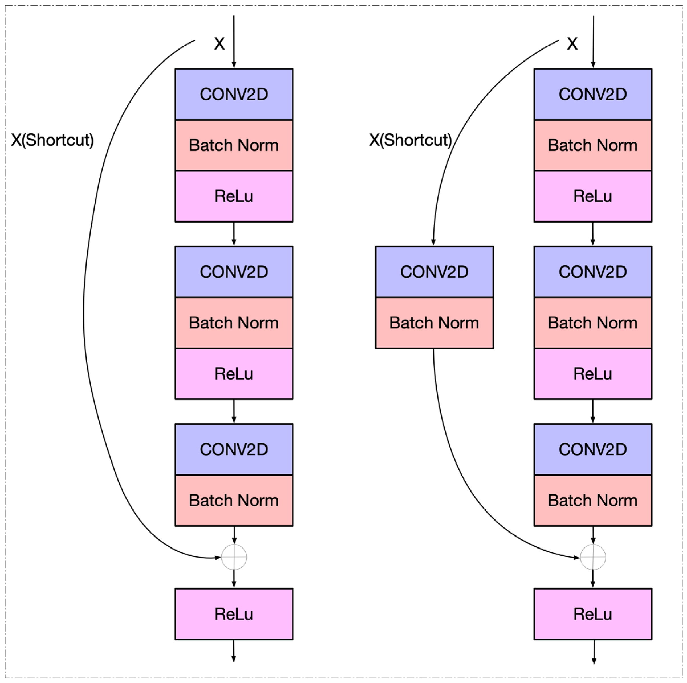
Figure 1. Two main ResNet blocks.
Processes 11 01527 g001
Figure 2. The structure of ResNet34.
Processes 11 01527 g002
Figure 3. A squeeze-and-excitation block.
Processes 11 01527 g003
Figure 4. Comparison of CWT method entropy values.
Processes 11 01527 g004
Figure 5. The signal-to-image process.
Processes 11 01527 g005
Figure 6. Detecting fault data using ResNets.
Processes 11 01527 g006
Figure 7. Detecting fault data using SE-ResNets.
Processes 11 01527 g007
Figure 8. The detection results of the four models.
Processes 11 01527 g008
Table 1. ResNet family.
Layer NameOutput Size18-Layer34-Layer50-Layer101-Layer152-Layer
conv1112 × 1127 × 7, 64, stride 2
conv2x56 × 563 × 3 max pool, stride 2
3 × 3 ,   64 3 × 3 ,   64 × 2 3 × 3 ,   64 3 × 3 ,   64 × 3 1 × 1 ,   64 3 × 3 ,   64 1 × 1 ,   256 × 3 1 × 1 ,   64 3 × 3 ,   64 1 × 1 ,   256 × 3 1 × 1 ,   64 3 × 3 ,   64 1 × 1 ,   256 × 3
conv3x28 × 28 3 × 3 ,   128 3 × 3 ,   128 × 2 3 × 3 ,   128 3 × 3 ,   128 × 4 1 × 1 ,   128 3 × 3 ,   128 1 × 1 ,   512 × 4 1 × 1 ,   128 3 × 3 ,   128 1 × 1 ,   512 × 4 1 × 1 ,   128 3 × 3 ,   128 1 × 1 ,   512 × 8
conv4x14 × 14 3 × 3 ,   256 3 × 3 ,   256 × 2 3 × 3 ,   256 3 × 3 ,   256 × 6 1 × 1 ,   256 3 × 3 ,   256 1 × 1 ,   1024 × 6 1 × 1 ,   256 3 × 3 ,   256 1 × 1 ,   1024 × 23 1 × 1 ,   256 3 × 3 ,   256 1 × 1 ,   1024 × 36
conv5x7 × 7 3 × 3 ,   512 3 × 3 ,   512 × 2 3 × 3 ,   512 3 × 3 ,   512 × 3 1 × 1 ,   512 3 × 3 ,   512 1 × 1 ,   2048 × 3 1 × 1 ,   512 3 × 3 ,   512 1 × 1 ,   2048 × 3 1 × 1 ,   512 3 × 3 ,   512 1 × 1 ,   2048 × 3
1 × 1Average pool, 1000-d fc, softmax
FLOPs1.8 × 1093.6 × 1093.8 × 1097.6 × 10911.3 × 109
Table 2. Training datasets.
Load 0Load 1Load 2Load 3Mix
IR354259355356412
OR263264267268243
Ball355267267267327
Normal179179179179236
Disclaimer/Publisher’s Note: The statements, opinions and data contained in all publications are solely those of the individual author(s) and contributor(s) and not of MDPI and/or the editor(s). MDPI and/or the editor(s) disclaim responsibility for any injury to people or property resulting from any ideas, methods, instructions or products referred to in the content.