1. Introduction
This paper presents an improved version of the MDDB-GC clustering data stream algorithm. Specifically, it begins with an overview of recent developments in data stream clustering algorithms, highlighting their respective advantages and disadvantages as well as common challenges. To address these issues, an enhanced variant of the MDDSDB-GC algorithm is proposed, followed by a detailed description of its steps. The accuracy and practicality of the proposed algorithm are then evaluated through rigorous experiments.
1.1. Concept and Characteristics of Data Streams
People are living in an age of data explosion with the arrival of high-tech communication and information. In many applications, data with randomness, high speed, continuous arrival, and infinity are called data streams. The data stream can be understood from both narrow and broad perspectives.
From the narrow perspective, data stream is when a large quantity of data become changeful and grow infinitely. For example, the data packets processed by routers and sensor network data are typical representatives of this data stream data. In a broad sense, data stream refers to the large-scale data set that can only perform linear scanning operations, such as customer click stream, collection of web pages, multimedia data, financial transactions, scientific observation data, etc.
The data stream has characteristics that differ from static data, which can be summarized as follows:
Data streams are too large to be stored in a memory or hard disk way, which can only save some data sets or approximate statistical information. Similarly, the analysis of data flow can only be scanned once, and the data cannot be scanned as many times as the traditional data clustering algorithm.
- (1)
High dimension. The data stream may have a high dimension, and high-dimensional data processing is more complex than low-dimensional data.
- (2)
Velocity. Since the data stream is fast to arrive, it is unrealistic and inaccurate to obtain the results by accurately analyzing a single data element, but is more accurate by analyzing the summary information of some data elements or data sets.
- (3)
Temporality. The data streams arrive based on chronological order, and the historical data will be gradually deleted with the decay of time. Therefore, the data elements in the data stream cannot be accessed randomly, but can be read once or several times according to the time order.
- (4)
Persistence. A continuous stream of data will grow in an indefinite way. The result of the data stream processing will not be the final one due to the endless characteristics, thus, the data stream processing technology shall be a continuous process.
1.2. Requirements for Data Stream Clustering
In the advent of big data, in many application scenarios, such as in the industrial field and transportation field, the demand for cluster analysis of data streams is huge. However, due to the characteristics of the data stream, the traditional algorithm is not enough to meet the high demand of the clustering algorithm. The traditional clustering algorithm is based on the database operation mode where the database can store all data and support complex query operations. However, in the data stream environment, these methods are not feasible. Therefore, a data stream clustering algorithm must have the following characteristics at the same time [
1]:
Firstly, limited storage capacity. The data stream clustering algorithm cannot store all the data objects that need to be processed, and it shall ensure a reasonable capacity by selectively abandoning the data.
Secondly, linear and one-time scanning. The data stream clustering algorithm should only perform linear and one-time scanning, and at least achieve incremental processing of linear scanning.
Thirdly, good real-time performance for the processing and analysis of data records. The updating speed of massive data in the data stream is very fast, and the requirement for the completion speed of calculation and analysis is very high.
Fourthly, some operations which can be used in database applications, in a data stream environment are failed to be used (such as Blocking and Sort).
In addition, the data stream clustering algorithm should also have some other characteristics:
Insensitivity to the input order of data. Data arrival in the data stream is an uncontrollable factor, and the data stream clustering algorithm can only process passively according to the order of arrival of data.
- (1)
Adaptability to any shape. The shape and number of data classes in data streams often change over time. Therefore, the data stream clustering method should have good adaptability to the clustering of arbitrary shapes.
- (2)
Tracking ability of data clustering. The application requirements of some data stream environments are not to query the distribution and change of “past” data, but the data model is updated in real time and used in subsequent processing.
1.3. The Introduction of the Existing Data Stream Clustering Algorithms
The algorithm of incremental feature applies to data stream clustering analysis, and the representation of clustering should be concise and accurate. New data should be processed quickly and effectively and be robust regarding noise and abnormal data. Since a data stream can be regarded as an infinite process that changes over time, the implicit clustering may change over time, so the previously generated clustering is no longer applicable to the current situation, resulting in a decrease in clustering quality. Following is a quick introduction to a few potential data stream clustering methods.
Several scholars have proposed various algorithms to improve the clustering quality of data streams. Jia Dongli and other experts [
2] have suggested dynamically adjusting window size and incorporating micro-cluster structures for better clustering results. Wan Xingui [
3] has proposed a distributed data stream clustering method that combines online and offline parts, while Mei Yingyinyin and Liang Yuefang [
4] have proposed an algorithm that integrates data stream clustering into intrusion detection with improved clustering based on attenuation sliding window density. In addition, Mansheng Xiao and Yongxiang Hu [
5] have introduced the IU-IFCM algorithm that uses an improved fuzzy C-means technique for interval data clustering, and Niu Liyuan [
6] has proposed the DBS-Stream algorithm, which is a distributed real-time density clustering algorithm for data streams based on Clu-Stream and DBSCAN. Moreover, Yingfeng Tang and other scholars [
7] have introduced a clustering method for distributed data streams in intelligent transportation systems that utilizes grid blocks to enable incremental clustering and merging, and Wu Dechao [
8] has optimized the traditional K-means clustering algorithm using the Canopy algorithm and the “maximum and minimum principle” in Hadoop to improve efficiency and accuracy. Experts Sun and Chen [
9] proposed a weight attenuation WDSMC-based fuzzy micro-cluster clustering technique for data streams to address time and capacity limitations. This technique utilizes the improved fuzzy C-means algorithm with weights, micro-cluster structures, and weight time attenuation to enhance clustering quality. Finally, Hadali [
10] has proposed a novel algorithm for clustering big data with varying densities using the MapReduce framework in Hadoop, which leverages local density to address clustering challenges and exhibits superior scalability.
In addition, Li Mingyang [
11] proposed a new two-stage clustering method based on the improved DBSCAN and DP algorithm (TSCM) in 2019. The improved DBSCAN uses a well-known internal clustering validation index without labels, called Silhouette, using bat optimization to regulate the parameter determination procedure using the fitness function. The cluster centers in the decision graph are automatically selected according to the initial cluster. The final clustering is obtained by DP and has a determined cluster center. Compared with DP and DBSCAN, TSCM can effectively overcome the manual intervention of cluster center selection in DP and parameters setting in DBSCAN. The clustering performance is significantly improved. Nooshin Hanafi [
12] lately proposed an improved DBSCAN. Compared to the original DBSCAN algorithm, large dataset processing is better suited to it. The program then suggested a technique to precisely compute each sample density based on a condensed set of data, known as the operational set, and it would update on a regular basis. This algorithm can detect clusters of various forms and does not require prior clusters.
1.4. Summary of Existing Data Stream Clustering Algorithms
In conclusion, the data stream clustering algorithms that are now in use are the data stream clustering algorithm based on grid and density and the data stream clustering method based on K-means and K-center points.
On the one hand, the data stream clustering algorithm based on the clustering idea of K-means and K-center points is formed by improving them to adjust for the data stream’s properties (such as one-time scanning). Although the design of these algorithms adapts to the characteristics of the data stream and achieves good results, the partition-based method determines two common shortcomings. First, it is necessary to determine the number of clusters k through prior knowledge, which is usually difficult to achieve. Second, their clustering results also tend to be spherical, which is difficult to be competent in the face of complex arbitrary clustering.
On the other hand, the grid- and density-based data stream clustering method converts the data in the data stream or the summary data reflecting the data stream into a “static” data set at a specific moment, and then carries out the subsequent clustering calculation based on this “static” data set. The obtained clustering results are static results for this data set. This method, which employs a data-stream-oriented static clustering algorithm, was created primarily to satisfy the demands of the “query” on the distribution of “previous” data and distribution changes. However, its shortcomings are that it does not pay attention to the automatic analysis of clustering changes, and the analysis results are applied to the subsequent processing. When dealing with data stream applications with high real-time requirements, it often cannot meet the requirements.
Given the defects of the above two types of data stream clustering algorithms, the goal of this study is to try to innovate a data stream clustering algorithm with better performance. This algorithm can realize dynamic data stream clustering analysis without prior knowledge and can find arbitrary shape clustering.
2. Original Algorithm MDDB-GC
In this work, we aim to improve the multi-Density DBSCAN clustering algorithm based on grid and contribution, also known as the MDDB-GC algorithm. To provide context, we first provide a brief introduction to the conventional DBSCAN, multi-density DBSCAN, and MDDB-GC algorithms.
According to the previous research results, we found that the multi-density DBSCAN clustering algorithm based on grid and contribution proposed by Lin-meng Zhang [
13], namely, the GCMDDBSCAN (In this article, we adopt MDDB-GC to refer to the proposed algorithm.) algorithm, has relatively good characteristics, but there are also some defects, which are suitable for optimization and improvement as the original algorithm of the target algorithm. The advantages of the MDDB-GC algorithm are: prior knowledge is not necessary, arbitrary shape clustering can be found, anti-interference of noise, multi-density clustering can be effectively distinguished, and large-scale data sets can be processed. The defect of the MDDB-GC algorithm is that the three important parts of the algorithm, i.e., the calculation methods of contribution, grid density, and migration factor, cannot meet the basic requirements of the data stream analysis algorithm. Therefore, it is necessary to improve the algorithm to realize the data stream clustering analysis.
Since the MDDB-GC algorithm is developed from the improvement of conventional DBSCAN and multi-density DBSCAN algorithms (MD-DBSCAN), the conventional DBSCAN, multi-density DBSCAN, and MDDB-GC algorithms are briefly introduced in the following.
2.1. Introduction to Conventional DBSCAN Algorithm
DBSCAN is a density-based clustering algorithm. Clusters with any shapes may be identified in spatial databases with “noise”, which defines clusters as the maximum set of points related to density. The method splits regions with sufficiently high density into clusters, and clusters with arbitrary shapes can be found there.
The idea of the algorithm based on DBSCAN is to start with any point p in dataset D to find all the points that can be reached from p density concerning
ε and MinPts in D. If
P is a core point, then all points in its neighborhood area belong to the same cluster of
P.
P is temporarily marked as noise if it is not the core point, that is, if no object can be reached from the density of
P, which will serve as inspection objects of the following round (referred to as seed points), and extend their cluster by continuously finding points that can be reached from the seed point density until a complete cluster is found. The program then repeats the procedure described above for the next item in D. When all seed points are examined, a cluster is expanded. At this stage, the algorithm will expand another cluster if there are any unprocessed points in D, otherwise, unprocessed points in D are considered noise. Then, in 2012, K. Dominik and K. Jens [
14] suggested a modified version of the most widely used and referenced clustering method, known as DBSCAN, to cope with the non-equidistant sampling density and clutter of radar data while retaining all of its previous benefits. In addition, it is resistant to clutter and performs an optimum separation of items using a variety of sampling resolutions.
Although DBSCAN can find clusters of different shapes and sizes, it has trouble finding clusters of different densities because of its parameter Eps. Ahmed Fahim [
15] introduces a novel technique for finding clusters of various densities that begins with any item and computes the local density of each object as the sum of distances to its k1-nearest neighbors. This technique is known as cluster initiator. Then, considering any object is reachable from a cluster initiator and has a local density similar to the local density of the cluster initiator is assigned the same cluster. The method needs a threshold for SR (Similarity Ratio). The proposed method solves the problem of different densities, shapes, and sizes, giving a superior ability of detection for different densities. Hou SiZu [
16] proposed an improved DBSCAN as well, in order to adapt to varied densities. To create a density threshold that is appropriate for the data density, first preprocess the data and determine the density surrounding each data item. Additionally, before the clustering process was complete, a density threshold was employed to increase the effectiveness of the proposed technique in grouping data with various densities and arbitrary shapes. Chen Jungan [
17] proposed a clustering algorithm based on artificial immune system, which uses a deviation factor model to describe the data distribution. It calculates the deviation factor based on the maximum and average distance, overcoming the difficulty of finding non-spherical shapes or varied size and density.
2.2. Multi-Density DBSCAN Algorithm
The advantages of the conventional DBSCAN algorithm are as follows: Firstly, it can effectively shield the interference of noise data. Secondly, it can cluster arbitrary shape spatial distribution data sets. Because of these outstanding advantages, the DBSCAN algorithm has high practical application value. However, the conventional DBSCAN algorithm has two shortcomings. First, the clustering result is highly dependent on the parameter setting and is especially sensitive to the parameter Eps. The accurate Eps value needs to be set based on prior knowledge to obtain better clustering results. Second, when the spatial distribution of data sets presents multiple different density regions and the density difference between each other is large, the conventional DBSCAN will not be able to cluster correctly because of the global unique Eps value.
Given the defects of the conventional DBSCAN algorithm, G. Esfandani and H. Abolhassani [
18] in 2010 proposed MSDBSCAN, using a new definition for core point and dense area. In multi-variant density data sets, the MSDBSCAN can locate clusters and offers scale independence. After that, the multi-density DBSCAN algorithm proposed by Wesam Ashour and Saad Sunoalla [
19] in 2011 achieved better clustering results because it effectively solved the global unique Eps value limitation and the parameter setting dependence problem to a certain extent.
In Wesam Ashour’s research, the average distance between data points and the average distance inside a cluster, which are described as follows, replace the parameter Eps in this multi-density DBSCAN method.
Definition 1. (Data point P’s average distance value, DSTp) The average spatial distance between data point P and its closest k data points, or the average distance value DSTp of data point P, for a given constant k (k is a natural integer).
Definition 2. (AVGDST, average distance within a cluster) For a given constant k (k is a natural number), the average value of DSTp of all data points within a cluster, i.e., average distance AVGDST within this cluster.
As can be seen, the real density status at data point P and a particular cluster are better described by the average distance value of the data point P and the average distance value inside the cluster. This algorithm divides mainly based on the two average distance values and distinguishes the classification of different densities, thus realizing the clustering of the whole data set.
2.3. Introduction of MDDB-GC Algorithm
There are still some defects in the multi-density DBSCAN algorithm. In the clustering process, like the conventional DBSCAN algorithm, it is still necessary to scan the entire data set to calculate and find the set of k nearest data points of a data point. Therefore, there are a large number of invalid calculations. The computing efficiency is low, and it is incapable of handling massive data sets. Therefore, some scholars [
20] introduced the idea of a grid clustering algorithm and combined it with the concept of “contribution” to propose an improved algorithm MDDB-GC.
MDDB-GC algorithm is an improved algorithm based on a multi-density DBSCAN algorithm by introducing gridding technology, contribution, and migration factor. This improvement is mainly reflected in the following three aspects: (1) The use of grid-boxing techniques and tree index structures enhances the ability to process large-scale datasets. After introducing grid technology, the main analysis object of the MDDB-GC algorithm is transformed from a large number of data points to a certain number of grids, so it is more efficient to deal with large-scale data sets. At the same time, when calculating the set of adjacent data points, it does not need to scan the entire data set, and only needs to use the tree index structure to search the adjacent grid; (2) The formula for grid density may be generated based on the idea of “contribution”, and the geographical distribution of the data points in the grid can be completely taken into account. This allows the clustering outcomes to be maximized without adding more grids; (3) Migration factors can optimize boundary data points. The fixed grid division method is simple and easy, but boundary data points are often misjudged as noise points and then ignored, and for better clustering, the migration factor is concerned with border data points.
3. Proposed Algorithm: MDDB-GC Algorithm
In this section of the study, a systematic presentation of the MDDB-GC research content will be provided, which encompasses the genesis of the research idea and a comprehensive exposition of the grid’s contributions and other significant factors.
3.1. Main Idea
This study hopes to create a data stream clustering algorithm with better performance that can achieve dynamic, without prior knowledge, and can find arbitrary shape clustering. The MDDB-GC algorithm proposed by scholars has the advantages of no prior knowledge, discovering arbitrary shape clustering, resisting noise interference, effectively distinguishing multi-density clustering, and processing large-scale data sets. However, the algorithm has three important parts, namely, the calculation method of contribution, grid density, and migration factor, which cannot meet the basic requirements of the data stream analysis algorithm. Therefore, the MDDB-GC algorithm is selected as the original algorithm, and the calculation methods of contribution, grid density, and migration factor are effectively improved. At the same time, the other parts are adjusted to innovate the new algorithm. The new algorithm is an improved MDDB-GC algorithm for the data stream, abbreviated as the MDDSDB-GC algorithm (Multi-Density DBSCAN clustering algorithm based on grid and contribution for Data Stream).
3.2. Grid Division
The number of separated grids affects both the computational cost of the grid-based clustering technique and the final clustering result. Moreover, computational complexity and clustering effect are usually opposite. The finer the partition granularity is, the greater the number of grids, and the better the clustering effect, but the computational complexity greatly increases. On the contrary, the rougher the partition granularity is, the less the number of grids, and the computational complexity is greatly reduced, but the clustering effect becomes worse. In this algorithm, a relatively simple fixed grid division method can be used to complete the grid division.
Definition 3. (Grid element) In a given d-dimensional data space S, each dimension is divided into L equal-length and disjoint left-closed and right-open regions, so that the data space S is divided into Ld equal-size and disjoint hyperrectangular elements. Each such super-rectangular element is a grid element corresponding to the division (hereinafter referred to as grid).
To achieve grid division, it is necessary to standardize the data points in
d-dimensional data space
S, such as changing the value line of each dimension’s data points into the range (0,1]. The range space is then evenly split into
L segments on each dimension, and the value of
L may be found by using the following equation.
In Equation (1), is the total number of data points, int(x) is the integer of x, is the adjustment coefficient, and the value range is usually (0, 1]. The larger the value of is, the finer the partition granularity. The specific value of needs to be determined by considering the computational complexity and clustering effect.
In this algorithm, due to the role of contribution and migration factor, the clustering effect can be improved without increasing the computational complexity to some extent, so the selection of value can be appropriately reduced to reduce the operation time. A large number of experiments show that for data stream clustering analysis, can be valued [0.2, 0.6].
3.3. Tree Index Structure: SP-Tree
SP-Tree is called Spatial Partition Tree. When dealing with multi-dimensional or even high-dimensional large-scale data sets, effective tree index structure is a crucial auxiliary factor. This algorithm implements data and region queries by SP-Tree to improve calculation efficiency. In this algorithm, three SP-Trees are created under spatial grid division, corresponding to the indexed non-empty grid, dense grid, and sparse grid.
Definition 4. (SP-Tree) d-dimensional dataset S generates SP-Tree structure under partition P as follows:
- (1)
SP-Tree has a (d + 1) layer, where d is the latitude of the dataset.
- (2)
There is only one path from the root node to the leaf node, and this path corresponds to a grid that needs an index.
- (3)
The -layer node is the -dimensional interval number of the indexed grid and refers to the (+ 1) layer node in addition to the (d + 1) layer.
The leaf nodes of the (d + 1) layer correspond to the grid information of the index. In this algorithm, the leaf node contains information such as the location of data points in the grid, the migration factor of data points, and the cumulative contribution.
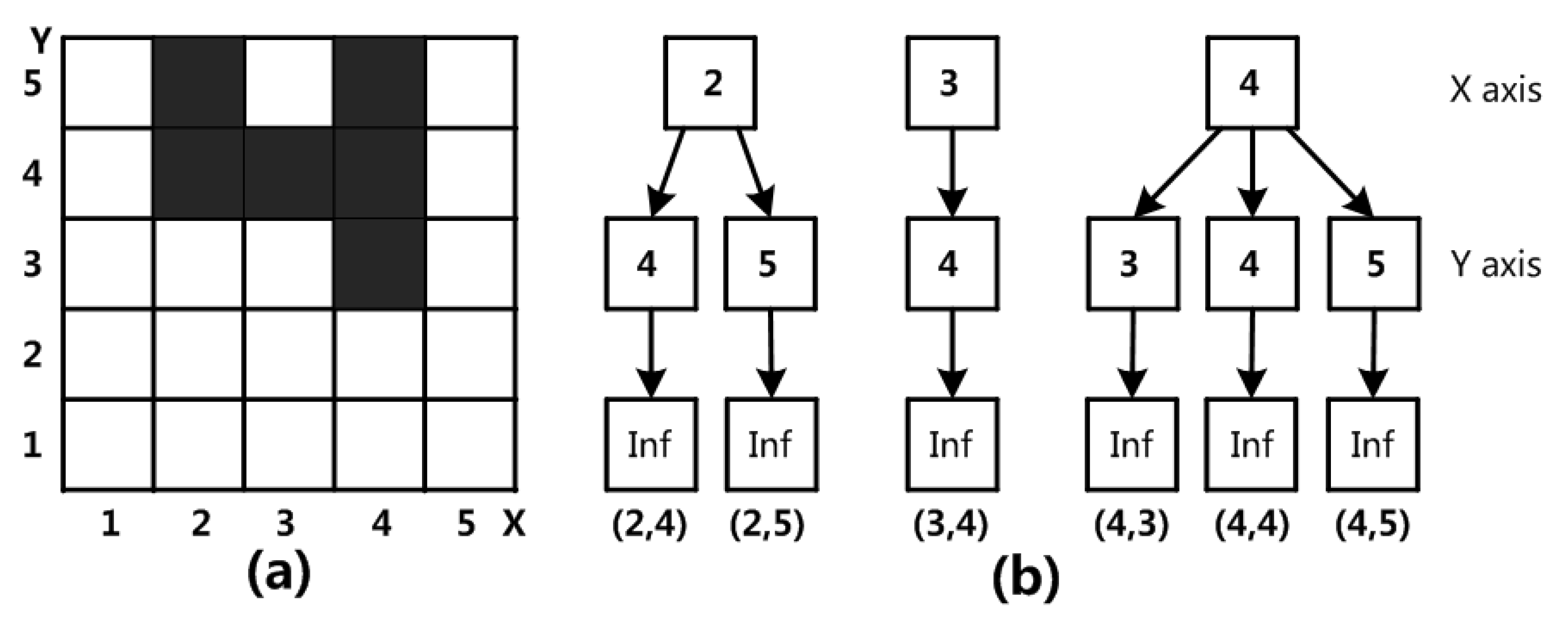
Figure 1a shows the grid structure of two-dimensional data space under a certain division. Each dimension is divided into five interval segments. The gray-black grid is the grid that needs an index.
Figure 1b shows the SP-Tree structure that requires an index grid. The SP-Tree is divided into three layers. The index grid’s X- and Y-dimensional interval numbers are located in the top two levels. The leaf node layer is the bottom layer. The data of the index grid are stored in each leaf node.
In this algorithm, the grid data information, in addition to the original information, extended to the data stream clustering analysis, needs to add two important pieces of information. Among them, the original information pertains to the total number of data points in the grid, their locations, their migration factors within each dimension, their k closest neighbors and their separation, as well as the grid’s overall contribution. Two new important pieces of information are the new Boolean value of the migration factor and the pointer list of migrating dense grids.
In this algorithm, the information in the grid is obtained through the query operation of SP-Tree. Finding the adjacent data point set of a data point and calculating the cumulative contribution of the grid are realized through the traversal operation of SP-Tree (depth-first search). The migration operation of a data point determined by the migration factor is realized through the insertion and deletion of SP-Tree.
3.4. Contribution and Its Improvement
Most grid-based clustering algorithms take the number of data points contained in the grid as the density of the grid when calculating the grid density. Although this approach is straightforward, the quality of clustering is somewhat diminished. The main reason is that this simplification dilutes or even eliminates the spatial position of data points in the grid during the subsequent calculation process, ignoring their influence on the surrounding grid. As a result, some data points in the same category may be divided into different categories or mistaken for noise points. This effect is more pronounced for some data points distributed near the grid boundary.
Figure 2 can intuitively explain this problem.
Figure 2a,c have the same grid density expression in the counting method (shown in
Figure 2b), but the actual data distribution is quite different.
To better overcome the above problems and improve the quality of clustering, the algorithm uses “contribution” to calculate the grid density. The data point is no longer an isolated “point” in the idea of contribution, but rather is changed into a “body” that affects the surrounding grid. Here, “body” refers to the set of data points that have an impact on the grid and must be taken into account. For the sake of simplicity, the algorithm’s “body” is defined as a grid-equivalent rectangular region.
Definition 5. (Contribution of data points to a grid) The degree of influence of data points to a grid is the contribution of data points to this grid. The purpose of this contribution is to provide the dimensions of the area that overlaps the grid and the data point’s volume. It is clear that a data point only affects its own grid and its neighboring grids.
Based on the concepts of “body” and “contribution”, the original calculation method of contribution can be deduced. It is found that in the analysis of multi-dimensional or high-latitude data streams, the original calculation method of contribution will lead to a huge calculation cost and cannot be competent. Specifically, when the contribution of a data object needs to be calculated, 2d (d is the data set dimension) grid units need to be calculated in the worst case. When d is multidimensional or even high latitude, the calculation amount is very large. Given this, the “contribution” calculation method is improved in this algorithm, and the calculation amount is greatly reduced under the premise of less loss of accuracy. The improvement is to change the selection method of grid units related to data objects so that the number of grid units related to data objects is changed from 2d to d + 1. The following is divided into two parts: the original calculation method of contribution degree and the improved calculation method for comparison.
- (1)
Original calculation method of contribution
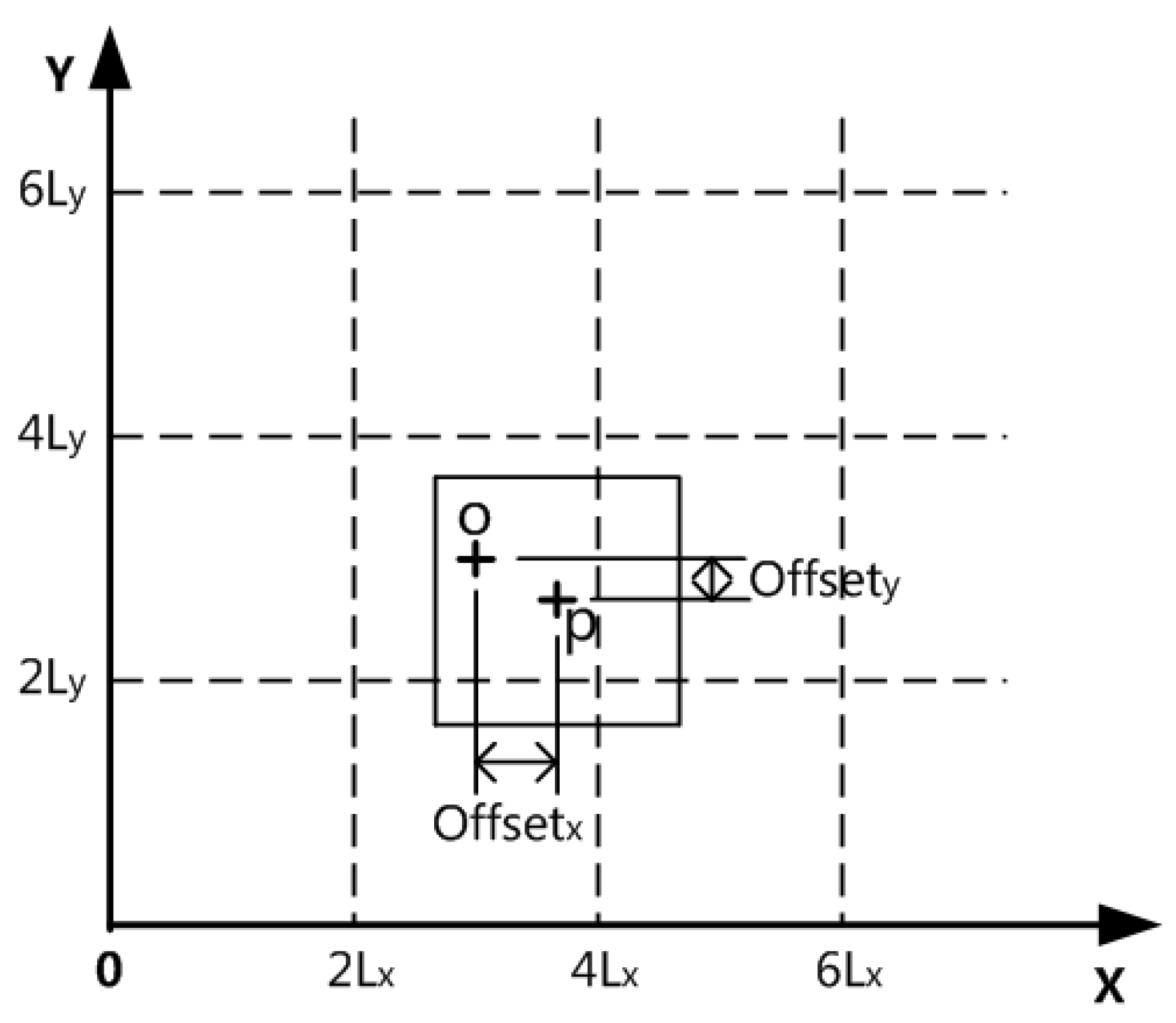
Figure 3 depicts the reference graph obtained through the original contribution algo-rithm.The contribution formula of data point
P to a grid is as follows:
In Equation (2),
denotes the contribution of data point
P to the grid,
denotes the dimension index of the dataset being processed, and
denotes the component of the contribution sought on dimension
.
Equations (3) and (4), the absolute distance between the data point P and the grid’s center point O, is represented by the term, while denotes the width of the grid in the number -dimension. represents the number of the calculated grid in the -dimension, and represents the number of the grid where the data point P is located in the -dimension.
- (2)
Improved calculation method of contribution
The improved data point
P contribution formula to a grid is as follows:
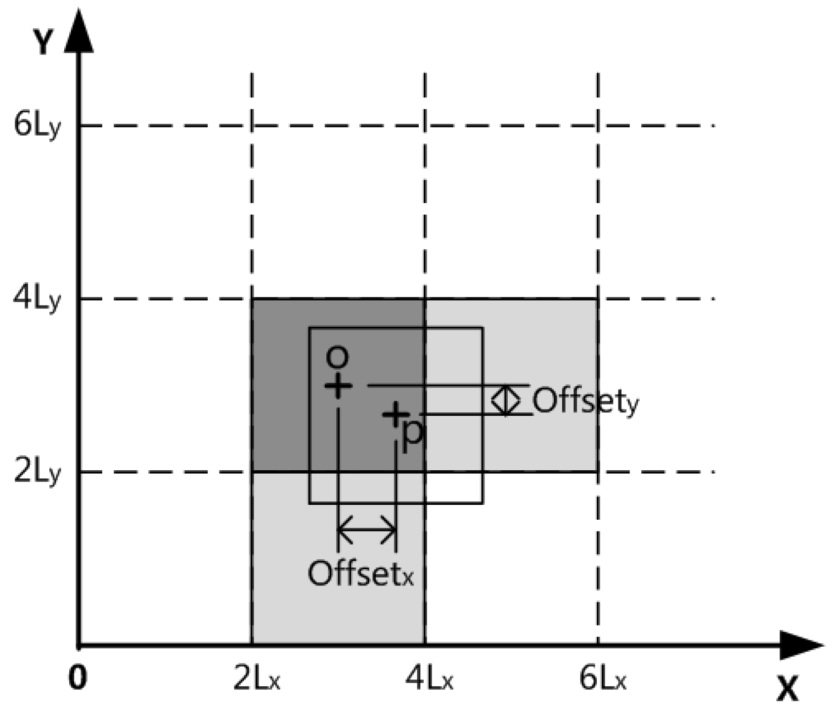
Figure 4 shows the contribution of data point
P to the grid affected by the two-dimensional space. After the improvement, the number of grids that can be affected by the data point
P is reduced to
(i.e., three, because
= 2 here), namely, the grid CubeX where the data point
P is located, i.e., the gray cross-line grid in the center of
Figure 4, and the other two related grid units CubeI sharing a connection surface with the grid unit CubeX in the
-dimensional space,
. e., the two gray grids in
Figure 4. The corresponding contribution calculation is realized by Equations (5) and (6), especially when
, all
.
3.5. Grid Density and Its Improvement
The cumulative grid contribution is often used as the grid density in the traditional contribution-based approach.
Definition 6.
(Grid’s cumulative contribution) The cumulative contribution of this grid is the total of all contributions made by the data points in both this grid and the grid that is next to it.
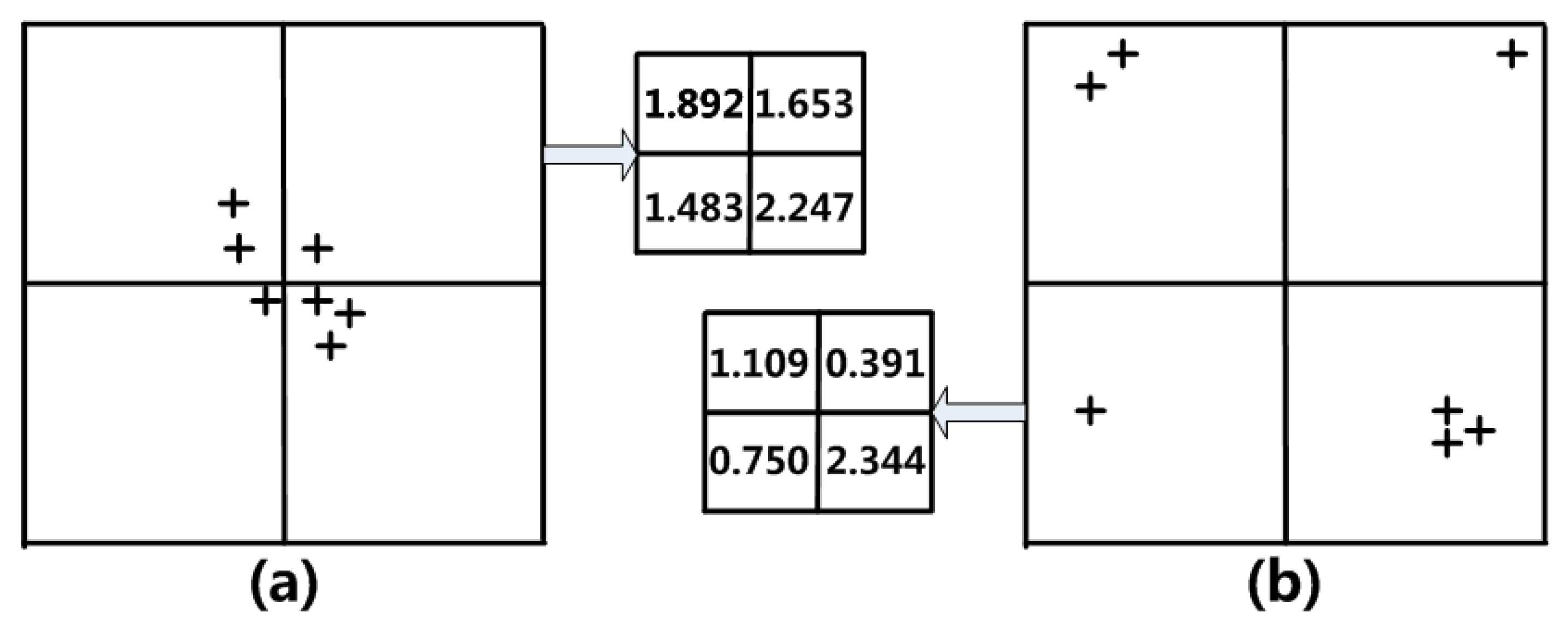
In the conventional algorithm, the grid density is calculated by the grid cumulative contribution method in
Figure 5, which is effectively compared with the example in
Figure 2. It can be seen that the “unfortunate” data points in
Figure 5a are cut apart by grids because the mutual influence of each other’s contribution does not lead to the disparity in grid density; in
Figure 5b, the data points and noise points are shown through the cumulative contribution of the grid. Therefore, in order to more properly portray the actual distribution of data points in the grid, the cumulative contribution as the grid density should be used.
The following describes an improved method of grid density calculation:
In the conventional algorithm based on contribution, the density of grid cells is completed by the “cumulative contribution”. However, this is not appropriate for clustering analysis of data stream. In the concept of “cumulative contribution”, the density of grid elements only increases and does not decrease, especially those high-density grids that are likely to remain “promoters” of clustering. Therefore, the timeliness of data should be emphasized in data stream clustering, and the contribution of old data to the grid should be gradually weakened. Therefore, this algorithm is improved by using a “gradual forgetting” approach to calculate the density of grid elements.
In this algorithm, a fixed-size time window is used to process the data stream. Each time passing a time window, this algorithm updates the original grid density by attenuation. The new density is calculated by the method shown in Equation (7).
where
is the total density of a grid unit at the
T time window,
is the cumulative contribution change brought by the new data points owned by the
T time window,
is the attenuation rate, and
is the total density of the grid unit at the time window of
T − 1. This attenuation update operation is also conducive to removing the impact of accidental events on data stream clustering.
To accurately distinguish dense and sparse grids, an accurate density threshold must be set first. Referring to some studies, the non-empty grid can be sorted according to its density from small to large, and the grid density at the first density surge is selected as the threshold, which is a more conservative selection scheme. If the prior knowledge can be used to determine the noise rate of the data set, the number of data points can be accumulated based on density sorting, and the density at the surge near the total number of noise points can be selected as the threshold, which is more accurate.
3.6. Migration Factor and Its Improvement
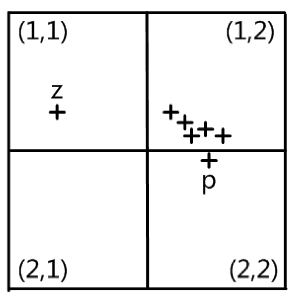
Despite being precise and efficient, the grid density estimation technique based on cumulative contribution may also confuse a few boundary points with noise points in some adverse situations, resulting in a decline in clustering quality. In the extreme cases shown in
Figure 6, the contribution to the grids (1, 1) and (2, 2) is comparable owing to the approximate symmetry of the spatial positions of the intra-class data points, and the boundary data point
P’s contribution to the grid (1, 1) is minimal due to its proximity to the boundary line. In addition, the noise point Z makes a significant contribution to the grid (2, 2) due to its proximity to the grid’s center. In conclusion, the boundary points indicated above are misclassified as noise points because the density of the noise point grid is similar to or even slightly greater than that of the boundary point grid. As a result, the migration factor in this technique will treat the border points in sparse grids appropriately.
- (1)
Original calculation method of migration factor
Definition 7. (migration factor QY) For data points in sparse grids, the determination coefficient of whether it is necessary to move them from the grid to the adjacent grid is the migration factor. The migration factor’s range of values is [0,1], and the closer it is to 1, the more often data points are requested to be relocated to neighboring grids. The data point has a component for the migration factor on each dimension. The migration factoron the i-dimension is determined as: In Equation (8), —contribution of data point to adjacent grid element on the i-dimension,
—contribution of data point to local grid element on the i-dimension.
B—is a Boolean quantity whose value is 0 or 1.
In Equation (8),
represents the precondition for the migration of data points. Specifically, when the data point is located in a sparse grid and the migration’s nearby grid is a dense grid,
is 1, otherwise, it is 0. The fraction ratio in the formula denotes the proportion of the data point’s contribution to the grid in a particular dimension to its contribution to the neighboring grid. The closer the spatial distribution of the data point is to the grid border, the higher the ratio. In the extreme cases of
Figure 6, it is simple to estimate that boundary point
P has a high migration factor
QYi, which is significantly different from the noise point
Z.
Data points are mapped in the relevant neighboring dense grid when their migration factor exceeds the migration threshold for a certain dimension, that is, the data point is “loaded” into the matching dense grid, but the computation procedure does not affect the data point’s spatial coordinates, which is the migration operation of the data point.
- (2)
Improved calculation method of migration factor
The improved calculation formula is:
In Equation (9) A′-The contribution of data points to adjacent dense grid element, is a new Boolean quantity whose value is 0 or 1.
It is the condition that determines whether a data point migrates in the data stream clustering analysis, that is, when a data point in a sparse grid is impacted by a dense grid next to it on dimension , the value is 1, otherwise, it is 0. Similarly, when the migration factor of a data point on dimension is greater than the set migration threshold, the data point is migrated.
In this algorithm, two new important pieces of information added to the grid data information mentioned earlier in the introduction, namely the value and the pointer list of migrating dense grids, are usually used together. In the migration analysis, we traverse each dense grid, set the of the data points in the adjacent sparse grid affected by it on the -dimension to 1, and add the pointer of the dense grid to the pointer list of the migrated dense grid.
If a data point’s migration factor to many adjacent dense grids exceeds the migration threshold in data stream clustering analysis, this data point is mapped into the corresponding multiple adjacent dense grids. It will be put into the cluster found first in accordance with the principle of “whoever finds it first gets it”.
3.7. The Process of MDDSDB-GC
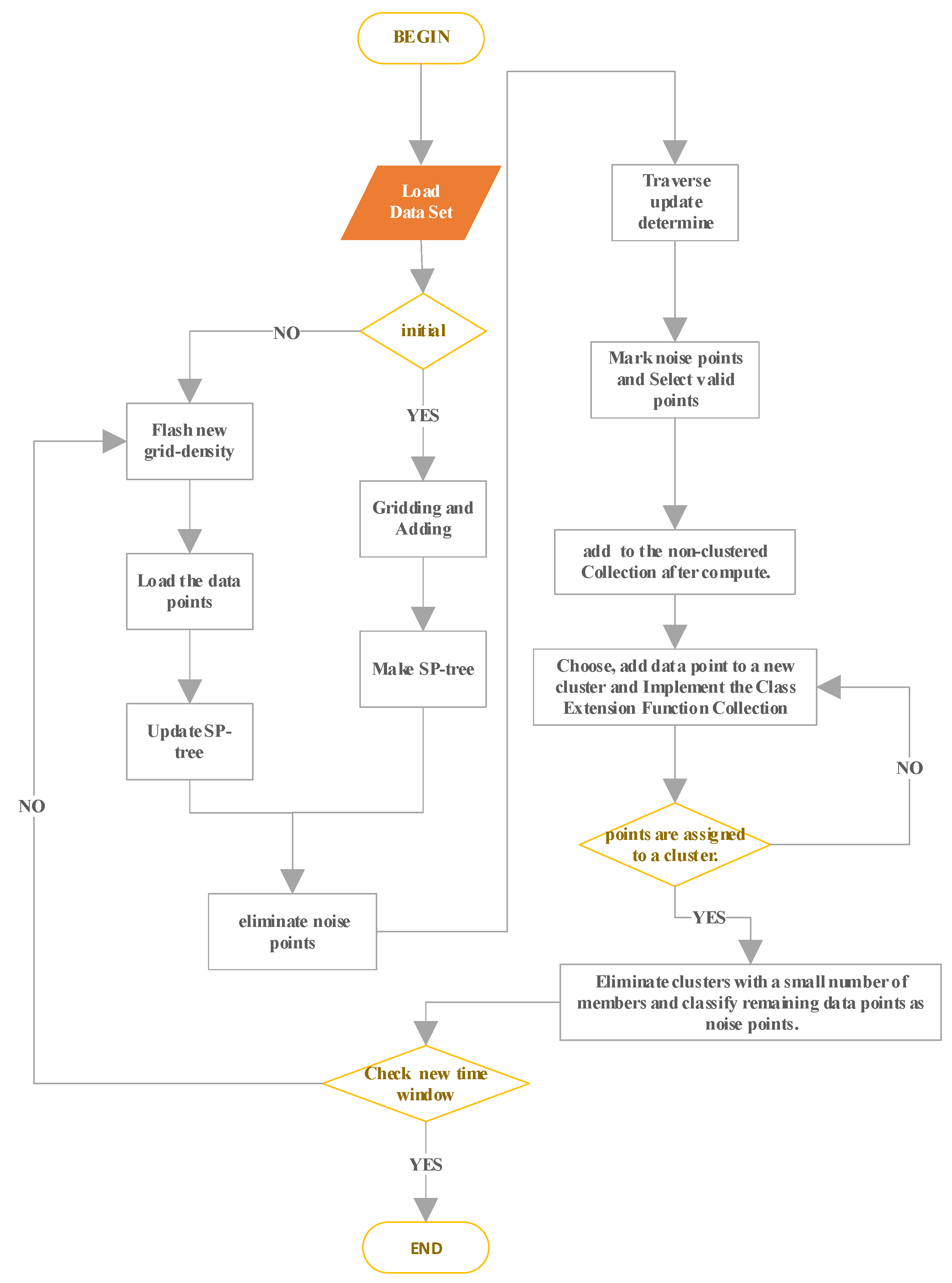
The algorithm’s steps are thoroughly explained below to ensure its completeness and practicality. A detailed flow chart is provided in
Figure 7 to enhance understanding of the algorithm’s execution process.
- (1)
Load the data set in the new time window and judge whether the initialization process is necessary. If so, go to the second step. If not, go to the fourth step. It should be noted that the initialization process is only carried out when the data set in the first time window is loaded. At this time, the grid has not been divided and the SP-tree has not been established.
- (2)
Gridding the standardized new data set and adding the data points to the appropriate grid.
- (3)
Make a SP-tree sp-tree-grid that corresponds to a non-empty grid and move to step 7.
- (4)
With the SP-tree sp-tree-grid, the cumulative contribution of all non-empty grids is multiplied by the attenuation rate to form a new grid density.
- (5)
Load the data points in the new dataset into the corresponding grid.
- (6)
Update SP-tree sp-tree-grid.
- (7)
Identify and eliminate noise points by distinguishing dense grids. The cumulative contribution of non-empty grids is sorted by traversing the sp-tree sp-grid, and the appropriate density threshold is selected based on prior knowledge. At the same time, the SP-tree sp-tree-dense of the dense grid and the SP-tree sp-tree-sparse of the sparse grid is created.
- (8)
Traversing each dense grid corresponding to the SP-tree sp-tree-dense of dense grids, updating the data information in the adjacent sparse grids affected on the i-dimensional, setting the newistrue of the data points in this grid to 1, and adding the dense grid pointer to the pointer list of migrating dense grids.
- (9)
The migration factors of data points in all sparse grids are determined using SP-tree sp-tree-sparse. When the migration factor exceeds the set threshold, the corresponding migration operation is performed and the sp-tree-dense is updated.
- (10)
Traversing SP-tree sp-tree-sparse, the remaining data points in the sparse grid are temporarily marked as noise points.
- (11)
SP-tree for selecting valid data points: sp-tree-cluster. For the original data set with noise points, sp-tree-dense is used as the SP-tree of effective data points; for the original data set without noise points, sp-tree-grid is used as the SP-tree of effective data points.
- (12)
With the help of SP-tree sp-tree-cluster, the k nearest data point sets
Np of each valid data point
P are searched and determined, and then the average distance value, denoted by the abbreviation “
” of valid data point
P is computed.
- (13)
Include in the non-clustered data point collection W all of the valid data points P.
- (14)
Choose the data point M from W that has the least value and do the following actions:
- a.
Give data point M a fresh cluster identifier Ci, that is, point M becomes a member of the new class Ci.
- b.
Remove data point M from W.
- c.
Setting the average distance inside the original cluster Ci ’s cluster
- d.
Call class extension function collection (Ci, M)
- (15)
Implementation of Class Extension Function Collection (Ci, M).
For any data point Q in the k nearest dataset of data point M, if the data point Q is in the queue list and () at the same time, operate as follows:
- a.
Add data point Q to cluster Ci
- b.
Remove data point Q from W
- c.
Update the average distance within a cluster of cluster Ci
- d.
Call class extension function collection (Ci, Q)
According to the equation above (), the parameter var is a distance threshold parameter whose value should be greater than 1 and set by the user according to the actual situation. The closer to 1, the closer to the DST value of the data point in the cluster is required, that is, the stricter the access condition of the cluster is. Therefore, parameter var aggregates data into different categories from the perspective of spatial density. In Equation (12), Ni is the number of members in cluster Ci after adding the data point Q to cluster Ci.
- (16)
Repeat steps 14 and 15 until the non-clustered dataset W is cleared.
- (17)
Eliminate clusters with a small number of members and classify the data points into noise points.
- (18)
To determine whether there is a new time window or not, turn to step 4.
- (19)
The whole clustering process ends.
4. Experimental Validation
4.1. Effectiveness Verification of MDDSDB-GC Algorithm
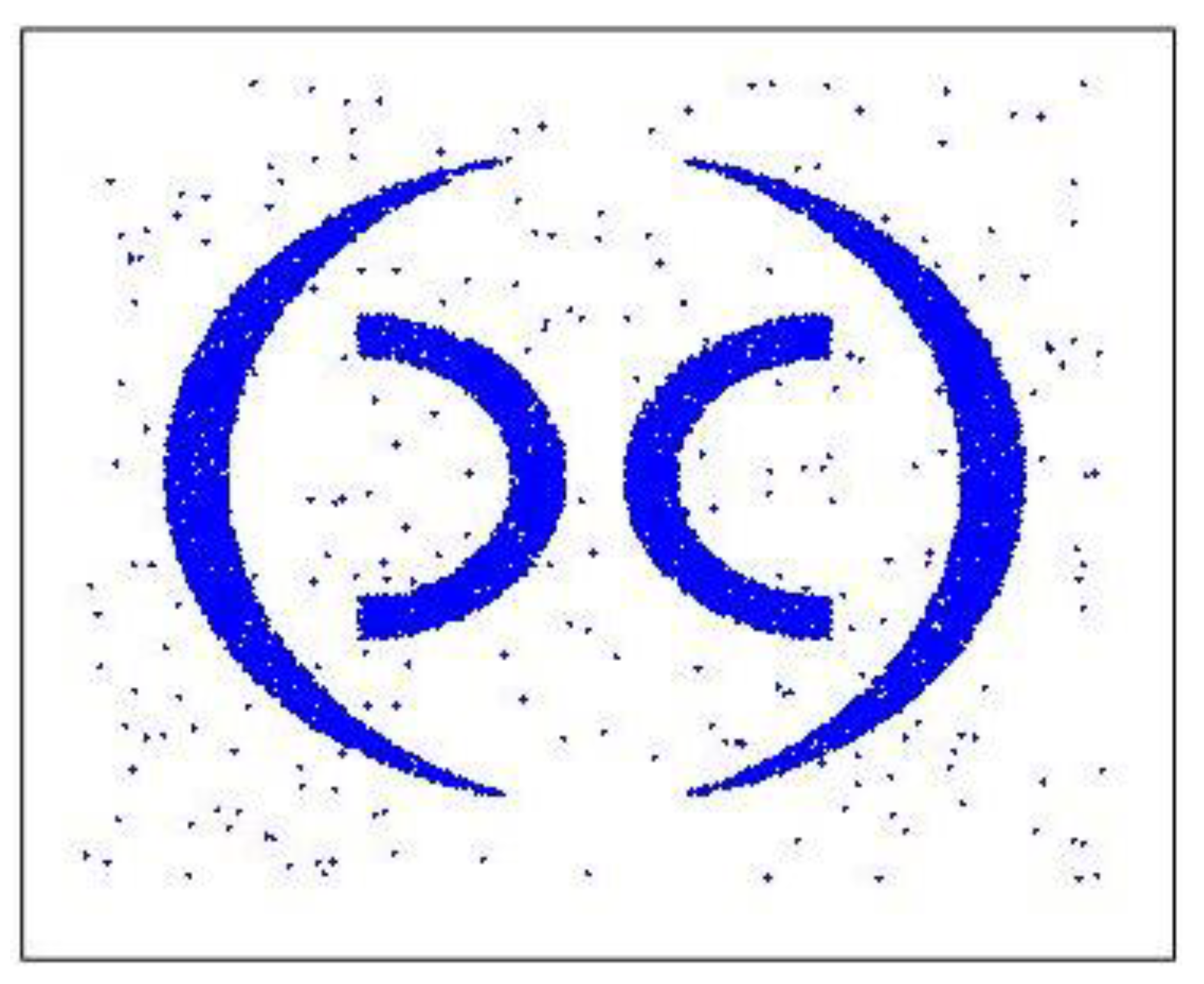
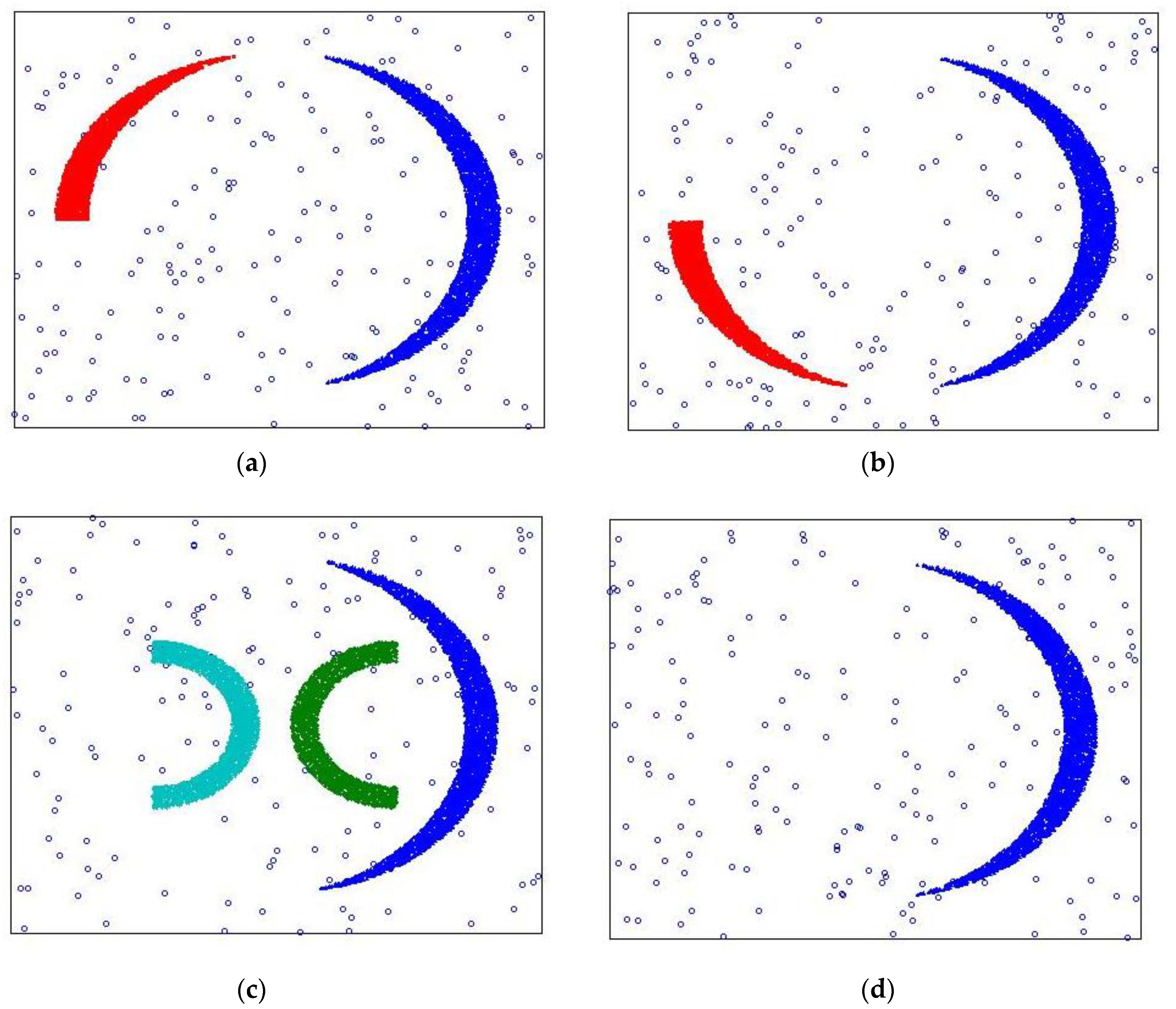
After completing the expansion and improvement of the MDDSDB-GC algorithm, the effectiveness of the algorithm is verified. This verification adopts the experimental method of clustering analysis of standard (data stream) data set 1 and makes a judgment through the actual clustering results. To effectively reflect the dynamic change of clustering, the time sequence of clustering in standard data set 1 is adjusted to make the clustering dynamic change. Its change process includes the drift of the cluster, the emergence of new clusters, and the disappearance of old clusters.
In this experiment, the MDDSDB-GC algorithm divides the x-axis and y-axis into 30 segments, namely, the whole space is divided into 900 grids. Divided into 6 fixed time windows, each fixed time window contains 80,000 data points. Load 80,000 data points of first-time window while initialization with attenuation rate as 0.7. Therefore, after six time windows, data stream clustering analysis is completed.
Compare with the original data in
Figure 8,
Figure 9a–d display the experimental results. it can be seen that the clustering results are correct, the change of the class is also correctly expressed, and the clustering accuracy is also high, which proves the effectiveness of the MDDSDB-GC data stream clustering algorithm.
4.2. Time Complexity Analysis of MDDB-GC Algorithm
The time complexity analysis of the MDDB-GC algorithm is carried out. The pre-foundation of the MDDB-GC algorithm is d-dimensional (data stream) data set S, which contains N data points and is divided into k time windows. The grid is divided into L segments on each dimension, and then there are grids.
In each time window of the MDDB-GC algorithm, the time complexity is O (N) in the grid division and data binning stage. In building an SP tree, calculating cumulative contribution, dividing a dense grid, calculating migration factor and migration action, the time complexity is O (G); in the clustering action stage, the time complexity is O (g2), where g is the number of data points in the SP-tree index grid of effective data points. In summary, in all time windows, the total time complexity of the algorithm is O (kg2), which is further simplified, and the total time complexity is about O (g2).
The original multi-density DBSCAN algorithm, in contrast, has a temporal complexity of around O (N2), where N is the number of core data points. Since g is considerably smaller than N, the time of the MDB-GC algorithm is much shorter than that of the original multi-density DBSCAN algorithm, and the performance is better.
4.3. Experimental Results of the MDDSDB-GC Algorithm
In this experiment, taking into account the characteristics of the MDDSDB-GC algorithm, that is, the time complexity of the algorithm is associated with the amount of data points g in the SP-tree index grid of the effective data point, that is, two different datasets with the same amount of data, because of the different spatial distribution, it will lead to the different number of SP-tree index grids of the effective data point, and then the clustering time of the MDDB-GC algorithm is also different.
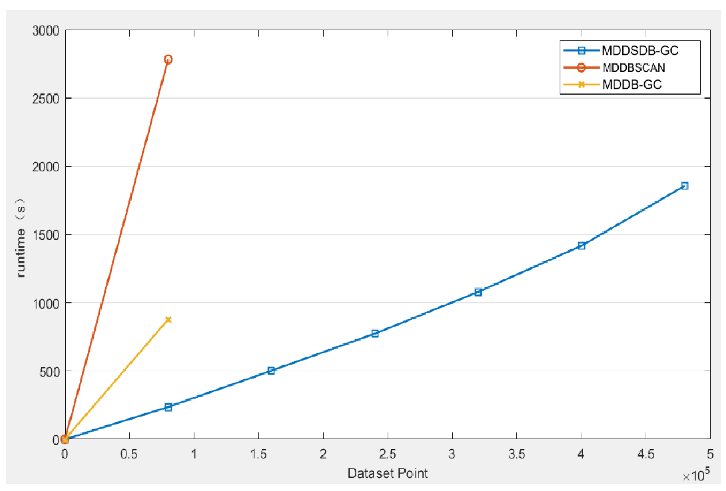
The above figure (
Figure 10) is the comparison of the runtime required for the three algorithms to complete the experimental data set. It is evident that that only the MDDB-GC algorithm can deal with data stream and large datasets, so MDDB-GC and MD-DBSCAN cannot deal with the data in the later five time windows. In the runtime, the MDSDB-GC algorithm is significantly superior. It can be found that the MDSDB-GC algorithm has more advantages in processing high-dimensional data sets than MDDB-GC and MD-DBSCAN.
