Expanding Measuring Range of LWD Resistivity Instrument in High Permittivity Layers

Abstract

The effective measuring range of an electromagnetic wave resistivity instrument used in logging while drilling (LWD) is small, and the resistivity measurement is greatly influenced by the dielectric constant, especially in high-dielectric-constant formations. In this paper, the response characteristics of the instrument under a high dielectric constant are investigated by a numerical simulation algorithm, and the resistivity conversion method is determined. The results show that the higher the working frequency of the electromagnetic wave resistivity instrument while drilling, and the greater the formation of background resistivity, the greater the influence of the dielectric constant on the logging response. The existence of the dielectric constant will cause the phase shift and amplitude attenuation of the measured signal to migrate, and this migration is proportional to the formation resistivity and the dielectric constant. According to this rule, the resistivity–permittivity response library is established, and the formation permittivity is calculated by the inversion of the library. On the basis of obtaining the formation permittivity, the migration of the logging signal permittivity is corrected, the influence of the dielectric constant is eliminated, and the measuring precision and measuring range of the instrument in the high-dielectric-constant formation are enlarged.

1. Introduction

With the extensive application of complex drilling techniques, such as highly deviated wells, horizontal wells, and multilateral wells [1], as well as the high complexity and concealment of oil and gas reservoirs, logging evaluation is facing new difficulties and challenges [2]. The measuring points of the resistivity instrument in LWD (logging while drilling) are less affected by mud invasion because of the short drilling time [3,4]. The resistivity data in LWD can reflect the real formation parameters and provide logging curves for different detection depths. Therefore, the instrument in LWD has a broad application prospect. In recent years, the technology of electromagnetic wave logging while drilling provided an effective way to solve these difficulties, with its real-time efficient geological guidance and reservoir evaluation functions. Electromagnetic wave resistivity instruments and the associated data-processing technology have become inevitable requirements for the rapid development of logging-while-drilling technology. Three oil service companies Schlumberger, Halliburton, and Baker Hughes, each have their own series of the electromagnetic wave resistivity instrument for use during drilling [5,6,7]. To satisfy the demands of geological guiding, they have successively launched azimuth electromagnetic wave resistivity instruments while drilling Periscope, ADR, and APR, all of which have the capacity to identify formation boundaries and real-time boundaries [8,9,10]. With the wide application of drilling technology in horizontal wells and highly deviated wells, the application of cable logging is restricted to a certain extent. Logging data acquisition is widely carried out while drilling, and electromagnetic wave resistivity measurement while drilling has become the development trend for underground resistivity measurement.

The electromagnetic wave resistivity instrument used in LWD transmits a certain frequency of electromagnetic wave signals via a transmitting coil, and uses the two receiving coils at different distances from the emitter in order to obtain the phase shift and amplitude attenuation changes of the induced electromagnetic wave and describe the formation resistivity [5,6,7]. However, the amplitude resistivity cannot reflect the true resistivity of high-resistance formations [8]. Generally, the traditional method is to use the dielectric constant plate method to calibrate the measured resistivity, because the dielectric constant is obtained through empirical formulas and contains errors [9,10,11,12,13]. Correction is only effective when the influence of the dielectric constant is small [14,15]. When the measured value exceeds the range of the resistivity conversion table, due to the influence of the relative dielectric constant, the formation resistivity cannot be obtained [16,17,18]. Correction of the relative dielectric constant usually uses a relative dielectric constant correction chart, which provides only a limited-range correction of the conversion resistivity, rather than addressing the impact of the dielectric constant on the source measurement response [19,20,21].

Aiming at the influence of the formation dielectric constant on logging response, this paper proposes a numerical simulation algorithm based on electromagnetic wave resistivity in LWD. This algorithm provides the characteristics of high accuracy and fast correction. The influence of the dielectric constant on logging signal response is studied through numerical simulation, and its laws are summarized. A fast correction function formula for the resistivity and dielectric constant is established. The measured information is used to quickly invert the dielectric constant. Under the condition of obtaining the formation dielectric constant, a numerical simulation algorithm is used to calculate the phase shift and amplitude attenuation offset caused by the dielectric constant, and the acquired signal is offset corrected, thereby eliminating the impact of the formation dielectric constant on the logging response during the data acquisition phase. This method can effectively eliminate the influence of the dielectric constant and improve measurement accuracy, allowing the resistivity measurement range of the instrument to be expanded. Therefore, it solves the defect that the resistivity measurement error of the high-dielectric-constant formation instrument is too large, making it difficult, or even impossible, to measure, and has practical application value.

2. Materials and Methods

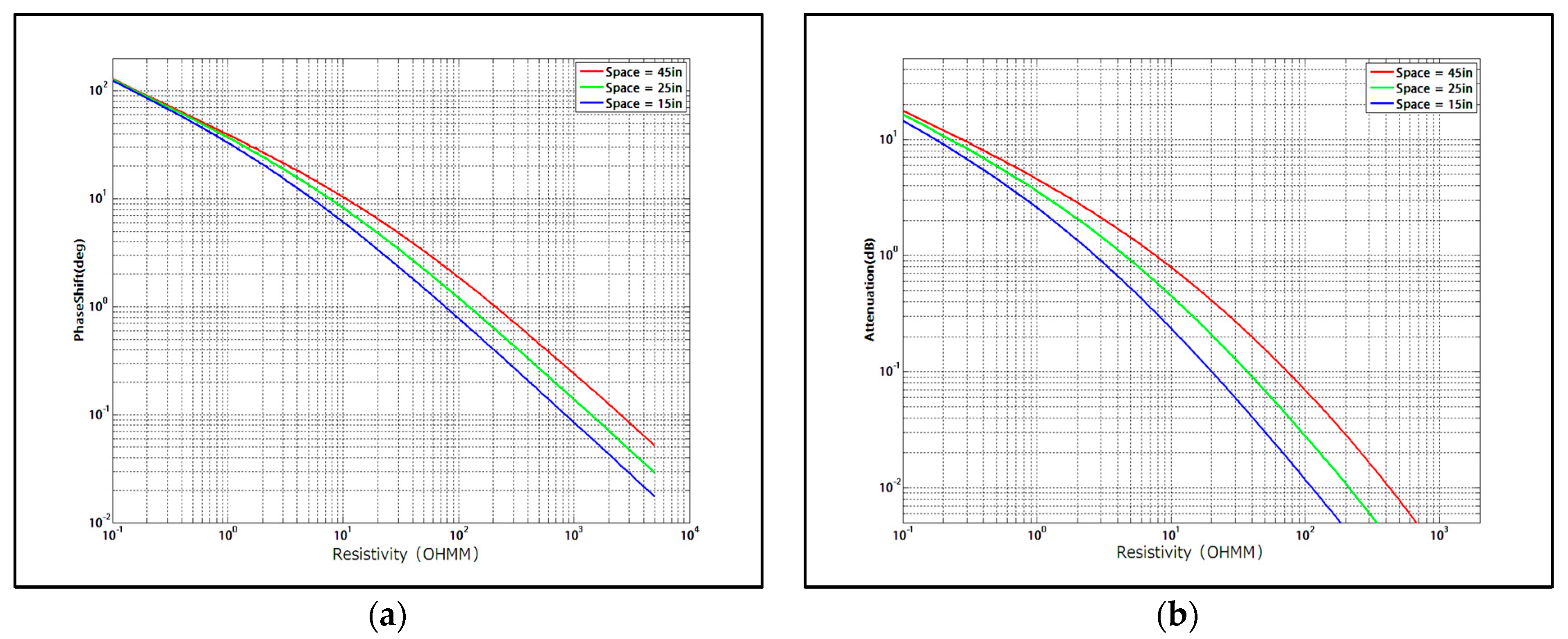
2.1. Mathematical Model of Numerical Simulation of Electromagnetic Wave Resistivity in LWD

Based on the Maxwell Equation [11], the electromagnetic field in electromagnetic wave logging while drilling satisfies Maxwell equations:

$$\nabla \times \mathrm{E}=-\mathrm{i}\mathsf{\omega }\mathsf{\mu }\mathrm{H}$$

(1)

$$\nabla \times \mathrm{H}=\mathsf{\sigma }\mathrm{E}+\mathrm{J}$$

(2)

where $\mathrm{E}$ represents electric field intensity, $\mathrm{H}$ represents magnetic field intensity, $\mathrm{J}$ represents source current density, $\mathsf{\omega }$ represents source current angular frequency, $\mathsf{\sigma }$ represents conductivity, and $\mathsf{\mu }$ represents permeability.

$$\nabla \times \nabla \times \mathrm{E}-{\mathsf{\omega }}^2\mathsf{\mu }{\mathsf{\epsilon }}_{\mathrm{c}}\mathrm{E}=-\mathrm{j}\mathsf{\omega }\mathsf{\mu }\mathrm{J}$$

(3)

Here, ${\mathsf{\epsilon }}_{\mathrm{c}}=\mathsf{\epsilon }-\frac{\mathrm{i}\mathsf{\sigma }}{\mathsf{\omega }}$ represents complex permittivity and $\mathsf{\epsilon }={\mathsf{\epsilon }}_{\mathrm{r}}{\mathsf{\epsilon }}_0$, in which ${\mathsf{\epsilon }}_0$ represents vacuum permittivity and ${\mathsf{\epsilon }}_{\mathrm{r}}$ represents relative permittivity.

Consider:

$$\mathrm{\nabla }\mathrm{E}={\mathrm{E}}_{\mathrm{p}}+{\mathrm{E}}_{\mathrm{s}}$$

(4)

Here, the background field ${\mathrm{E}}_{\mathrm{p}}$ is the electric field when the entire space is filled with a medium having a conductivity of ${\mathsf{\sigma }}_0$, which satisfies the equation:

$$\nabla \times \nabla \times {\mathrm{E}}_{\mathrm{p}}-{\mathsf{\omega }}^2\mathsf{\mu }{\mathsf{\epsilon }}_{\mathrm{c}0}{\mathrm{E}}_{\mathrm{p}}=-\mathrm{j}\mathsf{\omega }\mathsf{\mu }\mathrm{J}$$

(5)

Here, ${\mathsf{\epsilon }}_{\mathrm{c}0}=\mathsf{\epsilon }-\frac{\mathrm{i}{\mathsf{\sigma }}_0}{\mathsf{\omega }}$. Subtracting Equation (5) from Equation (3) and using Equation (4), we can obtain:

$$\nabla \times \nabla \times {\mathrm{E}}_{\mathrm{s}}-{\mathsf{\omega }}^2\mathsf{\mu }\mathsf{\epsilon }{\mathrm{E}}_{\mathrm{s}}={\mathsf{\omega }}^2\mathsf{\mu }(\mathsf{\epsilon }-{\mathsf{\epsilon }}_{\mathrm{c}0}){\mathrm{E}}_{\mathrm{p}},$$

(6)

where the background field is calculated by analytical method and the secondary field is calculated by finite element method. Compared with Equation (3), the solution of Equation (6) changes smoothly and can be solved by sparse grids, which reduces the calculation workload.

If a large enough area is selected to attenuate the electric field on the boundary to approximately 0, Equation (6) only needs to satisfy the boundary condition:

$$\mathrm{n}\times \mathrm{E}|\partial \mathsf{\Omega }=0$$

(7)

Here, $\partial \mathsf{\Omega }$ is the boundary of $\mathsf{\Omega }$ the interested area, and $\mathrm{n}$ is its normal direction.

Considering the boundary condition of Equation (7), the vector wave Equation (6) is transformed into its weak product form:

$${\int }_{\mathsf{\Omega }}^{}\nabla \times {\mathrm{E}}_{\mathrm{s}}·\nabla \times \mathrm{N}\mathrm{d}\mathrm{V}-{\int }_{\mathsf{\Omega }}^{}{\mathsf{\omega }}^2\mathsf{\mu }\mathsf{\epsilon }{\mathrm{E}}_{\mathrm{s}}·\mathrm{N}\mathrm{d}\mathrm{V}={\int }_{\mathsf{\Omega }}^{}{\mathsf{\omega }}^2\mathsf{\mu }(\mathsf{\epsilon }-{\mathsf{\epsilon }}_{\mathrm{c}0}){\mathrm{E}}_{\mathrm{p}}·\mathrm{N}\mathrm{d}\mathrm{V}$$

(8)

Here, $\mathrm{N}$ is a vector primary function. The electric field value of each edge can be obtained by solving Equation (8) using the vector edge finite element method. By integrating each side of the receiving coil, the induced voltage of the receiving coil can be obtained.

2.2. Investigation on the Influence Rule of Permittivity and Resistivity

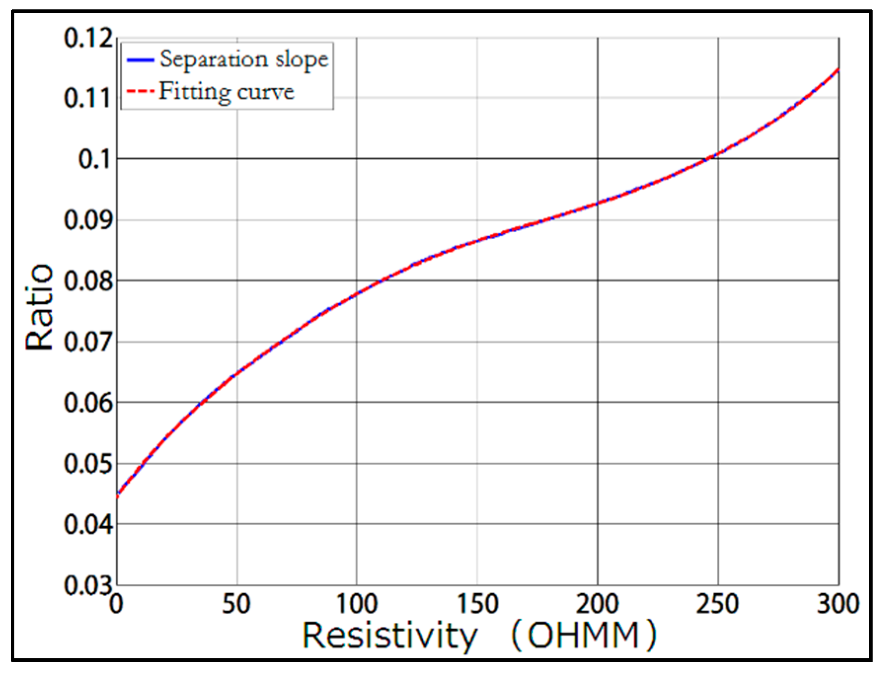
2.2.1. Resistivity Conversion Method

Figure 1a,b describe the relationship between induced voltage and resistivity in a uniform infinite thickness formation. Without considering the impact of drilling and mud, and with the distance between the two receiving coils fixed at 6 inches, the distance from the transmitting coil to the midpoint of the two receiving coils is considered to vary, and may be 9 inches, 15 inches, 27 inches, or 39 inches. The operating frequency is set to 2 MHz, and the formation resistivity ranges from 0.1 ohm.m–10,000 ohm.m.

In Figure 1a,b, the non-monotonic characteristic of the relationship between the measured coil voltage and the formation resistivity is obvious, and it is not suitable to use the voltage variation to measure the formation resistivity value. The transmitting coil transmits an electromagnetic wave signal, and the electromagnetic wave attenuates in the propagation process. The amplitude and phase received by the near and far coils are different. The formulas for calculating the phase shift and amplitude attenuation at the two receiving coils are shown in Equations (9) and (10), respectively:

$$\mathrm{P}\mathrm{H}\mathrm{S}={\tan }^{-1}\frac{\mathrm{I}\mathrm{m}\left({\mathrm{V}}_{\mathrm{R}1}\right)}{\mathrm{R}\mathrm{e}\left({\mathrm{V}}_{\mathrm{R}1}\right)}-{\tan }^{-1}\frac{\mathrm{I}\mathrm{m}\left({\mathrm{V}}_{\mathrm{R}2}\right)}{\mathrm{R}\mathrm{e}\left({\mathrm{V}}_{\mathrm{R}2}\right)}$$

(9)

$$\mathrm{A}\mathrm{R}\mathrm{S}=20\log \left(\frac{{\left(\mathrm{I}\mathrm{m}\right({\mathrm{V}}_{\mathrm{R}1}\left)\right)}^2+{\left(\mathrm{R}\mathrm{e}\right({\mathrm{V}}_{\mathrm{R}1}\left)\right)}^2}{{\left(\mathrm{I}\mathrm{m}\right({\mathrm{V}}_{\mathrm{R}2})}^2+{\left(\mathrm{R}\mathrm{e}\right({\mathrm{V}}_{\mathrm{R}2}\left)\right)}^2}\right)$$

(10)

Due to the transmission coil emitting electromagnetic wave signals of a specific frequency, any change in formation resistivity will lead to different propagation speeds of electromagnetic waves within the formation. This, in turn, affects the amplitude attenuation of electromagnetic waves and the phase shift between different coils. Figure 2a illustrates the correlation between resistivity and phase shift, while Figure 2b illustrates the relationship between resistance and amplitude attenuation.

Figure 2a,b show the formation resistivity on the lateral axis and the phase shift or amplitude attenuation on the vertical axis. Different curves show the resistivity–phase shift correspondence and the resistivity–amplitude attenuation correspondence when the transmitting coils are at different distances from the midpoint of the two receiving coils. The distance between the two receiving coils is fixed at 6 in. As can be observed from Figure 2a,b, resistivity and phase shift, as well as resistivity and amplitude attenuation, are in one-to-one correspondence, and the phase shift and amplitude attenuation decrease monotonically with the change in resistivity. Because the phase shift and amplitude attenuation have this property, the phase shift and amplitude attenuation corresponding to the induced electromotive force obtained by the receiving coil in actual measurement can be easily converted into a resistivity signal in combination with the above correspondence.

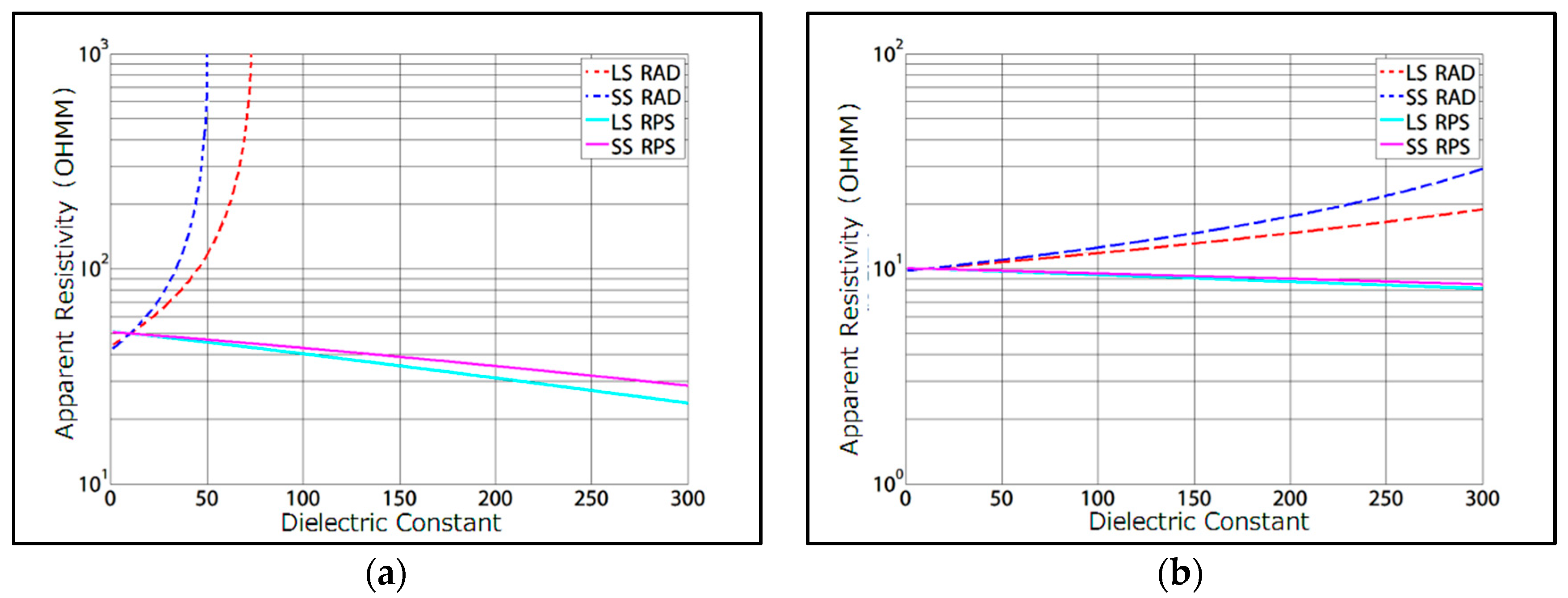
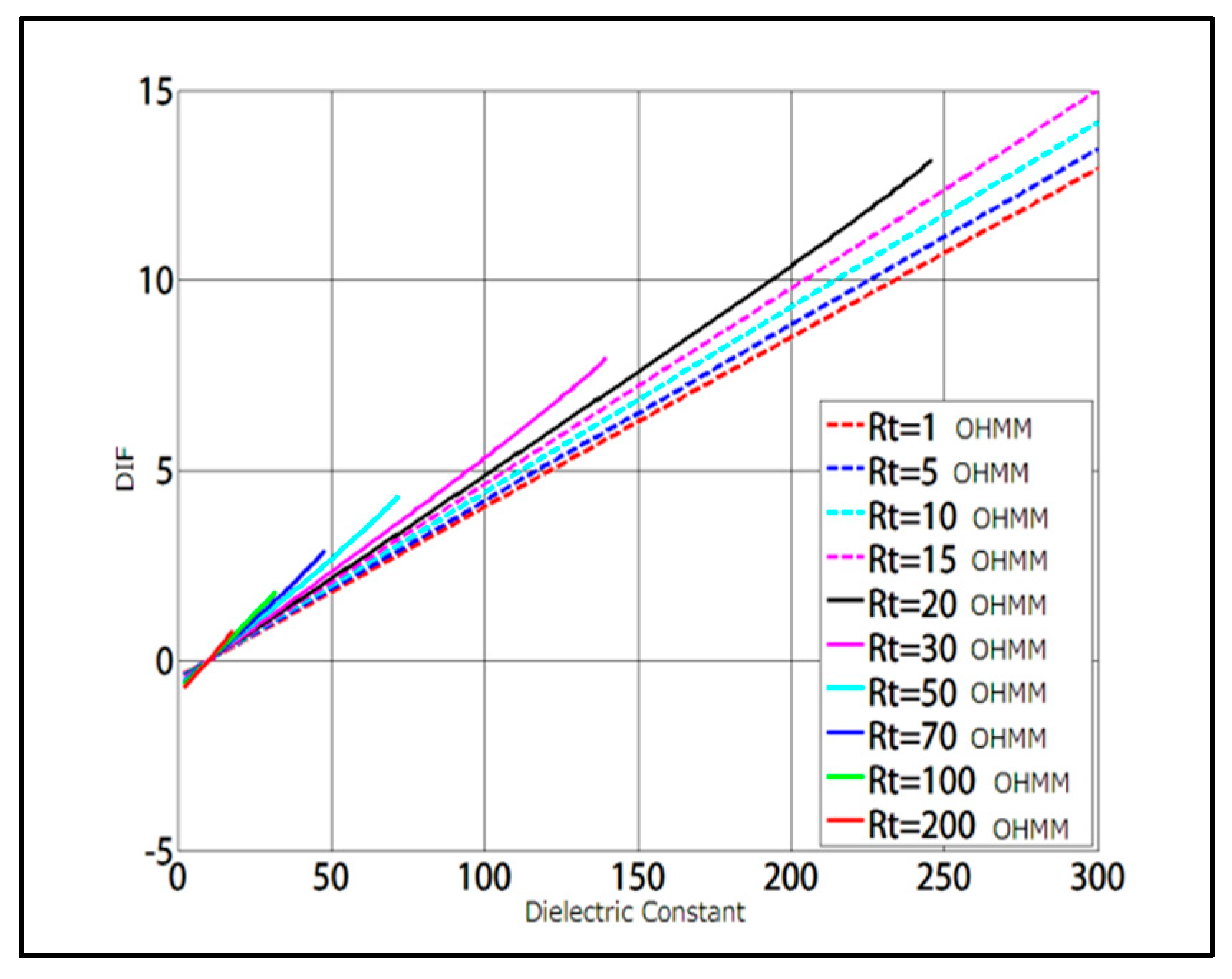
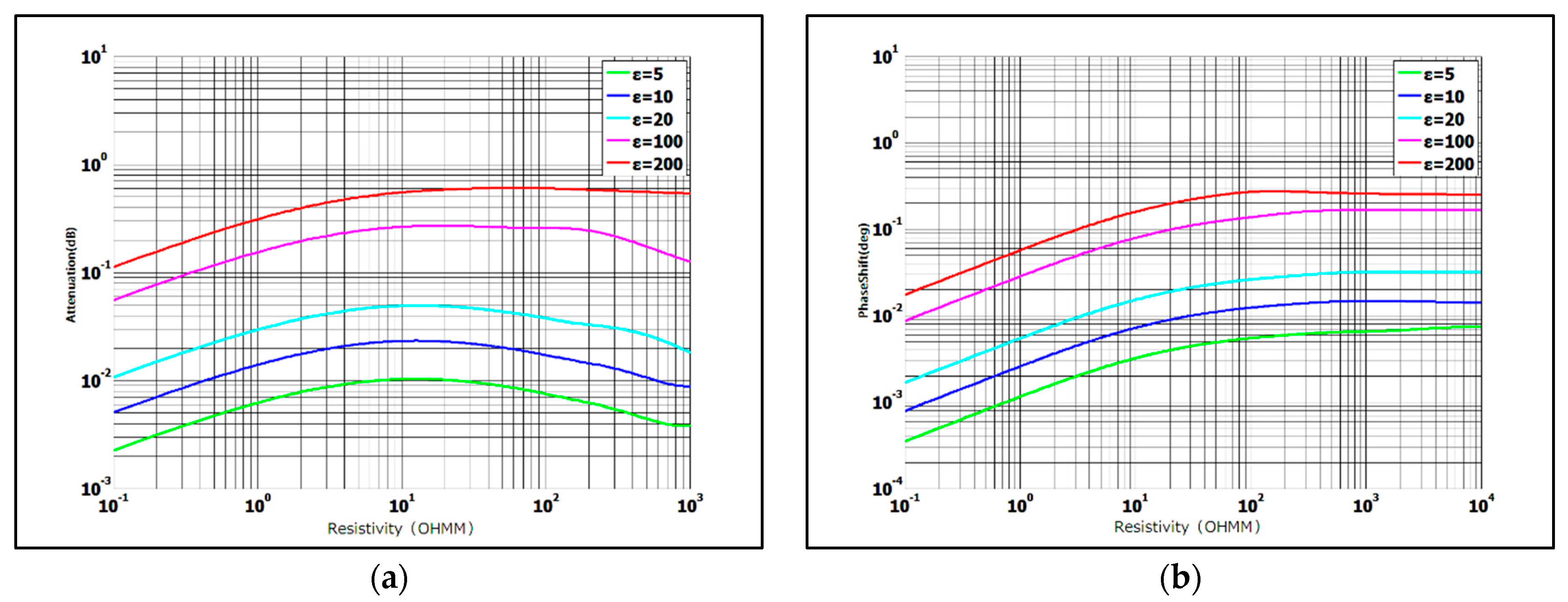
2.2.2. Influence Rules of Permittivity

The parameters of the model shown in Figure 2 have been modified and recalculated, considering formation relative dielectric constants of 1, 5, 10, 20, 100, and 200. The calculated resistivity–amplitude attenuation correspondence and resistivity–phase shift correspondence are shown in Figure 3.

As can be observes from Figure 3a, the phase shift–resistivity correspondence relationship varies greatly under different relative dielectric constants. The larger the dielectric constant, the smaller the phase shift decrease. It can be observed from Figure 3b that the amplitude attenuation–resistivity correspondence varies greatly under different relative dielectric constants. The reduction in amplitude attenuation increases with the increasing dielectric constant, even to a negative value.

From Figure 3, it is apparent that the phase shift–resistivity correspondence curves under different relative dielectric constants are essentially the same at low frequencies, as shown in Figure 3a. This indicates that the formation dielectric constant has a minimal impact on the measured values of the instrument when the frequency is low. However, only in cases of high resistance and high dielectric constant does the dielectric constant have a noticeable effect on the measured value. On the other hand, the amplitude attenuation–resistivity correspondence curves under different relative dielectric constants essentially coincide at low frequencies, as shown in Figure 3b. This suggests that the influence of the dielectric constant on the measured values of the instrument cannot be ignored in high-resistivity areas.

The resistivity conversion relationship was calculated by changing the model parameters of Figure 1, where the formation resistivity values were set to 10 ohm.m and 50 OHMM, and the formation relative dielectric constant varied from 1 to 300. The resistivity curves obtained by calculating the resistivity conversion relationship with fixed dielectric constants (RAD for resistivity amplitude, RPS for resistivity phase shift, LS for source distance of 35 in, and SS for source distance of 22 in) are shown in Figure 4. It is evident that, under fixed dielectric constants, the larger the difference between the dielectric constant and the real value, the greater the deviation between the measured value and the real value. Additionally, the higher the formation resistivity, the larger the deviation amplitude. For high resistivity formations (on the right), when the relative dielectric constant is more than a certain value (70), RAD tends toward infinity (beyond the measurement range), and even the subsequent dielectric constant correction cannot reduce the true resistivity of the layers.

3. Results

3.1. Relative Dielectric Constant Inversion

The influence of the dielectric constant on the measured value is non-linear, and increases as the dielectric constant increases. Additionally, the non-linear increment varies under different formation resistivities. Therefore, to eliminate the influence of the relative dielectric constant on the measured value, it is necessary to determine the formation relative dielectric constant value first. The variation of apparent resistivity with the dielectric constant was investigated, and the following conclusions were drawn: (1) The curve separation increases as the dielectric constant increases, and (2) different resistivities lead to different degrees of curve separation. In order to establish a rapid inversion database, layer resistivity ranging from 0.2 to 2000 OHMM and relative dielectric constant ranging from 1 to 200 OHMM were considered. The curve separation coefficient DIF was defined as follows:

$$DIF=7.5\times \frac{{(RPS-RAD)}^3}{RPS\times RAD\times log\left(\frac{RPS+RAD}{2}\right)}$$

(11)

The curves of phase difference and amplitude ratio of high frequency and long source distance are calculated under different resistivities. The variation of the separation coefficient with the relative dielectric constant is shown in Figure 4. It can be observed that the curve separation is linearly related to the relative permittivity, and the separation coefficient of the log curve corresponds to a line segment in the graph under each background resistivity value. The length of the line segment is determined by the range of resistivity measurement.

The curve corresponding to resistivity in Figure 5 separates straight lines through points where the dielectric constant is 10 and the separation coefficient is 0. Therefore, each curve can be linearly related:

$$\mathrm{y}=\mathrm{a}\mathrm{x}+\mathrm{b}$$

(12)

The straight line can be determined by determining the linear coefficient a and the offset b, and then the curve separation can be obtained through the straight line. Therefore, the linear coefficients satisfying the linear relationship under different resistivities are extracted, and the curves are fitted, as shown in Figure 6.

The inversion of the formation dielectric constant is carried out by Marquette’s least square method. Firstly, the differentiation coefficient of the curve is calculated from the logging response curve, and the least square objective function is established as follows:

$${\mathrm{m}\mathrm{i}\mathrm{n}}_{\mathrm{x}\in {\mathrm{R}}^{\mathrm{n}}}\mathrm{f}\left(\mathrm{x}\right)=\frac{1}{2}\mathrm{r}{\left(\mathrm{x}\right)}^{\mathrm{T}}\mathrm{r}\left(\mathrm{x}\right)=\frac{1}{2}{\sum }_{\mathrm{i}=1}^{\mathrm{m}}{\left[{\mathrm{r}}_{\mathrm{i}}\right(\mathrm{x}\left)\right]}^2,\mathrm{m}\ge \mathrm{n}$$

(13)

Here, r:$R^n\to R^m$ is a non-linear function of x, which is a mapping relationship between resistivity, the dielectric constant, and the differential coefficient of the logging curve; R represents an independent variable vector; m represents the number of unknown variables; and n represents the number of differentiation coefficients fitted to the forward response curve. The Jacobian matrix of the objective function is solved using the gradient method to form Jacobian linear equations, and the fastest descent direction of the objective function is calculated by solving the equations:

$$\mathrm{J}=\left(\begin{array}{ccc}\frac{\partial r_1}{\partial x_1}& \cdots & \frac{\partial r_1}{\partial x_n}\\ ⋮& \ddots & ⋮\\ \frac{\partial r_m}{\partial x_1}& \cdots & \frac{\partial r_m}{\partial x_n}\end{array}\right)$$

(14)

The gradient of the objective function is calculated according to the following formula:

$$\mathrm{g}\left(\mathrm{x}\right)={\sum }_{\mathrm{i}=1}^{\mathrm{m}}{\mathrm{r}}_{\mathrm{i}}\left(\mathrm{x}\right)\nabla {\mathrm{r}}_{\mathrm{i}}(\mathrm{x})=\mathrm{J}(\mathrm{x}{)}^{\mathrm{T}}\mathrm{r}\left(\mathrm{x}\right)$$

(15)

Here, J(x) is the Jacobian matrix of r(x), solving the objective function according to the obtained model change direction and step size, determining the model changes, changing the model, and completing an iterative inversion. By setting the iterative termination conditions, iterative inversion is cyclically called until the iterative termination conditions are met, and the formation relative dielectric constant is obtained by inversion.

3.2. Resistivity Measuring Range Extension

A numerical simulation approach is used to simulate the construction of a single-shot dual-receiver instrument, using the Baker Hughes MPR instrument as an example. The distance between the two receiving coils is 6 in. The distance between the transmitting coils and the midpoint of the two receiving coils is 35 in. The working frequency of the instrument is 2 MHz. The formation is a uniform infinite thickness formation, without considering the influence of boreholes and mud, and the formation resistivity is 0.1 OHMM to 1000 OHMM. The phase shift and amplitude attenuation offset are calculated when the formation relative dielectric constants are 5, 10, 20, 100, and 200, and the formation relative dielectric constant is 1, as shown in Figure 7. In addition, under the condition that the relative permittivity of any formation is known to be ε, when the relative permittivity is 1, and when the relative permittivity is ε, the resistivity–phase shift and resistivity–amplitude attenuation offset can be calculated by the numerical simulation algorithm of electromagnetic waves during drilling.

From Figure 7, it can be observed that the change in dielectric constant causes an offset in the acquisition signal, which varies with the resistivity. In Section 3.1 of this paper, the relative permittivity of the formation can be obtained by inversion. The offset correction chart of the resistivity conversion relation under different permittivity values is then calculated using a numerical simulation algorithm to correct the offset of the resistivity conversion relation. Finally, the corrected conversion chart is used to perform resistivity conversion on the phase shift and amplitude attenuation obtained by real-time logging, which enables the obtainment of resistivity measurement curves for different detection depths, eliminating the influence of the dielectric constant.

3.3. Application Effect Analysis of Measuring-Range Extension Method

Taking the Baker Hughes MPR instrument as an example, without considering the borehole effect, an information model, such as that of Oklahoma, was established, as shown in

Table 1. Sets Oklahoma layer model parameter table (the relative dielectric constant is 100).

Number	Top Depth (ft)	Bottom Depth (ft)	Resistivity (OHMM)	Number	Top Depth (ft)	Bottom Depth (ft)	Resistivity (OHMM)
1	95	100	10	15	197	207	1500
2	100	117	100	16	207	211	190
3	117	125	4	17	211	216	5000
4	125	159	30	18	216	219	17
5	159	132	9	19	219	223	800
6	132	139	200	20	223	227	9
7	139	143	7	21	227	231	20
8	143	149	900	22	231	236	180
9	149	152	600	23	236	239	19
10	152	157	3300	24	239	241	200
11	157	164	400	25	241	243	70
12	164	182	1600	26	243	245	180
13	182	190	400	27	245	262	7
14	190	207	16	28	262	267	10

below. This table lists the resistivity values of wells at different depths, with each row representing a specific depth interval. It includes the top and bottom depths of each layer segment, as well as the resistivity values measured therein.

The simulation results shown in Figure 8 demonstrate the effectiveness of the offset correction algorithm for measuring the amplitude attenuation resistivity trajectory of the signal. The comparison of resistivity curves shows that the dielectric constant shift correction has the following advantages: (1) It expands the range of the instrument, and the measured resistivity is closer to the actual resistivity. (2) It reduces the occurrence of flat ends in the resistivity curve that exceed the resistivity conversion list. (3) There is a significant improvement in amplitude resistivity in resistivity layers and high resistivity layers. Model testing has confirmed that using the dielectric constant offset to correct the resistivity conversion list, and then converting the resistivity of the measured signal, can effectively improve measurement accuracy and expand the resistivity measurement range.

4. Conclusions

The amplitude shift and phase attenuation acquired by electromagnetic wave resistivity during drilling are easily affected by the formation permittivity. The influence of the dielectric constant on the measured value follows a predictable pattern. As the relative dielectric constant increases, the greater the formation resistivity becomes, and the greater the deviation amplitude of the measured values also increase. The dielectric constant has a greater impact on amplitude attenuation than on phase shift, and high frequencies are more affected than low frequencies.

The influence of the dielectric constant usually causes the phase shift and amplitude attenuation obtained from the measurement signal conversion to shift, even exceeding the range of phase shift and amplitude attenuation in the electromagnetic wave impedance conversion list during drilling. It leads to a decrease in the accuracy of the converted resistivity value and the inability to obtain the corresponding measured resistivity. This paper investigated the influence of the dielectric constant on the measured signal using a numerical simulation algorithm, and established a dielectric constant inversion method. Based on the obtained dielectric constant, the offset of the dielectric constant on the resistivity conversion list is calculated, and the resistivity conversion list is corrected and converted. This method can prevent the measured value from exceeding the value range of the resistivity conversion list due to the influence of the dielectric constant, reducing resistivity measurement errors and expanding the resistivity measurement range. The resulting resistivity value is free from the influence of permittivity.

References

1. Ding, J.; Xingeng, Z. Investigation Report of Logging While Drilling Technology; Jianghan Logging Research Institute: Wuhan, China, 2000; Volume 2, pp. 50–58. [Google Scholar]
2. Xiao, D.; Wang, X.; Zhang, W.; Bian, H. Discussion on the Differences and Reasons of Cable Tools and MWD Tools in Mudstone Resistivity Measurement in South China Sea. J. Yangtze Univ. 2016, 13, 36–39. [Google Scholar] [CrossRef]
3. Tang, X.M.; Dubinsky, V.; Wang, T. Shear-Velocity Measurementin the Logging-While-drilling Environment Modeling and Field Evaluations. In Proceedings of the SPWLA 43rd Annual Logging Symposium, Oiso, Japan, 2–5 June 2002. [Google Scholar]
4. Baker Hughes INTEQ. Drilling Engineering Workbook—A Distributed Learning Course; Baker Hughes INTEQ Training & Development: Houston, TX, USA, 19 December 1995. [Google Scholar]
5. Li, H.X.; Dai, Y.S.; Ni, W.N.; Sun, W.; Li, L.; Zhang, X. Research on Technology of Azimuthal Electromagnetic Wave Resistivity Logging While Drilling and Its Application in Geo-steering. In Proceedings of the 2016 4th International Conference on Machinery, Materials and Computing Technology, Xi’an, China, 10–11 December 2016; pp. 547–552. [Google Scholar]
6. Macune, D.T.; Flanagan, W.D.; Choi, E.; Marcellus, E. A Compact Compensated Resistivity Tool for Logging While Drilling. In Proceedings of the IADC/SPE Drilling Conference, Miami, FL, USA, 21–23 February 2006. [Google Scholar]
7. Bitter, M.S. Compensated Multi-Mode Electromagnetic Wave Resistivity Tool. U.S. Patent US6538447B2, 25 March 2003. [Google Scholar]
8. Gang, C.; Jiguan, Z.; Quanxin, L.; Zhiyi, L. Influential factors of the electromagnetic wave instrument shile drilling in coal seam horizontal wells and resistivity simulation calculation. Coal Geol. Explor. 2022, 50, 45–51. [Google Scholar]
9. Jinzhou, Y.; Nan, L.; Haihua, Z.; Baojun, W. The Imapact of Dielectric on MWD Array Electromagnetic Wave Resistivity Tools and Correction Method. Pet. Drill. Tech. 2009, 37, 29–33. [Google Scholar]
10. Mingquan, H. Applications of EWR in Well Trajectory Control. Pet. Drill. Tech. 2003, 3, 16–18. [Google Scholar]
11. Baojun, W. Response and calibration of a new logging-while-drilling resistivity tool. Chin. J. Geophys. 2007, 50, 553–564. [Google Scholar]
12. Zhongqing, Z.; Linxue, M.; Xue, Z.; Li, F.; Wang, Z. Application of vector finite element method to simulate logging-while-drilling resistivity tools. J. China Univ. Pet. 2011, 35, 64–71. [Google Scholar]
13. Lei WA, N.G.; Yi-Ren, F.; Rui, H.; Yu-Jiao, H.; Zhen-Guan, W.; Dong-Hui, X.; Wei, L. Three dimensional Born geometrical factor of multi-component induction logging in anisotropic media. Acta Phys. Sin. 2015, 64, 438–448. [Google Scholar] [CrossRef]
14. Loke, M.H.; Barker, R.D. Practical techniques for 3D resistivity surveys and data inversion. Geophys. Prospect. 1996, 44, 499–523. [Google Scholar] [CrossRef]
15. Rui, D.; Haimin, G.; Chengwen, X. Apply array induction logging to study the low-resistivity belt zone identification method. Arab. J. Geosci. 2014, 7, 3409–3416. [Google Scholar]
16. Rui, D.; Yu, Z.; Yanming, H.; Fanshun, M. Numerical modeling of borehole-to-surface logging technology based on incomplete Cholesky conjugate gradient. Arab. J. Geosci. 2013, 6, 2237–2243. [Google Scholar]
17. Han, Y.; Zhang, C.; Zhang, Z.-S.; Zhang, H.-Y.; Chen, L. Pore structure classification and logging evaluation method for carbonate reservoirs: A case study from an oilfield in the Middle East. Energy Sources Part A Recovery Util. Environ. Eff. 2019, 41, 1701–1715. [Google Scholar] [CrossRef]
18. Deng, R.; Wu, D.; Zhao, S.Z. Numerical simulation of ground and groundwater factors affecting NMR probe. Desalination Water Treat. 2018, 125, 118–125. [Google Scholar] [CrossRef] [Green Version]
19. Wu, A.; Mwachaka, S.M.; Pei, Y.; Fu, Q. A Novel Weak Signal Detection Method of Electromagnetic LWD Based on a Duffing Oscillator. J. Sens. 2018, 2018, 5847081. [Google Scholar] [CrossRef] [Green Version]
20. Barber, T.; Anderson, B.; Mowat, G. Using induction tools to identify magnetic formations and to determine relative magnetic susceptibility and dielectric constant. In Proceedings of the SPWLA 33rd Annual Logging Symposium, Oklahoma City, OK, USA, 14–17 June 1992. [Google Scholar]
21. Anderson, B.I.; Frank, S.; Jim, H.; Eric, D.; Swinburne, P.R.; Jacobsen, S.J. Dielectric Inversion of LWD Propagation-Resistivity Tools for Formation Evaluation. In Proceedings of the SPWLA 63rd Annual Logging Symposium, Stavanger, Norway, 11–15 June 2022.
Figure 1. Relationship between induced voltage and formation resistivity under different source spacing: (a) Resistivity—real part of voltage correspondence; (b) Resistivity—image part of voltage correspondence.
Processes 11 01175 g001
Figure 2. Relationship between induced voltage and formation resistivity under different source spacing: (a) Resistivity–phase shift correspondence; (b) Resistivity–amplitude attenuation correspondence.
Processes 11 01175 g002
Figure 3. The variation rules of measured signal with permittivity: (a) resistivity phase shift; (b) resistivity to amplitude attenuation.
Processes 11 01175 g003
Figure 4. The measured resistivity curve varies with permittivity: (a) real resistivity equal to 50 ohm.m; (b) real resistivity equal 10 ohm.m.
Processes 11 01175 g004
Figure 5. Characteristics of curve separation coefficient changing with resistivity.
Processes 11 01175 g005
Figure 6. Linear coefficient curve fitting.
Processes 11 01175 g006
Figure 7. Offset correction chart of resistivity conversion linked list under different dielectric constants: (a) resistivity–attenuation correction chart; (b) resistivity–phase shift correction chart.
Processes 11 01175 g007
Figure 8. Comparison of dielectric constant offset before and after correction. The first track is the depth track. The second track is the phase shift resistivity track, where the measured signal is not offset-corrected. The third track is that amplitude attenuation resistivity track, where the measured signal is not offsetcorrected; the fourth track is a phase shift resistivity track after offset correction of that measured signal.
Processes 11 01175 g008