Article

Transformer Aided Adaptive Extended Kalman Filter for Autonomous Vehicle Mass Estimation

1
Guangdong Provincial Key Laboratory of Intelligent Transportation System, School of Intelligent Systems Engineering, Sun Yat-sen University, Shenzhen 518107, China
2
Dongguan Institute, Sun Yat-sen University, Dongguan 523808, China
3
College of Engineering, South China Agricultural University, Guangzhou 510642, China
*
Author to whom correspondence should be addressed.
Processes 2023, 11(3), 887; https://doi.org/10.3390/pr11030887
Submission received: 24 February 2023 / Revised: 12 March 2023 / Accepted: 14 March 2023 / Published: 15 March 2023

Abstract

:
Vehicle mass is crucial to autonomous vehicles control. Affected by the nonlinearity of vehicle dynamics between vehicle states, it is still a tough issue to estimate vehicle mass precisely and stably. The transformer aided adaptive extended Kalman filter is proposed to further improve the accuracy and stability of estimation. Firstly, the transformer-based estimator is introduced to provide an accurate pre-estimation of vehicle mass, with the nonlinear dynamics among vehicle states being learned. Secondly, on the basis of comparing the real-time input and training data of neural network, the weight adjustment module is designed to present an adaptive law. Finally, the adaptive extended Kalman filter is proposed to meet the demand of accuracy and stability, where the pre-estimation of transformer-based estimator is integrated with the adaptive law. Dataset is collected by conducting heavy-duty vehicle simulation. The mean absolute percentage error, mean absolute error, root mean square error and convergence rate averaged over simulation tests are 0.90%, 256.47 kg, 357.01 kg and 184 steps, respectively. The results show the outperformance of the proposed method in terms of accuracy and stability.

1. Introduction

With the rapid emergence of various advanced technologies in different fields, such as computers and automobiles, the development of autonomous vehicles has become thriving in recent years. Autonomous vehicles have landed in various scenarios with the help and combination of those technologies. These vehicles are always equipped with different electronic control systems, which are driven with feedback regulation [1,2]. Therefore, the accurate estimation of vehicle real-time states and parameters can significantly improve the performance of vehicle control systems. As one of them, vehicle mass has a significant impact on the performance of systems that rely on vehicle dynamics, such as electronic stability program (ESP), anti-lock brake system (ABS), etc. [3]. Moreover, vehicle mass holds significant importance in vehicle dynamic modeling, and the estimation of other vehicle states, such as lateral velocity and sideslip angle, heavily depends on such dynamic model [4,5]. However, it is faced with a challenging problem since vehicle mass, especially for coaches and trucks, changes greatly depending on real-time payloads. Therefore, developing a method for determining the vehicle mass is critical to the safety and performance of autonomous vehicles, and has been extensively investigated by an increasing number of researchers in recent years so as to tackle the challenge.
Generally speaking, there are three types of parameter estimation methods for vehicle mass: sensor-based, model-based, and data-driven [6,7,8,9,10,11,12]. Sensor-based can be further divided into two kinds: fixed sensors and on-board sensors. Fixed sensors like weighbridges are the main weighing equipment used by factories, mines and businesses for bulk cargo measurement because of their benefits of sturdy construction and convenient use. However, its application has been constrained by a lack of deactivation activity. On-board sensor research naturally evolved to address this issue [6]. With the installation of on-board sensors, mass weighing may be conducted while driving at any moment. However, the performance of these sensors is subject to the complex and changeable working environment, and the installation of additional sensors increases the cost of vehicle manufacturing.
The model-based approach primarily comprises three essential components, namely the sensor data, vehicle model, and the core algorithm, which are of lower cost compared to sensor-based ones [13,14,15,16]. In terms of sensor data, Rajamani and Hedrick adopted an additional linear variable differential transformer (LVDT) for observational purposes when constructing an adaptive vehicle states observer [17]. Jensen et al., in contrast, designed an approach that utilized solely parameters obtained from the on-board diagnostics (OBD) system to estimate mass [18]. Depending on the specific perspective chosen, various types of models can be established, including the lateral dynamic model, suspension dynamic model, longitudinal dynamic model, and others [17,18,19,20]. Given its dominant role throughout the driving process and exclusive use of pre-existing sensors, the longitudinal dynamic model facilitates the utilization of a larger amount of collected data for calculations and is frequently utilized by researchers.
With regard to the core algorithms, the majority of model-based approaches utilize filtering methods. Cai et al. presented a two-stage structured algorithm based on an extended Kalman filter (EKF) for estimating load and slope [21]. However, EKF suffers from inaccurate approximations for highly nonlinear models due to its reliance on first-order Taylor series expansions. In contrast, the unscented Kalman filter (UKF) offers a more precise approximation of nonlinear models using the unscented transform, even when they are highly nonlinear. Therefore, Jin et al. employed UKF in their dual-structure approach for online estimation of inertial parameters, including vehicle mass [22]. Nonetheless, it should be noted that Kalman filter-based suboptimal approximations are limited by their reliance on Gauss approximation. In an effort to overcome this limitation, Sun et al. utilized a particle filter (PF) to estimate the electric vehicle mass, which is a non-linear, non-Gauss filter and entirely unconstrained by the limitations of the Kalman filtering framework [23]. However, PF may suffer from particle degeneracy and sampling error. Hence, the pursuit of a universal and precise method that remains impervious to the vagaries of nonlinearity is of great importance for the accurate estimation of vehicle mass.
The data-driven approach presents an appealing alternative for vehicle state estimation, as it does not require costly additional hardware facilities and can learn nonlinear input-output relationships [24,25,26]. In a recent study, Korayem et al. compared a model-based method with a data-driven approach based on a multi-layer perceptron (MLP) for estimating the mass of a trailer tractor and found that the latter produced superior results [27]. However, these methods rely heavily on training data and can lead to unpredictable results if the distribution of test data does not match that of the training data, thus causing a reduction in accuracy and stability, and possibly leading to harm in control systems. To address this issue, Sieberg et al. suggested a hybrid estimating method using long short-term memory (LSTM) and UKF with a confidence level to enhance reliability in estimating other vehicle states [28].
Nevertheless, LSTM may suffer from vanishing gradients in long sequences, leading to diminished performance. As an alternative to LSTM, Transformer has gained increasing popularity in fields like computer vision (CV) and natural language processing (NLP), with its accuracy in time series regression having been proved [29]. While UKF is a popular choice of filter for state estimation, it requires more tuning parameters and may suffer from numerical stability issues. Moreover, the confidence level calculation method proposed in [28] can be time-consuming. To address these challenges and improve the accuracy and stability of autonomous vehicle mass estimation, we propose the transformer aided adaptive extended Kalman filter (TA-AEKF) method, which combines transformer and EKF with a fast confidence level calculation method. Our paper makes the following contributions:
  • A novel estimator based on transformer is introduced to provide an accurate pre-estimation of vehicle mass by learning nonlinear dynamics from vehicle data under diverse conditions, thus acting as a virtual observation for EKF.
  • A fast confidence level calculation method is designed for weight adjustment based on the conformity level between the real-time input and the training data, to adaptively determine the impact of transformer pre-estimation.
  • TA-AEKF is proposed to integrate the transformer pre-estimation into EKF with the adaptive weight adjustment in order to precisely and stably estimate vehicle mass.
The rest of this paper is organized as follows: In Section 2, the proposed method is explained in detail. In Section 3, simulation data are collected. In Section 4, experiments are conducted for method validation. Conclusions are made in Section 5.

2. Transformer Aided Adaptive Extended Kalman Filter

2.1. Framework

The proposed method comprises primarily three components. First, the acquired dataset is used to train the transformer neural network offline to dig deep information. When a new sequence of input variables is fed into the neural network for online estimation, a pre-estimated mass value will be produced. Second, the weight τ is determined by inputting the feature vector into the weight adjustment module at the same time. Finally, the pre-estimated mass value will be embedded into the EKF as the expanded observation quantity, and the weight τ will be utilized to balance the weight between the neural network and EKF. The algorithm structure of TA-AEKF is shown in Figure 1.

2.2. Transformer-Based Vehicle Mass Pre-Estimation

2.2.1. Preliminaries

A neural network is used for vehicle mass estimation and adaptive EKF (AEKF) design in this paper. Different kinds of neural networks, such as MLP, LSTM have been used for parameter estimation or even controller design in various fields for their excellence in approximating nonlinear functions [30,31,32,33]. Compared with MLP, LSTM is more frequently employed in time series regression problems to extract more hidden information. However, LSTM can suffer from vanishing gradients in long sequence data. Shown in Figure 2, a transformer neural network, where no decoder is adopted to solve this problem, for time series regression is proposed, which is different from traditional ones originally adopted in NLP with the encoder-decoder structure [34].
Firstly, the input feature will be projected from w-dimension features into n-dimension. z t , the sum of the embeddings of the input signal and positional embeddings of the input signal, will then be passed into the encoder block. Here adopt the learnable positional embeddings in order to mine the sequential information in the time series. The encoder block is composed of several encoder layers. Each encoder layer mainly includes the fully connected layer and the self-attention layer, the core component of the transformer. The output Z of attention is calculated by:
Z = softmax Q K T d k V
where Q, K, and V are the queries, keys, and values matrix, respectively, and d k the dimension of the tensor, is used to scale the attention output.
In multi-head attention, the output of all attention heads will be concatenated and then multiplied by the weight matrix W to produce the output of the encoder layer Z C :
Z C = Concatenate Z 1 , , Z h W
where h is the number of attention heads.
Features extracted by the encoder E = [ e 1 ; . . . ; e t ; . . . ; e w ] R n × r are input to a fully connected layer in the linear block.
E = f l a t t e n ( E ) R n · r
y ^ = W o E + b o
where W o R l × ( n · r ) and b o R l are used to project the ( n · w ) -dimension features into l-dimension, y ^ R l is the estimated regression output of neural network.
For the regression problem, the quadratic loss function will be adopted:
L = y ^ y 2
where y is the ground truth of the output variable, in this case, the total mass of the vehicle ( m t o t a l ) and l = 1 .

2.2.2. Input Feature Selection

Input features should be first decided properly to better study the nonlinear relationships between vehicle states. During the entire driving process, vehicle longitudinal motions is more often than lateral one. Then the vehicle longitudinal dynamic model can be chosen to select neural network features and design the adaptive EKF subsequently.
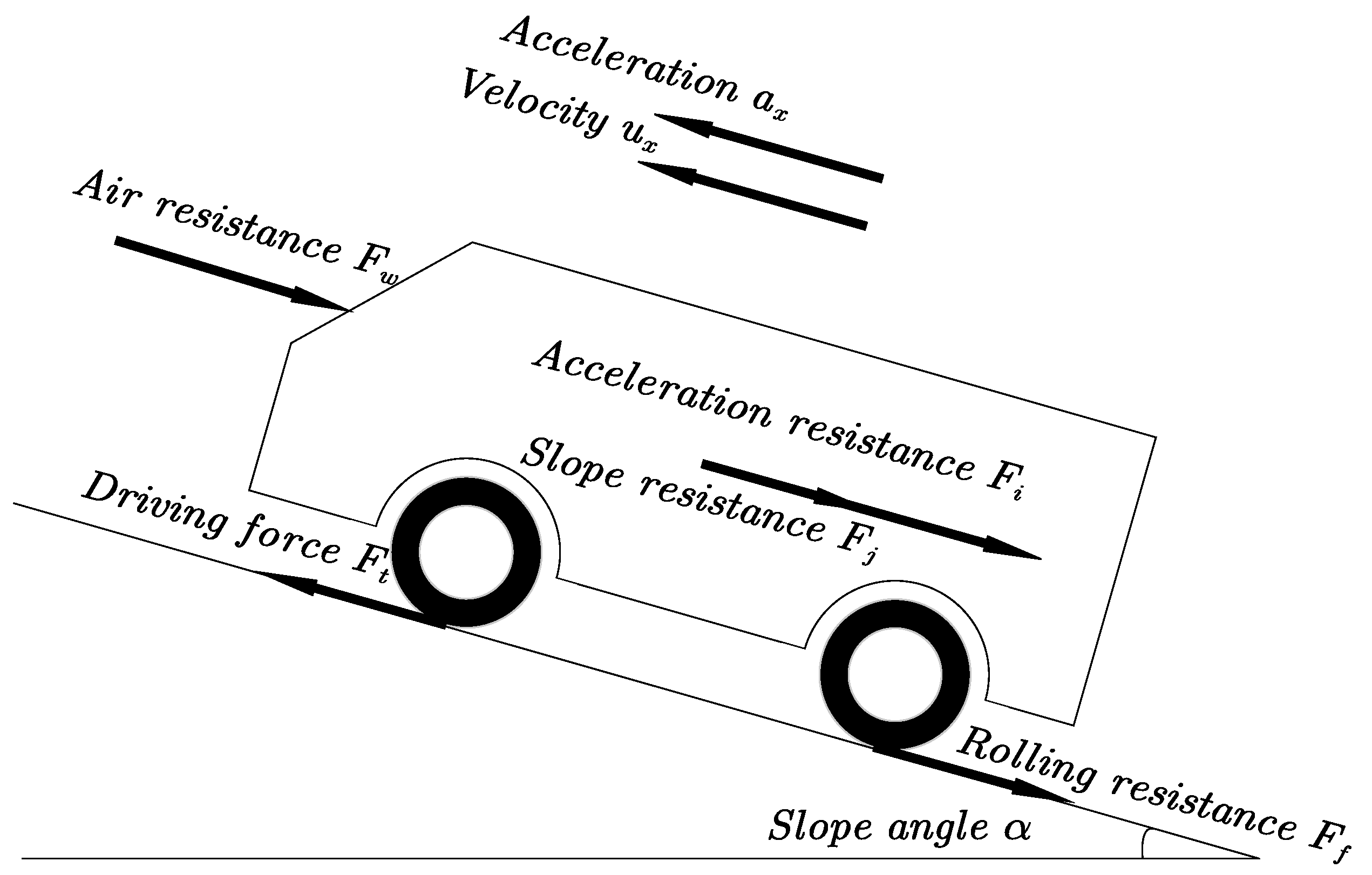
With the help of the transmission system, automobile driving torque T t q can finally go to the driving wheels. The corresponding reaction force of the ground will propel the vehicle move forward. The various forces on the vehicle during the uphill process are as shown in Figure 3. Considering only the longitudinal dynamics, the model of the vehicle can be developed as follows:
F t = F f + F w + F j + F i
where F t , F f , F w , F j , and F i refer to the driving force, rolling resistance, air resistance, acceleration resistance and slope resistance, respectively.
The driving force F t can be expressed as:
F t = T t q i g i 0 η T r
where i g is the gear ratio of the transmission, i 0 is the gear ratio of the final drive, η T is the transmission mechanical efficiency, r is the effective radius of rotating tire, respectively.
The acceleration resistance F j is defined as:
F j = δ m a x
where δ is the rotating mass conversion factor, m is the total vehicle mass, a x is the vehicle longitudinal acceleration, respectively.
The air resistance F w when there is no wind is as follows:
F w = 1 2 ρ C d A f u x 2
where ρ is the air density, C d is the aerodynamic drag coefficient, A f is the frontal area of the vehicle, u x is the vehicle longitudinal speed, respectively.
The rolling resistance F f is defined as:
F f = m g f cos α
where g is the acceleration of gravity, f is the coefficient of rolling resistance, and α is the angle of slope, respectively.
The slope resistance F i is defined as:
F i = m g sin α
Integrate formulas of each force into (6) yields:
T t q i g i 0 η T r = δ m a x + 1 2 ρ C d A f u x 2 + m g f cos α + m g sin α
Given that the transmission ratio is not always available in advance and that the effective tire radius varies and is challenging to determine, the transmission to wheel ratio is approximated here using the vehicle’s speed and engine speed:
i r = i g i 0 r = π 30 n u x
where i r is defined as the ratio of i g i 0 to r .
Therefore, (12) is transformed into:
δ m a x = π 30 T t q η T n u x 1 2 ρ C d A f u x 2 m g ( f cos α + sin α )
As seen in (14), at the very least, driving force, longitudinal acceleration, longitudinal velocity, and slope angle should be gathered in order to determine vehicle mass. They can be collected using sensors, such as IMU and GNSS, which are frequently used in autonomous vehicles.
The neural network input feature vector is expressed as follows:
A i n p u t = F t F w δ a x ( f cos α + sin α ) g v x T
where v x is velocity expressed in km/h.
The transmission of information in a classic feedforward neural network is unidirectional, with the current input being transmitted forward layer by layer through the neural network, corresponding to the current output. In real tasks, however, the output of the current time is influenced not just by the current time input, but also by the historical time. As a result, the back step of A i n p u t is taken into account and supplied into the neural network.

2.2.3. Neural Network Architecture

For multi-head attention, 16 parallel attention heads are adopted. The amount of dropout applied to all linear layers is 0.3. The encoder block applied consists of 3 encoder layers.

2.3. Confidence Level for Weight Adjustment

The weight between EKF and the transformer neural network estimation results is represented by the weight factor, which impacts their weight in the final estimation results. The confidence level is calculated by comparing the training and test datasets for similarity. A subspace partition of training data and mapping of test data is presented in [28]. However, it necessitates a significant amount of computing. A new approach is being developed here. Assume the variable x = F t a x v x α T in the training dataset’s state quantity vector x follows the multivariate normal distribution:
p ( x ; μ , Σ ) = 1 ( 2 π ) n 2 | Σ | 1 2 exp 1 2 ( x μ ) T Σ 1 ( x μ )
where μ is the mean vector, Σ is the covariance vector, n represents the number of features of x, and | Σ | det Σ is the determinant of Σ . Therefore, the probability density at μ of the training data is:
p m a x = 1 ( 2 π ) n 2 | Σ | 1 2
During the application of estimation, every time a new datapoint is fed into the neural network, substitute its value into (16), and get the corresponding probability density:
p k = 1 ( 2 π ) n 2 | Σ | 1 2 exp 1 2 ( x k μ ) T Σ 1 ( x k μ )
Here, the probability density of the test dataset point will be divided by the maximum probability density in the training dataset, i.e., p m a x to get the final confidence level:
τ k = p k p m a x = exp 1 2 ( x k μ ) T Σ 1 ( x k μ )

2.4. AEKF

In comparison to RLS, KF is a correction-based recursive algorithm. It realizes the parameter estimation of a linear system with the minimum variance criterion. KF and its variants are frequently adopted for state estimation in linear systems [35,36]. For systems with non-linear transition equations or measurement equations, EKF is derived to linearize the equations. Different Kalman filter extensions (e.g., UKF, cubature KF (CKF)) have been adopted in various fields [37,38,39]. However, EKF performs better in terms of real-time performance, computing efficiency and parameter tuning in engineering applications. It is assumed that the nonlinear system has the following nonlinear state transition equation and observation equation:
x k = g ( x k 1 , μ k 1 ) + w k 1
y k = h ( x k ) + v k
where x k is the state quantity at step k, y k is the observation quantity, μ is the control quantity, g is the transition function, h is the observation function, w is process noise, subject to N 0 , Q w , v is observation noise, subject to N 0 , R v .
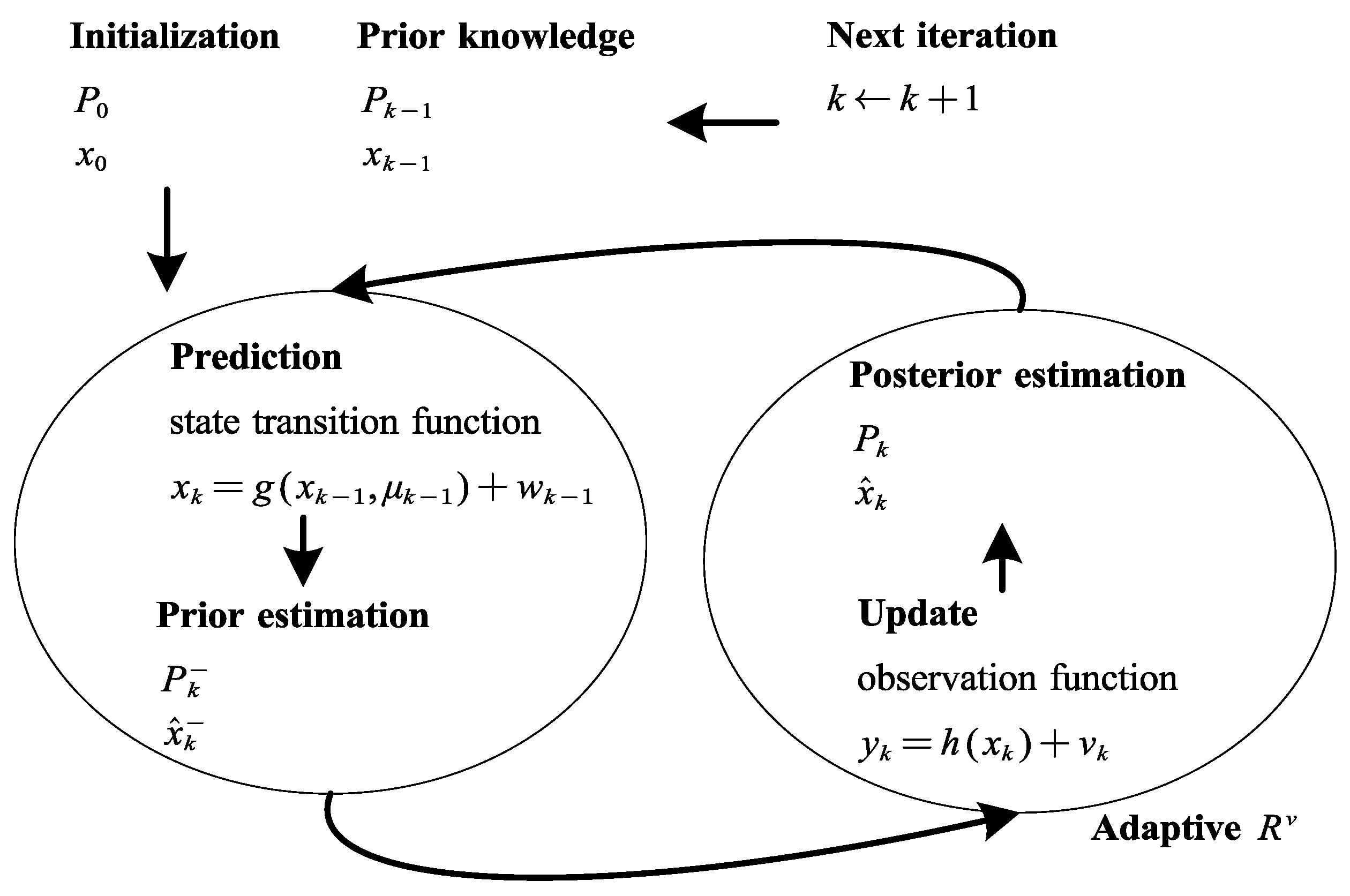
The procedure of EKF is a series of successive operations of prediction based on state input and update based on measurement output.
First, the prior state estimation of state quantity x ^ k is calculated by:
x ^ k = g ( x ^ k 1 , μ k 1 )
and then the prior state estimation of covariance matrix P k is calculated by:
P k = A P k 1 A T + Q w
The Kalman gain K k is calculated by:
K k = P k H T ( H P k H T + R v ) 1
Therefore, the posterior state estimation of state quantity x ^ k is corrected with measurements by:
x ^ k = x ^ k + K k ( y k H x ^ k )
and the posterior state estimation of covariance matrix P k is updated by:
P k = I K k H P k
Here, A and H are the Jacobian matrices, calculated by the partial derivative of state transition function g and observation function h to state quantity x, respectively.
A = g x
H = h x
In order to apply EKF, the state space model is established. The longitudinal speed and vehicle mass are selected as the state quantity:
x k = v x 1 m T
The state equation form is derived to be:
v x k 1 m k = g 1 g 2 + w k 1 = v k 1 + a x Δ T 1 m k 1 + w k 1
The observation quantity is chosen as follows:
y k = v x k
The Jacobian matrix is:
A = g 1 v g 1 1 m g 2 v g 2 1 m = A 11 A 12 0 1
where
A 11 = 1 3.6 Δ T δ m 3 π 25 T t q η T n v 2 + 1 12.96 ρ C D A v x
A 12 = 3.6 Δ T δ 3 π 25 T t q η T n v 1 25.92 ρ C D A v x 2
The new observation quantity is chosen by expanding the original observation y k with the transformer pre-estimation y n n k as follows:
y ˜ k = y k y n n k
y n n k = 1 m n n k
where m n n k will be the estimated mass value of neural network.
Based on the weight adjustment module, an adaptive law is utilized to integrate the pre-estimation of the transformer into the AEKF. The flow chart of AEKF is shown in Figure 4. The pseudocode of TA-AEKF is shown in Algorithm 1, where R n n v = σ m n n 2 represents the observation covariance matrix increased by the neural network. Instead of using τ k and ( 1 τ k ) as the weight factor, here divide them by τ k and use ( τ k ) / τ k = 1 and ( 1 τ k ) / τ k to adjust the observation covariance matrix of neural network.
Algorithm 1 Transformer Aided Adaptive Extended Kalman Filter
  • function Deep Adaptive EKF
  • x ^ 0 Initialization
  • P 0 Initialization
  • for k 1 to N do
  •     x ^ k g ( x ^ k 1 , μ k 1 )
  •     Q ˜ k w Q k w
  •     P k A P k 1 A T + Q ˜ k w
  •     R ˜ k v R v 0 0 1 τ k / τ k R n n v
  •     K k P k H T ( H P k H T + R ˜ k v ) 1
  •     y ˜ k y k y n n k T
  •     x ^ k x ^ k + K k y ˜ k H x ^ k
  •     P k I K k H P k
  • end for
  • return x ^ N , P N
  • end function
As τ ( 0 , 1 ] , therefore ( 1 τ k ) / τ k [ 0 , + ) . In case when the new input data of the neural network is far from the original dataset, τ approaches zero. ( 1 τ k ) / τ k approaches + . The posterior state x ^ k relies more on the matching degree between the physical model and the actual driving condition. As the similarity grows, the value τ increases gradually. If τ equals one, the observation covariance part based on the neural network equals zero. The final estimation result is completely based on a neural network.

3. Data Acquisition

For a data-driven approach such as the transformer, the amount and richness of the data may directly affect how the network functions. The dataset must include an adequate amount of data samples and should resemble actual ones. The neural network is tested using simulation data produced by the high-fidelity Truck-Sim model.
By configuring the settings for the truck model and the testing environment in TruckSim, gather sensor data in the virtual environment, and assess the accuracy of the parameter estimate technique. The main parameters of simulation vehilc e is shown in Table 1. The simulated vehicle’s curb weight is 6042 kg. A range of payloads is selected, ranging from 4000 to 40,000 kg every 4000 kg.
Different slope conditions are used to generate enough simulation data. Five kinds of slope conditions are shown in Figure 5a, and the highway fuel economy driving schedule (HWFET) speed profile condition shown in Figure 5b are adopted. Each payload value and slope condition is combined to collect enough information. Each simulation is 100 s long.
In order to verify the accuracy and stability of the proposed method, two simulation tests are conducted. The gross vehicle weight is set to be 28,542 kg. The other parameters remain the same as the vehicle used for simulation data collection. Two kinds of slope conditions are used for test data generation, shown in Figure 6.

4. Results

The proportion of the training set, test set, and validation set are 6:2:2. The training of the neural network is implemented in Pytorch and Tsai [40]. The experiments were conducted on Ubuntu 20.04 operating system computer, which is equipped with Intel(R) Core(TM) i5-10600 CPU @ 3.30 GHz CPU, 64 G RAM and 12GB GeForce RTX 3080.

4.1. Evaluation Metrics

The root mean square error (RMSE), mean absolute error (MAE), and mean absolute percentage error (MAPE) are used as evaluation metrics to assess the accuracy of mass estimate results:
RMSE = 1 n i = 1 n m i ^ m 2
MAE = 1 n i = 1 n m ^ i m
MAPE = 100 % n i = 1 n m ^ i m m
where m i ^ is the estimated value of mass, m is the ground truth of mass, n is the total number of estimated mass values.
In order to evaluate the stability of estimation results, here the convergence rate (CR) is adopted to evaluate the stability of estimation [41]. The estimation result is deemed to be convergent when the following requirements are satisfied:
c v ( m ^ ) = σ ( m ^ ) μ ( m ^ ) < c v 0
m ^ i m m < 2 %
where c v is the coefficient of variation, defined as the standard variance of estimation σ ( m ^ ) divided by the mean of estimation μ ( m ^ ) , and c v 0 is the threshold of c v and set to be 0.02. CR is defined as the calculation steps cost when c v converges to lower than c v 0 .

4.2. Performance Evaluation

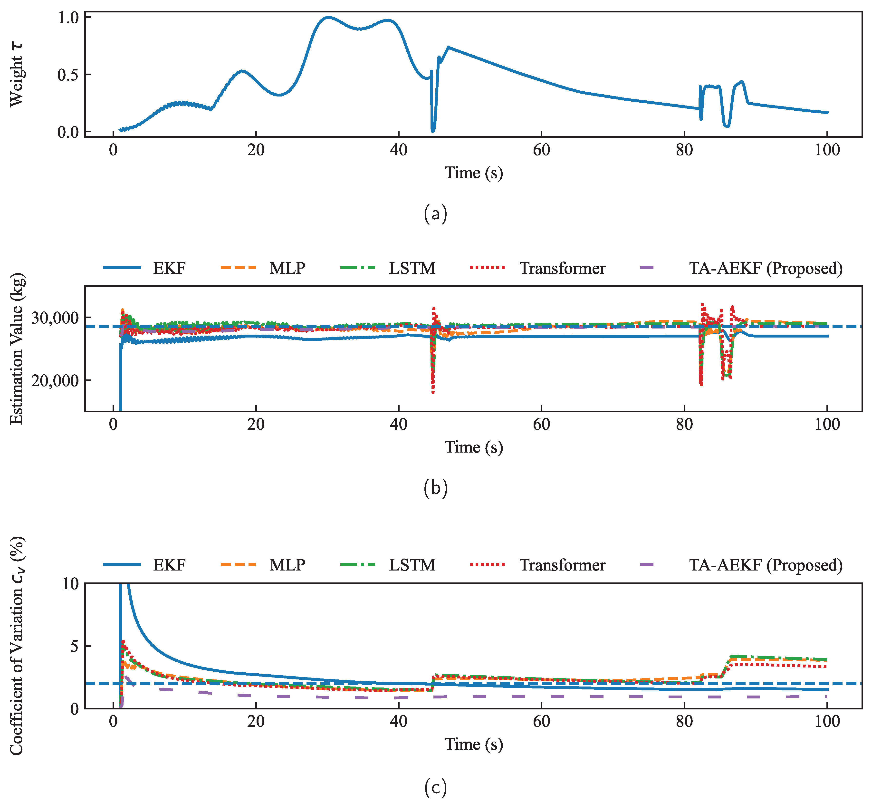
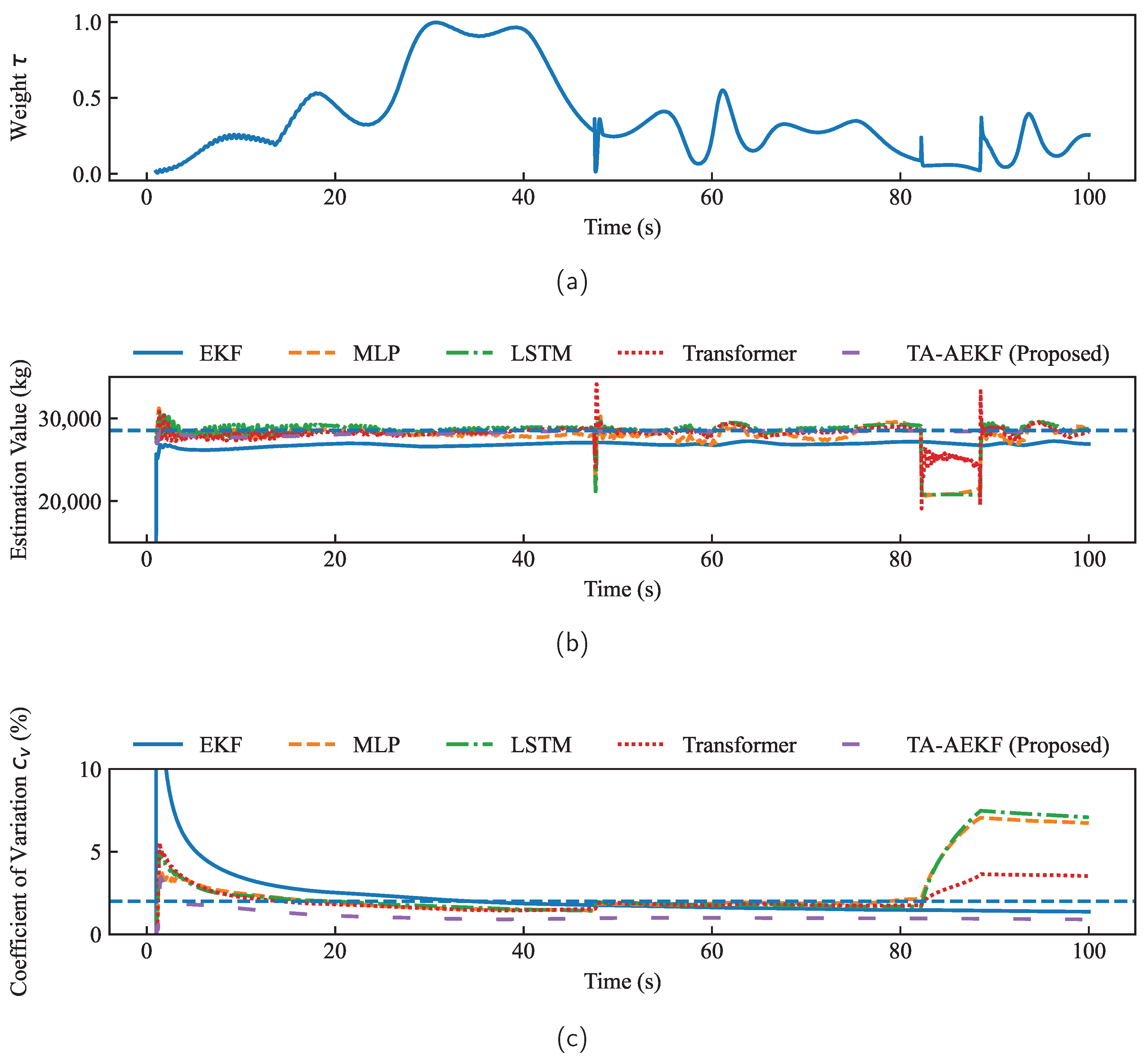
The estimation results of each test are shown in Figure 7 and Figure 8. The blue dashed line represents the result of ground truth in the middle subgraph and c v 0 = 2 % in the bottom subgraph, respectively.
In Figure 7a, the weight level of test 1 changes due to the difference between the training set and the test set. Shown in Figure 7b, the estimation results of the neural network estimator vary and fluctuate occasionally. The transformer shows higher oscillations, followed by LSTM and MLP. However, these oscillations are not allowed in the control system as they would break the stability of the system. On the other hand, the estimation result of EKF is more stable. To start with, the EKF result undershoots to some high value but then begins to converge to ground truth gradually, showing more stability. The estimation results of the proposed method neither overshoot nor oscillates. Figure 7c shows the coefficient of variation and demonstrates the stability of each method. c v of neural network methods gradually rises and is higher than 2 % in the end, while the result of EKF overshoots and converges to lower than 2 % . The result of the proposed method rises like neural network estimators, but will finally converge to a stable value lower than 2 % .
In Figure 8a, the weight level of Test 2 changes more frequently, and the results of neural network estimators will also oscillate, which also shows the instability of neural network results, and might do harm to control systems. The changing trend of results also shows the advantages of the proposed method.
The metrics listed in Table 2, Table 3 and Table 4 demonstrate the superiority of the proposed method in terms of accuracy, with lower values in MAPE, RMSE, and MAE. RMSE and MAE are used to measure the deviation between the ground truth value and the predicted value, whereas MAPE measures the relative size of the deviation. RMSE and MAE have the same dimensions as the quantity, while MAPE is dimensionless. RMSE is more sensitive to outliers and can magnify prediction errors due to the square operation. In contrast, MAE and MAPE are more robust to extreme values.
In test 1, the MAE of LSTM is smaller than that of MLP, but LSTM has a higher value of RMSE, indicating that there are higher extreme values in LSTM’s estimation. As for test 2, EKF has the highest value of MAE, indicating the maximum number of estimation errors. However, LSTM and MLP have higher values of RMSE, indicating higher deviations in the results of neural network estimators. MAPE is easier to understand, even when the ground truth values are different, whereas MAE and RMSE need to combine the real value to judge the difference. These discrepancies are also apparent from Figure 7 and Figure 8.
In terms of the time needed to converge to the threshold of efficiency variation, the proposed method is faster, demonstrating its stability advantage. Furthermore, among the three neural network estimators, the transformer neural network demonstrates superior performance. However, it should be noted that all neural network estimators exhibit instability, as they are unable to converge below the threshold of 2%. These further prove the necessity of integrating EKF with the transformer.

4.3. Input Feature Demonstration

To prove that the input feature is selected for the neural network, here the permutation method is used. In addition to the original features, lateral acceleration a y and yaw rate ω are also fed into the neural network. The MAPE increase when a feature is removed is calculated, shown in Figure 9. The removal of features included in A t would result in higher MAPE than a y and ω . Therefore, just selecting the input features in A t is enough to recharacterize the nonlinear dynamics.

4.4. Confidence Level Demonstration

4.4.1. Calculation Speed Demonstration

To better demonstrate the calculation speed of the confidence level module, the computing time of each method is calculated as shown in Table 5. Results prove the outperformance of the proposed method in terms of calculation speed of confidence level.

4.4.2. Improtance Demonstration

To better demonstrate the importance of the weight adjustment module, here different values are chosen to balance the relationship between the transformer and AEKF. The weight factor is set to be 10 15 , 1 and the adaptive weight τ x , respectively. Furthermore, the results are shown in Figure 10 and Table 6. When τ equals one, ( 1 τ k ) / τ k equals zero. In this case, the result of TA-AEKF is the same as the estimation of the transformer. lim x 0 is represented by setting τ = 10 15 . Furthermore, the result would be more reliant on the dynamic model. TA-AEKF estimator results when τ = τ k has the lowest MAPE, MAE, and RMSE. As for convergence steps, the values of τ = 10 15 and τ = τ k are very close. Therefore, the adaptive τ = τ x does work.

4.5. Real Time Test

To better evaluate the real-time performance of the proposed method, the corresponding computing time is calculated. For neural network estimators, the model can be trained offline and loaded before estimation. As shown in Table 7, LSTM costs the lowest time and TA-AEKF costs the highest. Besides, for a certain driving process, the total mass remains constant. Therefore, the calculation of mass can be done just once by collecting enough data. In this case, the computing time of the proposed method meets the need for the requested real-time performance.

5. Conclusions

In order to further improve the accuracy and robustness of autonomous vehicle mass estimation, the transformer-aided adaptive extended Kalman filter is proposed by integrating the transformer pre-estimation into an extended Kalman filter using a weight adjustment module. Simulation tests are conducted to validate the appropriateness of neural network feature selection, the adaptive law of the proposed weight adjustment module and the accuracy and stability of the proposed method.
In future work, we extend to collect more real vehicle data under more complex working conditions for performance verification. Furthermore, the proposed method will be extended to the estimation of other parameters in autonomous vehicles and different fields.

Author Contributions

Conceptualization, H.X. and Z.Y.; methodology, H.Z. and Z.Y.; investigation, Z.Y. and T.Z.; writing—original draft preparation, Z.Y.; writing—review and editing, H.Z., H.X., T.Z., Z.L. and W.W.; supervision, H.X.; funding acquisition, H.X. All authors have read and agreed to the published version of the manuscript.

Funding

This research is funded by the Key-Area Research and Development Program of Guangdong Province (2020B0909050004) and Natural Science and Technology Special Projects under Grant 2019-1496.

Institutional Review Board Statement

Not applicable.

Informed Consent Statement

Not applicable.

Data Availability Statement

Data sharing not applicable.

Conflicts of Interest

The authors declare no conflict of interest.

References

  1. Singh, K.B.; Arat, M.A.; Taheri, S. Literature Review and Fundamental Approaches for Vehicle and Tire State Estimation. Veh. Syst. Dyn. 2019, 57, 1643–1665. [Google Scholar] [CrossRef]
  2. Xiong, H.; Tan, Z.; Zhang, R.; He, S. A New Dual Axle Drive Optimization Control Strategy for Electric Vehicles Using Vehicle-to-Infrastructure Communications. IEEE Trans. Ind. Inform. 2020, 16, 2574–2582. [Google Scholar] [CrossRef]
  3. Xiong, H.; Zhu, X.; Zhang, R. Energy Recovery Strategy Numerical Simulation for Dual Axle Drive Pure Electric Vehicle Based on Motor Loss Model and Big Data Calculation. Complexity 2018, 2018, e4071743. [Google Scholar] [CrossRef] [Green Version]
  4. Liu, W.; Xiong, L.; Xia, X.; Lu, Y.; Gao, L.; Song, S. Vision-Aided Intelligent Vehicle Sideslip Angle Estimation Based on a Dynamic Model. IET Intell. Transp. Syst. 2020, 14, 1183–1189. [Google Scholar] [CrossRef]
  5. Xia, X.; Hashemi, E.; Xiong, L.; Khajepour, A. Autonomous Vehicle Kinematics and Dynamics Synthesis for Sideslip Angle Estimation Based on Consensus Kalman Filter. IEEE Trans. Control. Syst. Technol. 2023, 31, 179–192. [Google Scholar] [CrossRef]
  6. Yang, S.K.; Liu, T.S.; Cheng, Y.C. Automatic Measurement of Payload for Heavy Vehicles Using Strain Gages. Measurement 2008, 41, 491–502. [Google Scholar] [CrossRef]
  7. AG, C. Continental In-Tire Sensors Read Tread Depth. 2014. Available online: https://www.continental.com/en/press/press-releases/2014-05-07-tpms-profile-104542 (accessed on 14 April 2021).
  8. Zhang, Y.; Zhang, Y.; Ai, Z.; Feng, Y.; Zhang, J.; Murphey, Y.L. Estimation of Electric Mining Haul Trucks’ Mass and Road Slope Using Dual Level Reinforcement Estimator. IEEE Trans. Veh. Technol. 2019, 68, 10627–10638. [Google Scholar] [CrossRef]
  9. Torabi, S.; Wahde, M.; Hartono, P. Road Grade and Vehicle Mass Estimation for Heavy-duty Vehicles Using Feedforward Neural Networks. In Proceedings of the 2019 4th International Conference on Intelligent Transportation Engineering (ICITE), Singapore, 5–7 September 2019; IEEE: Singapore, 2019; pp. 316–321. [Google Scholar] [CrossRef]
  10. Wang, H.; Zheng, Y.; Yu, Y. Joint Estimation of SOC of Lithium Battery Based on Dual Kalman Filter. Processes 2021, 9, 1412. [Google Scholar] [CrossRef]
  11. Feng, W.; Dong, W.; Zhai, S.; Zhang, G.; Sun, X.; Ji, Y. A Deep Reinforcement Learning Method for Freight Train Driving Based on Domain Knowledge and Mass Estimation Network. In Proceedings of the 2021 6th International Conference on Machine Learning Technologies, Jeju Island, Republic of Korea, 23–25 April 2021; ACM: New York, NY, USA, 2021; pp. 41–46. [Google Scholar] [CrossRef]
  12. Ritter, A.; Widmer, F.; Vetterli, B.; Onder, C.H. Optimization-Based Online Estimation of Vehicle Mass and Road Grade: Theoretical Analysis and Experimental Validation. Mechatronics 2021, 80, 102663. [Google Scholar] [CrossRef]
  13. Li, X.; Ma, J.; Zhao, X.; Wang, L. Intelligent Two-Step Estimation Approach for Vehicle Mass and Road Grade. IEEE Access 2020, 8, 218853–218862. [Google Scholar] [CrossRef]
  14. Zhang, F.; Wang, Y.; Hu, J.; Yin, G.; Chen, S.; Zhang, H.; Zhou, D. A Novel Comprehensive Scheme for Vehicle State Estimation Using Dual Extended H-Infinity Kalman Filter. Electronics 2021, 10, 1526. [Google Scholar] [CrossRef]
  15. Mei, C.; Peng, J.; Yuhui, H. An Online Mass Estimation Algorithm for Single-shaft Parallel Hybrid Commercial Vehicle. Acta Armamentarii 2021, 42, 1838–1846. [Google Scholar] [CrossRef]
  16. Zhang, Z.; Yin, G.; Wu, Z. Joint Estimation of Mass and Center of Gravity Position for Distributed Drive Electric Vehicles Using Dual Robust Embedded Cubature Kalman Filter. Sensors 2022, 22, 10018. [Google Scholar] [CrossRef]
  17. Rajamani, R.; Hedrick, J.K. Adaptive Observers for Active Automotive Suspensions: Theory and Experiment. IEEE Trans. Control. Syst. Technol. 1995, 3, 86–93. [Google Scholar] [CrossRef]
  18. Jensen, K.M.; Santos, I.F.; Clemmensen, L.K.H.; Theodorsen, S.; Corstens, H.J.P. Mass Estimation of Ground Vehicles Based on Longitudinal Dynamics Using IMU and Can-Bus Data. Mech. Syst. Signal Process. 2022, 162, 107982. [Google Scholar] [CrossRef]
  19. Reina, G.; Paiano, M.; Blanco-Claraco, J.L. Vehicle Parameter Estimation Using a Model-Based Estimator. Mech. Syst. Signal Process. 2017, 87, 227–241. [Google Scholar] [CrossRef] [Green Version]
  20. Jeong, D.; Kim, S.; Lee, J.; Choi, S.B.; Kim, M.; Lee, H. Estimation of Tire Load and Vehicle Parameters Using Intelligent Tires Combined With Vehicle Dynamics. IEEE Trans. Instrum. Meas. 2020, 70, 1–12. [Google Scholar] [CrossRef]
  21. Cai, L.; Wang, H.; Jia, T.; Peng, P.; Pi, D.; Wang, E. Two-Layer Structure Algorithm for Estimation of Commercial Vehicle Mass. Proc. Inst. Mech. Eng. Part D J. Automob. Eng. 2020, 234, 378–389. [Google Scholar] [CrossRef]
  22. Jin, X.; Yang, J.; Li, Y.; Zhu, B.; Wang, J.; Yin, G. Online Estimation of Inertial Parameter for Lightweight Electric Vehicle Using Dual Unscented Kalman Filter Approach. IET Intell. Transp. Syst. 2020, 14, 412–422. [Google Scholar] [CrossRef]
  23. Sun, S.; Zhang, N.; Walker, P.; Lin, C. Intelligent Estimation for Electric Vehicle Mass with Unknown Uncertainties Based on Particle Filter. IET Intell. Transp. Syst. 2020, 14, 463–467. [Google Scholar] [CrossRef]
  24. Chen, J.; Feng, X.; Jiang, L.; Zhu, Q. State of Charge Estimation of Lithium-Ion Battery Using Denoising Autoencoder and Gated Recurrent Unit Recurrent Neural Network. Energy 2021, 227, 120451. [Google Scholar] [CrossRef]
  25. Barati, K.; Shen, X.; Li, N.; Carmichael, D.G. Automatic Mass Estimation of Construction Vehicles by Modeling Operational and Engine Data. J. Constr. Eng. Manag. 2022, 148, 04021208. [Google Scholar] [CrossRef]
  26. Xiong, H.; Wang, Z.; Wu, G.; Pan, Y.; Yang, Z.; Long, Z. Steering Actuator Fault Diagnosis for Autonomous Vehicle With an Adaptive Denoising Residual Network. IEEE Trans. Instrum. Meas. 2022, 71, 1–13. [Google Scholar] [CrossRef]
  27. Korayem, A.H.; Khajepour, A.; Fidan, B. Trailer Mass Estimation Using System Model-Based and Machine Learning Approaches. IEEE Trans. Veh. Technol. 2020, 69, 12536–12546. [Google Scholar] [CrossRef]
  28. Sieberg, P.M.; Blume, S.; Reicherts, S.; Maas, N.; Schramm, D. Hybrid State Estimation-A Contribution Towards Reliability Enhancement of Artificial Neural Network Estimators. IEEE Trans. Intell. Transp. Syst. 2022, 23, 6337–6346. [Google Scholar] [CrossRef]
  29. Hannan, M.A.; How, D.N.T.; Lipu, M.S.H.; Mansor, M.; Ker, P.J.; Dong, Z.Y.; Sahari, K.S.M.; Tiong, S.K.; Muttaqi, K.M.; Mahlia, T.M.I.; et al. Deep Learning Approach towards Accurate State of Charge Estimation for Lithium-Ion Batteries Using Self-Supervised Transformer Model. Sci. Rep. 2021, 11, 19541. [Google Scholar] [CrossRef]
  30. Pang, H.; Liu, F.; Xu, Z. Variable Universe Fuzzy Control for Vehicle Semi-Active Suspension System with MR Damper Combining Fuzzy Neural Network and Particle Swarm Optimization. Neurocomputing 2018, 306, 130–140. [Google Scholar] [CrossRef]
  31. Xing, Y.; Lv, C. Dynamic State Estimation for the Advanced Brake System of Electric Vehicles by Using Deep Recurrent Neural Networks. IEEE Trans. Ind. Electron. 2020, 67, 9536–9547. [Google Scholar] [CrossRef]
  32. Lin, C.; Wang, H.; Fu, M.; Yuan, J.; Gu, J. A Gated Recurrent Unit-Based Particle Filter for Unmanned Underwater Vehicle State Estimation. IEEE Trans. Instrum. Meas. 2020, 70, 1–12. [Google Scholar] [CrossRef]
  33. Wang, M.; Pang, H.; Luo, J.; Liu, M. On an Enhanced Back Propagation Neural Network Control of Vehicle Semi-Active Suspension with a Magnetorheological Damper. Trans. Inst. Meas. Control. 2023, 45, 512–523. [Google Scholar] [CrossRef]
  34. Zerveas, G.; Jayaraman, S.; Patel, D.; Bhamidipaty, A.; Eickhoff, C. A Transformer-Based Framework for Multivariate Time Series Representation Learning. In Proceedings of the 27th ACM SIGKDD Conference on Knowledge Discovery & Data Mining, Singapore, 14–18 August 2021; ACM: New York, NY, USA, 2021; pp. 2114–2124. [Google Scholar] [CrossRef]
  35. Hong, S.; Lee, C.; Borrelli, F.; Hedrick, J.K. A Novel Approach for Vehicle Inertial Parameter Identification Using a Dual Kalman Filter. IEEE Trans. Intell. Transp. Syst. 2015, 16, 151–161. [Google Scholar] [CrossRef]
  36. Xiong, L.; Xia, X.; Lu, Y.; Liu, W.; Gao, L.; Song, S.; Yu, Z. IMU-Based Automated Vehicle Body Sideslip Angle and Attitude Estimation Aided by GNSS Using Parallel Adaptive Kalman Filters. IEEE Trans. Veh. Technol. 2020, 69, 10668–10680. [Google Scholar] [CrossRef]
  37. Xiong, H.; Liu, J.; Zhang, R.; Zhu, X.; Liu, H. An Accurate Vehicle and Road Condition Estimation Algorithm for Vehicle Networking Applications. IEEE Access 2019, 7, 17705–17715. [Google Scholar] [CrossRef]
  38. Yang, F.; Zhang, S.; Li, W.; Miao, Q. State-of-Charge Estimation of Lithium-Ion Batteries Using LSTM and UKF. Energy 2020, 201, 117664. [Google Scholar] [CrossRef]
  39. Liu, W.; Xia, X.; Xiong, L.; Lu, Y.; Gao, L.; Yu, Z. Automated Vehicle Sideslip Angle Estimation Considering Signal Measurement Characteristic. IEEE Sens. J. 2021, 21, 21675–21687. [Google Scholar] [CrossRef]
  40. Oguiza, I. tsai - A State-of-the-Art Deep Learning Library for Time Series and Sequential Data; Github: San Francisco, CA, USA, 2022. [Google Scholar]
  41. Kidambi, N.; Harne, R.L.; Fujii, Y.; Pietron, G.M.; Wang, K.W. Methods in Vehicle Mass and Road Grade Estimation. SAE Int. J. Passeng. Cars-Mech. Syst. 2014, 7, 981–991. [Google Scholar] [CrossRef] [Green Version]
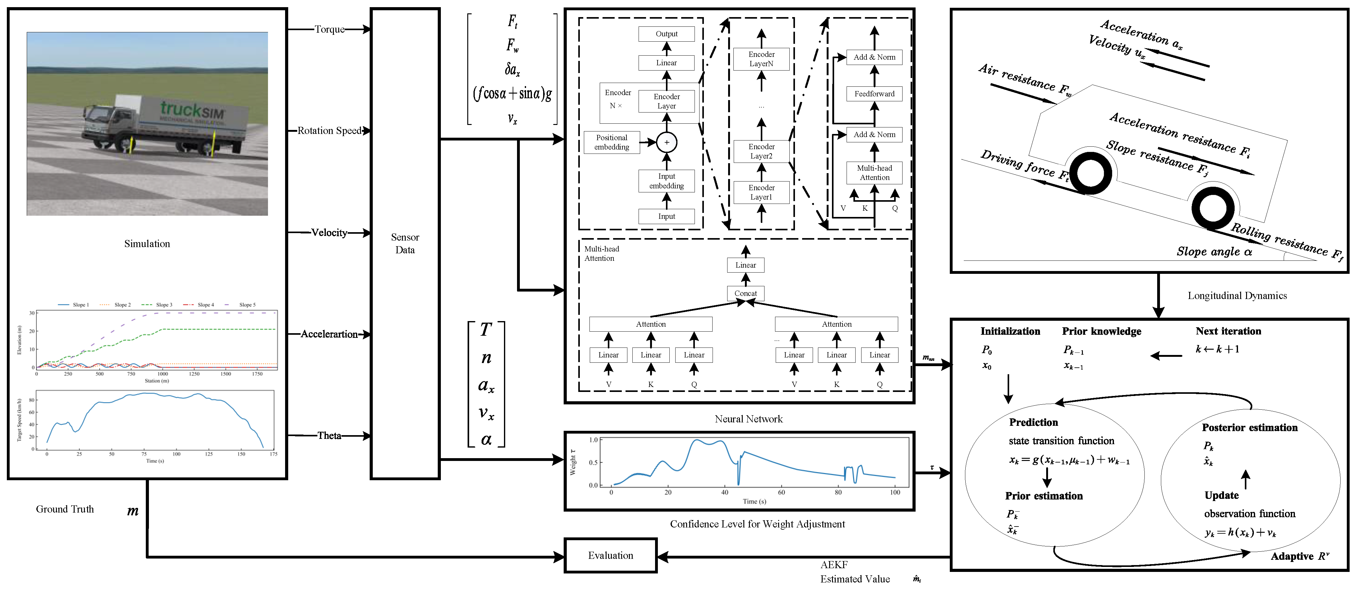
Figure 1. The framework of the proposed TA-AEKF estimator.
Processes 11 00887 g001
Figure 2. The flow chart of the proposed transformer model.
Processes 11 00887 g002
Figure 3. The force analysis of a vehicle moving on a slope.
Processes 11 00887 g003
Figure 4. The architecture of AEKF.
Processes 11 00887 g004
Figure 5. Simulation conditions: (a) Slopes profiles. (b) Speed profiles.
Processes 11 00887 g005
Figure 6. Slopes of simulation test conditions.
Processes 11 00887 g006
Figure 7. Simulation result of test 1: (a) Weight calculation. (b) Estimation value of mass. The blue dashed line represents the result of the ground truth. (c) Evaluation with c v . The blue dashed line represents c v 0 = 2 % .
Processes 11 00887 g007
Figure 8. Simulation result of test 2: (a) Weight calculation. (b) Estimation value of mass. The blue dashed line represents the result of ground truth. (c) Evaluation with c v . The blue dashed line represents c v 0 = 2 % .
Processes 11 00887 g008
Figure 9. Permutation feature importance shown by MAPE increases when the corresponding feature is removed.
Processes 11 00887 g009
Figure 10. Simulation result of test 1 data using different values of weight to adjust: (a) Estimation value of mass. The blue dashed line represents the result of ground truth. (b) Evaluation with c v . The blue dashed line represents c v 0 = 2 % .
Processes 11 00887 g010
Table 1. Main parameters of simulation vehicle.
ParameterValue
vehicle curb weight6042 kg
vehicle payload4000 to 40,000 per 4000 kg
Frontal area6.8 m 2
efficiency0.99
sample time0.01 s
Table 2. Evaluation metrics of simulation test 1 results.
MethodMAPE
(%)
MAE
(kg)
RMSE
(kg)
CR
(steps)
EKF5.851669.771719.583790
MLP2.28652.051117.12nan
LSTM1.80514.511124.30nan
Transformer1.42404.91972.35nan
TA-AEKF
(Proposed)
0.89255.41356.42156
Table 3. Evaluation metrics of simulation test 2 results.
MethodMAPE
(%)
MAE
(kg)
RMSE
(kg)
CR
(steps)
EKF5.981706.401745.783338
MLP3.571018.142031.73nan
LSTM2.95843.072018.19nan
Transformer2.15613.111068.24nan
TA-AEKF
(Proposed)
0.90257.53357.61212
Table 4. Evaluation metrics of simulation test 1 & 2 average results.
MethodMAPE
(%)
MAE
(kg)
RMSE
(kg)
CR
(steps)
EKF5.911688.081732.683564
MLP2.93835.091574.42nan
LSTM2.38678.791571.25nan
Transformer1.78509.011020.29nan
TA-AEKF
(Proposed)
0.90256.47357.01184
Table 5. Evaluation computing time of weight adjustment.
MethodComputing Time (s)
Test1Test2Average of Test1 & Test2
Method 1 ([28])280.21293.68286.94
Method 2 (Proposed)1.000.991.00
Table 6. Evaluation metrics of different weight factors.
MethodMAPE
(%)
MAE
(kg)
RMSE
(kg)
CR
(steps)
τ = 1 e 15 8.062301.152305.04154
τ = 1 1.42404.91972.35nan
τ = τ k 0.89255.41356.42156
Table 7. Evaluation computing time of simulation test.
MethodComputing Time (s)
Test1Test2Average of Test1 & Test2
EKF0.530.570.55
MLP0.170.210.19
LSTM0.170.180.17
Transformer0.440.460.45
TA-AEKF (Proposed)1.071.091.08
Disclaimer/Publisher’s Note: The statements, opinions and data contained in all publications are solely those of the individual author(s) and contributor(s) and not of MDPI and/or the editor(s). MDPI and/or the editor(s) disclaim responsibility for any injury to people or property resulting from any ideas, methods, instructions or products referred to in the content.