Article

Achieving Optimal Paper Properties: A Layered Multiscale kMC and LSTM-ANN-Based Control Approach for Kraft Pulping

1
Artie McFerrin Department of Chemical Engineering, Texas A&M University, College Station, TX 77843, USA
2
Texas A&M Energy Institute, Texas A&M University, College Station, TX 77845, USA
*
Author to whom correspondence should be addressed.
Processes 2023, 11(3), 809; https://doi.org/10.3390/pr11030809
Submission received: 28 January 2023 / Revised: 21 February 2023 / Accepted: 24 February 2023 / Published: 8 March 2023
(This article belongs to the Special Issue Machine Learning in Model Predictive Control and Optimal Control)

Abstract

:
The growing demand for various types of paper highlights the importance of optimizing the kraft pulping process to achieve desired paper properties. This work proposes a novel multiscale model to optimize the kraft pulping process and obtain desired paper properties. The model combines mass and energy balance equations with a layered kinetic Monte Carlo (kMC) algorithm to predict the degradation of wood chips, the depolymerization of cellulose, and the spatio-temporal evolution of the Kappa number and cellulose degree of polymerization ( D P ). A surrogate LSTM-ANN model is trained on data generated from the multiscale model under different operating conditions, dealing with both time-varying and time-invariant inputs, and an LSTM-ANN-based model predictive controller is designed to achieve desired set-point values of the Kappa number and cellulose D P while considering process constraints. The results show that the LSTM-ANN-based controller is able to drive the process to desired set-point values with the use of a computationally faster surrogate model with high accuracy and low offset.

1. Introduction

The pulp and paper industry (PPI) is undergoing rapid modernization to meet the growing demand for pulp and paper production as shown in Figure 1 [1]. This demand can be attributed to the increase in the use of packaging paper by companies, such as Amazon and Walmart, the growing manufacturing industry in emerging markets, such as Asia and Africa, and the shift towards online shopping by consumers. As a result, the PPI is focusing on using advanced first-principles models and artificial-intelligence techniques to develop digital twins and process-control systems for improved efficiency, reduced waste, and safer operations [2,3,4,5].
Paper is made up of three substances, lignin, hemicellulose, and cellulose, and is typically produced from wood chips. Lignin, the main component of the cell wall, is a highly branched three-dimensional polymer that acts as a glue to hold cellulose microfibrils together [6]. In order to separate lignin from these cellulosic fibers, a process called delignification is used in a large chemical reactor called a pulp digester [6,7]. The Kappa number, a metric that describes the degree of delignification, is used to evaluate the process, where a Kappa number below 100 for cardboard papers and below 60 for kraft and bleachable white papers is favorable [8,9,10].
Despite efforts to manage waste and recycle fibers, the PPI still generates a large amount of waste product, which poses a significant burden on the industry [11]. Based on a report, 17% of the total global waste comes from paper industries, and discarded paper and paperboard make up roughly 26% of solid municipal waste in landfill sites [12,13].
One potential solution is to mitigate fiber degradation through strength modeling. By meeting the specific standards of paper, the amount of waste generated can be significantly reduced. However, achieving the strength requirements and properties of different paper products can be challenging as each product has its own unique strength standard. The tensile strength of paper is an important strength property, and cellulose is responsible for forming crystalline microfibers with excellent tensile strength [14].
The cellulose degree of polymerization ( D P ) is a measure of the cellulose chain length and is the major factor determining the tensile strength of the product as cellulose is the load-bearing element of a pulp fiber [15,16]. Therefore, a good paper product has a high cellulose D P , which represents high strength, and a low Kappa number, which represents a brighter paper. As the final paper product properties, such as strength and yield, are primarily determined by metrics, such as the Kappa number and D P , it is crucial to optimize the pulping process to achieve these specific properties with desired values.
Kraft pulping is the most commonly used chemical pulping process, accounting for 80% of chemical pulp produced in the United States [17]. During kraft pulping, wood chips are exposed to an aqueous solution, which removes both lignin and hemicellulose. Strong alkaline solvents, such as sodium hydroxide (NaOH), are added to the solution to increase the degree of delignification (i.e., to decrease the Kappa number). However, this also results in the breakdown or degradation of cellulose to glucose [18]. To prevent cellulose degradation and obtain the desired paper properties, it is essential to control the operating conditions, such as the batch cooking time, NaOH concentration, and temperature. There have been several approaches in the literature to develop macroscopic and mesoscopic computational models with the extended Purdue model being the most commonly used [19,20,21,22].
However, these models only consider macroscopic equations. They cannot predict important microscopic properties, such as the Kappa number, fiber morphology, D P , and cell-wall thickness (CWT). Recent studies [6,7,23,24] have developed multiscale models using kinetic Monte Carlo (kMC) algorithms [25,26] to describe these microscopic properties and understand fiber-to-fiber heterogeneity. They also designed a model-based controller using reduced-order models and Kalman filters [27,28]. However, these studies did not discuss how reaction conditions affect the cellulose D P . Additionally, there are few studies in the literature on using machine-learning-based predictive controllers for the pulping process to obtain optimal operating conditions and achieve desired paper properties.
To address these limitations, we propose the development of a novel layered multiscale model that combines the kMC algorithm and extended Purdue model equations. This model aims to describe the temporal evolution of important paper properties, such as the Kappa number and cellulose D P . By building on a previously developed multiscale model, which describes the degradation of solid components at the mesoscale, we further modify it to model the depolymerization kinetics at the microscopic level. Specifically, we take into account that the degradation process occurs on a much faster time scale than depolymerization, and thus multiple depolymerization events occur over a single degradation event, thereby, resulting in a layered multiscale model.
Realistic chemical process models, such as the proposed layered multiscale model, can be too complex to be solved in real-time operations. To overcome this challenge, machine learning (ML) and other system-identification methods are employed to learn mathematical models from data and discover patterns without explicit programming [29,30,31,32]. In this work, we construct a surrogate long short-term memory (LSTM)-artificial neural network (ANN) model using input–output data generated from the multiscale model by running it offline under different operating conditions [33,34,35,36].
We select the LSTM-ANN network to handle a combination of time-varying (i.e., temperature) and time-invariant (i.e., cooking time and NaOH concentration) inputs, which are commonly encountered in chemical processes, particularly the pulping process. LSTMs are known for accurately learning temporal dependencies in sequence data, while ANNs are better at extracting information from time-invariant features [37,38,39].
After obtaining an optimal network through hyperparameter tuning and overfitting analysis, the surrogate model is used as an internal evaluator in an LSTM-ANN-based model predictive controller (MPC). This controller is computationally more efficient as it utilizes a well-trained neural network to obtain the optimal input profiles and achieve the desired set-point values for the Kappa number and cellulose D P while considering the process constraints. The performance of the closed-loop controller is demonstrated through a representative case.
The structure of this article is as follows: In Section 2, the mathematical model for the kraft pulping process is presented. In Section 3, the training of the LSTM-ANN model and the design of the controller are discussed. The results of the multiscale model and controller are presented in Section 4. Finally, our conclusions are presented in Section 5.

2. Layered Multiscale kMC Modeling of a Batch Pulp Digester

The multiscale modeling framework is designed to describe the temporal evolution of microscopic properties (such as the Kappa number, cell morphology, pore size distribution, CWT, and cellulose D P ) and macroscopic properties (such as the temperature and concentration profiles). The proposed model is built upon previous multiscale models [7,23] developed for the kraft pulping process, and further modified them to take into account the effect of both the degradation of wood solid components and the depolymerization of cellulose on the tensile strength of paper [14]. This is motivated by the understanding that these properties play a critical role in determining the quality and strength of the final paper product.
The multiscale model comprises three phases: the solid, entrapped-liquor, and free-liquor phases as illustrated in Figure 2 [40]. The free-liquor phase represents the bulk liquor surrounding the chip phase, which comprises both the solid and entrapped-liquor phases. As the components of the solid phase react with those of the entrapped-liquor phase, they dissolve and transform into components of the liquor phase. The extended Purdue model is used to describe macroscopic phenomena, such as energy balance and mass transport, while microscopic properties, such as the Kappa number and cellulose D P , are described by kMC simulations [19,20]. The multiscale model captures the dynamic interaction between these three phases and the resulting changes in properties at both the macroscopic and microscopic levels.
The solid phase of the multiscale model is composed of high and low-reactive lignin, cellulose, xylan, and galactoglucomman. Both the free and entrapped-liquor phases are assumed to consist of six components: active effective alkali (EA), passive effective alkali, active hydrosulfide (HS), passive hydrosulfide, dissolved lignin, and dissolved carbohydrates (CHO). In this model, the degradation of solid components typically occurs at the boundary between the solid and entrapped-liquor phases. Hardwood species are considered in this study. The details of the mass and energy balance equations, initial conditions, and reaction kinetics of the degradation of solid components are provided in our previous studies [6,7,24,41].
Properties, such as the concentration and temperature, are calculated by applying mass/energy balance equations to the simulation lattice. The simulation lattice consists of a primary wall, a middle lamella, and three secondary wall layers. The wood structure and chemical composition of the cell wall are taken from [6,42]. The length of a single lattice site is set at 3.5 nm, and the size of the two-dimensional lattice is represented by the product of horizontal and vertical lattice sites, L h × L v . The average thickness of wood fibers is 3.8 μ m, L h = 3.8 μ /3.5 nm = 1086, and L v = 800 , which is the cell-wall length. The cellulose fibers undergo degradation reactions with an event time step of 0.001–0.01 min.
In addition to the bulk dissolution reactions, cellulose fibers also experience further degradation due to depolymerization; this happens in three reactions: peeling-off, stopping, and alkaline hydrolysis with an event time step of 0.0001–0.001 min. It is important to note that dissolution and depolymerization are significantly influenced by the system parameters, such as the temperature and reaction rates. Therefore, these multiscale reactions must be considered together. However, due to the scale difference between degradation and depolymerization (i.e., about 10 times), introducing the molecular scale to the lattice would result in a 100-times larger lattice. To overcome this, the second kMC layer for depolymerization is placed within the existing one for degradation.
In this way, micro and nanoscale events are captured by a layered kMC algorithm, and multiple depolymerization events are executed within a single degradation. First, a degradation event is executed. Next, the event time steps Δ t d e g are calculated. Then, the simulation lattice is frozen, and depolymerization events are executed. These events are repeated until Σ Δ t d e p o l y , t Δ t d e g .
Finally, the macroscopic properties are updated in the last time step. This approach allows for the efficient simulation of the multiscale reactions that occur in the kraft pulping process, while also considering the impact of the system parameters on the dissolution and depolymerization reactions.
The first reaction in the depolymerization kinetics is the peeling-off reaction, in which the end-wise degradation of a cellulose chain occurs, and one unit is removed from the reducing end of the cellulose chain. This reaction is a pseudo-first-order reaction that depends on the cellulose concentration and is represented by the following Equation [43,44]:
d ( C g l u ) d t = k 1 · C c e l
where C g l u is the glucose concentration, C c e l is the cellulose concentration, and k 1 is the peeling-off reaction rate constant.
The second reaction in the depolymerization kinetics is the stopping reaction, in which the reducing end group of the cellulose chain is converted into a stable end group leading to the formation of metasaccharinic acid. As with the peeling-off reaction, the stopping reaction is also a pseudo-first-order reaction that depends on the cellulose concentration and can be represented as follows:
d ( C M S A ) d t = k 2 · C c e l
where C M S A is the metasaccharinic acid concentration, and k 2 is the stopping reaction rate constant.
The final depolymerization kinetics involve alkaline hydrolysis, where glycosidic bonds undergo base-catalyzed cleavage, and the cellulose chain is divided into two pieces, thus, resulting in a half-fold decrease in cellulose D P . This is a pseudo-first-order reaction that depends on the cellulose concentration as follows:
d ( C c e l ) d t = k 3 · C c e l
where k 3 is the alkaline hydrolysis reaction rate constant. The kinetic parameters are estimated by applying the Arrhenius equation, and the rate constants are given as follows [43]:
  • l o g ( k 1 ) = 16.21 5249 T ( R P )                    Peeling off
  • l o g ( k 2 ) = 17.12 6548 T ( R S )                           Stopping
  • l o g ( k 3 ) = 15.41 7461 T ( R H )                                Alkaline hydrolysis
The alkaline hydrolysis greatly impacts the cellulose D P by reducing it by half. The peeling-off and stopping reactions are considered null events as no action takes place when the R P and R S events are selected. When R H is chosen, the D P is also reduced to half. The probabilities for the three depolymerization mechanisms are shown in Table 1.
As the depolymerization reaction proceeds, the time evolution is calculated in a similar fashion as that of dissolution by using a random number, ξ , which lies within the range of ( 0 , 1 ] :
Δ t = l n ξ R P + R S + R H [ m i n ]
These microscopic events repeat until multiple increments of Δ t accumulate to form the mesoscopic time step, at which point updates to the concentration and temperature are made.
The Kappa number ( κ ), a measure of the lignin content in pulp, is described as follows:
κ = c s 1 + c s 2 0.00153 ( i = 1 5 c s i )
where c s i is defined as the concentration of the solid component i in a wood chip. Here, i varies from 1 to 5 and is represented by the five solid phase components: high reactive lignin ( s 1 ), low reactive lignin ( s 2 ), cellulose ( s 3 ), xylan ( s 4 ), and galactoglucomman ( s 5 ). Specifically, it is given by:
c s i = M a s s o f s o l i d c o m p o n e n t i i n w o o d c h i p W o o d c h i p v o l u m e
The developed multiscale model is now used to generate data offline for different operating conditions by varying the input profiles of the temperature, cooking time, and NaOH concentration. This is conducted in order to obtain a comprehensive set of input–output data. Specific details about the ranges are provided in the next section. The data is then utilized for training the LSTM-ANN model, which serves as a surrogate model.

3. Surrogate Model Development and MPC Design

3.1. LSTM-ANN Network Training

The proposed multiscale model is utilized to generate high-quality data for training the LSTM-ANN model. Specifically, the operating conditions, such as the cooking time, NaOH concentration, and free-liquor temperature, are systematically varied over a range. The multiscale model is evaluated offline to obtain 750 different datasets. The cooking time ranges between 60 and 120 min with increments of 10 min, the NaOH concentration ranges between 50–92 wt% with increments of 3%, and the free-liquor temperature ranges between 390 and 430 K in a time series manner with increments of 10 K.
A total of 750 datasets were selected to ensure that all possible permutations and combinations of different input profiles were covered, limiting the unknown regions where the neural networks might have to extrapolate and make subpar predictions. The output values of the Kappa number and cellulose D P are obtained every 3 s by the model, resulting in a varying number of time-series sequence data containing 1200–2400 sampling points per dataset. It is important to note that, while the cooking time and NaOH concentration remain constant throughout the duration of one such model run, the temperature varies over time in every run. The outputs of the model are the sequence data of the Kappa number and cellulose D P .
In order to establish a relationship between the past and present outputs, the output values of the previous time step are also considered in the training input. The window length (i.e., the number of past outputs considered) can be modified; however, for this case, we use only the most recent value at time t to predict the outputs at time t + 1 . Once a comprehensive mix of these datasets that exhaustively covers all possible operating conditions is obtained, the next step is to train the neural network model on this generated data.
As the pulping process involves both time-series and time-invariant data characteristics, these must be handled differently for improved prediction accuracy. Therefore, in this work, we focus on using LSTM networks to handle the temporal behavior of data and ANN to handle the time-invariant data. This combination of LSTM and ANN is used as they can simultaneously handle both types of inputs, as reported in previous studies [45,46,47]. LSTMs, which are an advancement of recurrent neural networks (RNNs), are known for accurately capturing long- and short-term time dependencies.
Standard RNNs generally suffer from the problem of vanishing/exploding gradients due to the multiplication of weights over several layers [34,48]. LSTMs overcome this problem by using feedback loops in the hidden layers and enforcing a constant error flow through the internal states of special units called memory cells.
By employing multiple LSTM layers where the hidden units of the previous layer are used as input for the next layer, complex processes can be modeled, and hidden hierarchical information can be extracted. This combination of LSTM-ANN is well-suited for processes with time-varying and time-invariant data. The proposed LSTM-ANN model is trained on the data generated by the multiscale model until a desired test accuracy of over 98% is achieved.
LSTMs are able to model long-term sequential time dependencies through the use of input, output, and forget gates [49,50]. These networks take in the current input value x t , previous output value h t 1 , and previous unit state c t 1 as inputs and produce a current output value h t and unit state c t as outputs. In contrast, ANNs have a set of units in the hidden layer that are connected to every unit in the previous and subsequent layers. A combined LSTM-ANN network is shown in Figure 3, where the input is represented by x, the output is represented by h, nonlinear activation functions are represented by a logistic sigmoid ( σ ( · ) ) and hyperbolic tangent ( t a n h ( · ) ) , point-wise multiplication and addition are represented by * and +, and the cell state is represented by C.
The figure consists of three LSTM units as a representative example to show the flow of data, which transfer the outputs h t 1 , h t , and h t + 1 to the ANN layers. The ANN layers then process the time-invariant input data through nonlinear activation functions and connect to the output layer, representing the Kappa number and cellulose D P in this case. By using LSTM layers first, the network is able to extract time-varying information directly from the input layer, making it easier to extract temporal dependencies.
The cell state, c, flows through the chain of the LSTM block at time instant t, being optionally modified by the gates, which are represented by the equations below:
f t = σ ( W f · [ h t 1 , x t ] + b f )
i t = σ ( W i · h t 1 + b i )
c ^ t = t a n h ( W c · [ h t 1 + b c ] )
g t = i t · c ^ t
c t = f t c t 1 + g t
o t = σ ( W o · [ h t 1 , x t ] + b o )
h t = o t t a n h ( c t )
The first gate in an LSTM network is the forget gate, represented by f t in Equation (7), which controls the amount of the cell state that is discarded. The second gate is the input gate, represented by g t in Equations (8)–(10), which decides the amount of input information to be stored in the cell state. The updated cell state is defined in Equation (11). The input layer, represented by i t , defines which cell state will be updated, and candidate values for updating it are represented by c ^ t . The final gate is the output gate, represented by o t , which defines the output of the LSTM block.
This gate determines the amount of cell state that will be output, which is defined by Equations (12) and (13). The trainable weights for each gate layer are represented by W f , W i , W c , and W o , and the bias associated with each gate layer is represented by b f , b i , b c , and b o . The training process and the impact of the network hyperparameters on training and model performance are discussed in [51,52]. For ease of understanding, the output state of time-step t in layer l can be described as follows:
h t ( l ) = L S T M ( x t , h t 1 ( l ) )
After obtaining the outputs from the LSTM layers, the next layer is the ANN layer. The trainable weights and biases for this layer are represented by W a and b a , respectively. The output of the ANN layer is denoted by y and is given by the following equations:
y t = σ ( W a · h t + b a )
The data is split between 80% training and 20% testing. The model can be trained using the Deep Learning Toolbox in MATLAB, TensorFlow, or PyTorch. There are several optimizers available, such as RMSProp, SGD, Adam, and AdaGrad; however, for this work, the Adam optimizer was used [53]. The optimal structure was determined through trial and error by altering the network hyperparameters, such as the number of layers, nodes, types of activation functions, batch size, and dropout rate [54]. The training process was considered complete when the R 2 value of the test predictions was more than 0.98. Once the LSTM-ANN model was trained, an MPC was designed, which used the trained model as an internal evaluator at every instant, instead of a complex first-principles model, to obtain the optimal input profiles.

3.2. LSTM-ANN-Based Model Predictive Controller Design

MPC is widely used in chemical plants and refineries to control and optimize the process while considering real plant constraints [37,55,56,57]. Typically, using a nonlinear MPC is advantageous as it can accurately represent the actual process dynamics; however, a nonlinear first-principles model is computationally expensive and cannot be used online for timely control actions. Many studies have used state-space models, such as N4SID and other data-driven techniques, to form a reduced-order model for controller purposes, but these methods suffer from low accuracy—mainly when dealing with nonlinear time-varying data.
In this work, we propose an LSTM-ANN-based MPC design, where a well-trained LSTM-ANN model is used to optimize the process instead of the complex first-principles model. The primary goal of the optimizer is to achieve the desired set-point values for the Kappa number and cellulose D P and obtain optimal input profiles for appropriate control actions. The controller solves an inverse problem by identifying an input profile that provides the closest output values to the desired set-point value. These inputs can be both constant or time-varying. These inputs are then applied to the first-principles process model, and the optimization problem is solved again for the next set of time instants in a receding horizon fashion.
The LSTM-ANN-based feedback control system is designed to regulate both the Kappa number and cellulose D P . The control framework includes an objective function and process constraints as illustrated below:
(16) min T , τ , ρ κ f κ s p 2 + D P f D P s p 2 (17) s . t . T ( t ) , τ ( t ) , ρ ( t ) = 0 f o r t > τ (18) T m i n T ( t ) T m a x (19) τ m i n τ ( t ) τ m a x (20) ρ m i n ρ ( t ) ρ m a x (21) τ ( t ) = τ ( t + 1 ) (22) ρ ( t ) = ρ ( t + 1 ) (23) t = 0 , , τ (24) { κ ( t + 1 ) , D P ( t + 1 ) } = f L S T M A N N ( T ( t ) , τ ( t ) , ρ ( t ) , κ m e a s ( t ) , D P m e a s ( t ) )
where κ is the Kappa number, D P is the cellulose degree of polymerization, T is the free-liquor temperature, ρ is the NaOH concentration, and τ is the cooking time of the pulping process. The desired Kappa number is κ s p , and the final obtained Kappa number after the pulping process is κ f .
Similarly, the desired cellulose D P is D P s p , and the obtained D P is D P f . As per Equation (17), all three inputs (cooking time, concentration, and temperature) are set to zero after the cooking time is exceeded. The upper and lower bounds of the inputs are described in Equations (18)–(20). Equations (21) and (22) indicate that the cooking time and NaOH concentration remain constant throughout the pulping process. The LSTM-ANN model, as represented in Equation (24), runs at every iteration, calculating the Kappa number and cellulose D P , and optimizing the input profiles.
As shown in Equation (24), we include the dependency of the Kappa number and DP obtained from the multiscale model at time t to predict the outputs at the next time step t + 1 . Here, we use the inherent nature of LSTM models to predict the future states when we have the true measurement values of the past from the process, denoted by κ m e a s and D P m e a s [58,59,60]. Thus, the input to the LSTM-ANN model includes the current measurement values from the process (i.e., the multiscale model) along with the manipulated inputs.
The MPC then solves the optimization problem and obtains the input profiles for the next time instants to apply to the multiscale model. After applying the first input values to the multiscale model, the measurement values of the Kappa number and DP are obtained for the next instant, which is then fed to the LSTM-ANN model along with the other three inputs. This ensures closed-loop operation of the process. The results of this control system will be discussed in the next section.
Remark 1. 
The accuracy of the control framework is heavily dependent on the variety and quality of the data used to train the model. Therefore, it is essential to run the model with different sets of input profiles. Additionally, the accuracy of the controller is also highly dependent on the optimizer chosen to solve the optimization problem.
Remark 2. 
It is important to note that, in the LSTM-ANN-based controller, the past values of the outputs are fed in as input to the neural network along with the operating conditions (the cooking time, NaOH concentration, and temperature). Thus, during closed-loop operation, the outputs obtained from the multiscale model are fed into the surrogate LSTM-ANN model along with the other operating conditions in order to predict the future outputs of the process and obtain the optimal input profiles. An assumption here is that the measurements of the Kappa number and DP are available every 10 min from the multiscale model.

4. Results and Discussion

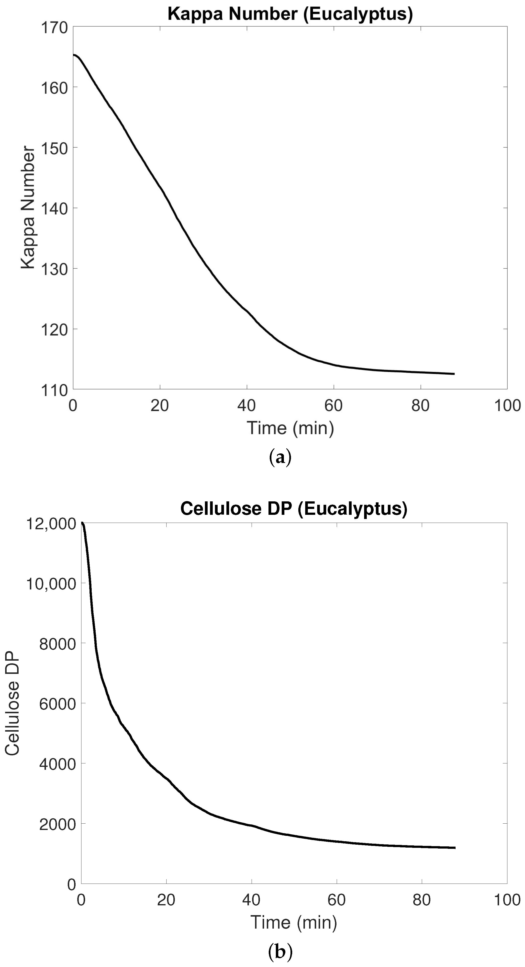
4.1. Multiscale Model

The multiscale model is used to predict the temporal evolution of wood chip properties as well as the spatiotemporal evolution of the kMC lattice at a temperature of 420 K and a NaOH concentration of 50 wt%. As shown in Figure 4, the orange, yellow, purple, and green sites represent lignin, cellulose, xylan, and galactoglucomman in the solid phase, respectively, while the blue sites represent the entrapped-liquor phase. As the solid components dissolve, the lignin and hemicellulose content in the chips fall significantly, and the entrapped-liquor content increases.
The prediction trends of the Kappa number and cellulose D P are shown in Figure 5. The Kappa number is seen to gradually decrease from 165 to 113 as delignification occurs in the wood chips, while the cellulose D P shows a sharp drop at the beginning of the pulping process and then achieves the equilibrium around 1600. To verify the accuracy of the multiscale model, it was validated against data of three different wood species: Date Palm Rachis, Pinus Radiata, and Eucalyptus [61,62,63]. The model was run at 413 K with a cooking time of 120 min and a NaOH concentration of 12 wt%, and the results are shown in Table 2.
It is seen that, for all three different wood species, the set-point values of the Kappa number and cellulose D P are similar to the values found in the literature [61,62,63], and the mean error is less than 10%. This suggests that the multiscale model is a valid virtual experiment for the batch pulp digester process, and can be used to generate data for varying operating conditions in order to train the LSTM-ANN model structure.
Remark 3. 
The results shown in Figure 5 are representative, and the trends of the Kappa number and D P for other input profiles follow a similar trend. It is assumed that the multiscale model remains effective under all these different operating conditions.

4.2. LSTM-ANN Model

Through optimization of the network structure, the best structure was obtained with three hidden layers, each containing 40 nodes. A batch size of 16 and a dropout rate of 0.5 were used as it was found that using a dropout layer in conjunction with the early stopping technique reduced the overfitting of the data [38]. The optimal network structure was chosen from several network configurations listed in Table 3 and includes an input layer, three LSTM layers, an ANN layer, a fully connected layer, an output layer, and a regression layer. The network configuration shown in the third row (Serial No. 3) was chosen as it showed a high R 2 value with a 0.5 dropout rate.
Remark 4. 
The listed network configurations are not a comprehensive set. During the process of hyperparameter tuning, a wide range of structures with a varying number of nodes, layers, types of activation functions, and dropout rates were considered.
The trained model was tested on 100 test datasets for accuracy evaluation. The parity plots between the multiscale model and LSTM-ANN model for the Kappa number and cellulose D P at the end of the pulping process are shown in Figure 6. An upper and lower bound of 10% was added to the bisector. The plot shows that the model was well-trained and had an average R 2 value of 0.9953 for the Kappa number and 0.9846 for cellulose D P .
In order to compare the accuracy when a deep neural network (DNN) was used instead of an LSTM to train the data with a combination of time-invariant and time-varying operating conditions, parity plots between the multiscale model and DNN model are shown in Figure 7. The R 2 values for the Kappa number and cellulose D P are seen to be very low (less than 0.8) despite the network structure having three layers with 40 hidden nodes each (the same number of total nodes as the LSTM model). This shows that the DNN was unable to capture the temporal dependencies as the LSTM did, and thus the aforementioned LSTM network structure was selected for further study. Next, the controller results are presented.

4.3. LSTM-ANN-Based MPC

As shown in the parity plots, the LSTM-ANN model effectively establishes a relationship between the operating conditions and the output set-point values. This LSTM-ANN model is then integrated into the MPC described in the previous section to obtain the optimal input profiles. These profiles are then used in the multiscale model to calculate the Kappa number and cellulose D P in an iterative manner at each time step. To demonstrate the controller’s capabilities, the desired set-point values of Kappa number = 90 and cellulose D P = 700 were set. Figure 8 shows the optimal input profiles for the cooking time, NaOH concentration, and the free-liquor temperature under MPC operation. As expected, the cooking time and NaOH concentration remained constant throughout the process, following the constraints set in Equations (21)–(22).
A cooking time of 80 min and a NaOH concentration of 62 wt% were obtained. The optimal free-liquor temperature profile also varied between 390 and 430 K with control actions being taken every 10 min. Figure 9 shows the output under MPC operation. It is seen that the cellulose D P drops quickly in value at the start and then stabilizes near the desired set-point value. The Kappa number steadily decreases over the course of the process, and attains a value close to the set-point value of 90. Thus, our framework demonstrated its capability to obtain optimal constant values for the cooking time and NaOH concentration in addition to a time-varying profile for the free-liquor temperature.
Remark 5. 
All the kMC simulations, MPC calculations, and neural network training were performed on a computer with an Intel Core i7–4770 CPU with 3.40 GHz and 16.0 GB RAM running on a Windows 10, 64-bit operating system using MATLAB 2022a. The multiscale model took around 10–15 min to run, while the LSTM-ANN model within the MPC could be executed within seconds. As control actions are taken every 10 min, this provides enough time for the user to adjust the operating conditions and rerun the MPC for the next iteration.

5. Conclusions

In conclusion, in this article, we presented the development of a layered multiscale model that integrates mass and energy balance equations from the extended Purdue model with a kMC algorithm to predict the temporal evolution of crucial paper properties, such as the Kappa number and cellulose D P . The model describes the degradation of wood chips associated with the dissolution of wood chip components and the depolymerization of cellulose due to alkaline hydrolysis, peeling-off, and stopping reactions. The multiscale model, which acts as a virtual experiment, was validated and then used offline with different sets of operating conditions to obtain a rich set of data for training the LSTM-ANN model with an R 2 value of over 0.98.
Finally, a closed-loop controller was designed using the LSTM-ANN-based neural network to obtain optimal profiles of operating conditions that are a combination of time-invariant inputs (such as the cooking time and NaOH concentration) and time-varying inputs (such as the free liquor temperature). The controller achieved target set-point values for the Kappa number and cellulose D P with minimal offset while considering process constraints. This trained LSTM-ANN model can, thus, be utilized in place of the complex first-principles model to significantly reduce the computation time while using an online controller.

Author Contributions

Conceptualization, P.S., H.-K.C. and J.S.-I.K.; methodology, P.S., H.-K.C. and J.S.-I.K.; software, P.S. and H.-K.C.; validation, P.S.; formal analysis, P.S., H.-K.C. and J.S.-I.K.; investigation, P.S. and J.S.-I.K.; resources, P.S., H.-K.C. and J.S.-I.K.; data curation, P.S. and H.-K.C.; writing—original draft preparation, P.S.; writing—review and editing, P.S. and J.S.-I.K.; visualization, P.S., H.-K.C. and J.S.-I.K.; supervision, J.S.-I.K.; project administration, J.S.-I.K.; funding acquisition, J.S.-I.K. All authors have read and agreed to the published version of the manuscript.

Funding

Financial support from the Texas A&M Energy Institute and the Artie McFerrin Department of Chemical Engineering is greatly acknowledged by the authors.

Data Availability Statement

The data presented in this study are available on request from the corresponding author. The data are not publicly available due to privacy reasons.

Conflicts of Interest

The authors declare no conflict of interest.

References

  1. VDP-Facts about Paper 2022. Available online: https://papertoexport.com/paper-consumption-worldwide-from-2020-to-2030-2/ (accessed on 10 January 2023).
  2. Tsai, W.H.; Lai, S.Y. Green production planning and control model with ABC under industry 4.0 for the paper industry. Sustainability 2018, 10, 2932. [Google Scholar] [CrossRef] [Green Version]
  3. Pätäri, S.; Tuppura, A.; Toppinen, A.; Korhonen, J. Global sustainability megaforces in shaping the future of the European pulp and paper industry towards a bioeconomy. For. Policy Econ. 2016, 66, 38–46. [Google Scholar] [CrossRef]
  4. Lawrence, A.; Karlsson, M.; Thollander, P. Effects of firm characteristics and energy management for improving energy efficiency in the pulp and paper industry. Energy 2018, 153, 825–835. [Google Scholar] [CrossRef]
  5. Singh, A.K.; Bilal, M.; Iqbal, H.M.; Meyer, A.S.; Raj, A. Bioremediation of lignin derivatives and phenolics in wastewater with lignin modifying enzymes: Status, opportunities and challenges. Sci. Total Environ. 2021, 777, 145988. [Google Scholar] [CrossRef] [PubMed]
  6. Choi, H.K.; Kwon, J.S.I. Modeling and control of cell wall thickness in batch delignification. Comput. Chem. Eng. 2019, 128, 512–523. [Google Scholar] [CrossRef]
  7. Choi, H.K.; Kwon, J.S.I. Multiscale modeling and multiobjective control of wood fiber morphology in batch pulp digester. AIChE J. 2020, 66, e16972. [Google Scholar] [CrossRef]
  8. Li, J.; Gellerstedt, G. On the structural significance of the kappa number measurement. Nord. Pulp Pap. Res. J. 1998, 13, 153–158. [Google Scholar] [CrossRef]
  9. Hart, P.W.; Colson, G.W.; Antonsson, S.; Hjort, A. Impact of impregnation on high kappa number hardwood pulps. BioResources 2011, 6, 5139–5150. [Google Scholar]
  10. Alves, A.; Santos, A.; da Silva Perez, D.; Rodrigues, J.; Pereira, H.; Simoes, R.; Schwanninger, M. NIR PLSR model selection for Kappa number prediction of maritime pine Kraft pulps. Wood Sci. Technol. 2007, 41, 491–499. [Google Scholar] [CrossRef]
  11. Gurnagul, N.; Page, D.H.; Paice, M.G. The effect of cellulose degradation on the strength of wood pulp fibres. Nord. Pulp Pap. Res. J. 1992, 7, 152–154. [Google Scholar] [CrossRef]
  12. Karak, T.; Bhagat, R.; Bhattacharyya, P. Municipal solid waste generation, composition, and management: The world scenario. Crit. Rev. Environ. Sci. Technol. 2012, 42, 1509–1630. [Google Scholar] [CrossRef]
  13. Haile, A.; Gelebo, G.G.; Tesfaye, T.; Mengie, W.; Mebrate, M.A.; Abuhay, A.; Limeneh, D.Y. Pulp and paper mill wastes: Utilizations and prospects for high value-added biomaterials. Bioresour. Bioprocess. 2021, 8, 1–22. [Google Scholar] [CrossRef]
  14. Fang, Z.; Li, B.; Liu, Y.; Zhu, J.; Li, G.; Hou, G.; Zhou, J.; Qiu, X. Critical role of degree of polymerization of cellulose in super-strong nanocellulose films. Matter 2020, 2, 1000–1014. [Google Scholar] [CrossRef]
  15. De Silva, R.; Byrne, N. Utilization of cotton waste for regenerated cellulose fibres: Influence of degree of polymerization on mechanical properties. Carbohydr. Polym. 2017, 174, 89–94. [Google Scholar] [CrossRef] [PubMed]
  16. Carvalho, M.; Ferreira, P.; Figueiredo, M. Cellulose depolymerisation and paper properties in E. globulus kraft pulps. Cellulose 2000, 7, 359–368. [Google Scholar] [CrossRef]
  17. Rasi, M. Permeability properties of paper materials. In Research Report/Department of Physics; University of Jyväskylä: Jyväskylä, Finland, 2013. [Google Scholar]
  18. Abdelmouleh, M.; Boufi, S.; Belgacem, M.N.; Dufresne, A.; Gandini, A. Modification of cellulose fibers with functionalized silanes: Effect of the fiber treatment on the mechanical performances of cellulose–thermoset composites. J. Appl. Polym. Sci. 2005, 98, 974–984. [Google Scholar] [CrossRef]
  19. Gustafson, R.R.; Sleicher, C.A.; McKean, W.T.; Finlayson, B.A. Theoretical model of the kraft pulping process. Ind. Eng. Chem. Process Des. Dev. 1983, 22, 87–96. [Google Scholar] [CrossRef] [Green Version]
  20. Andersson, N.; Wilson, D.I.; Germgård, U. An improved kinetic model structure for softwood kraft cooking. Nord. Pulp Pap. Res. J. 2003, 18, 200–209. [Google Scholar] [CrossRef]
  21. Christensen, T. A mathematical Model of the Kraft Pulping Process; Purdue University: West Lafayette, IN, USA, 1982. [Google Scholar]
  22. Bhartiya, S.; Dufour, P.; Doyle III, F.J. Fundamental thermal-hydraulic pulp digester model with grade transition. AIChE J. 2003, 49, 411–425. [Google Scholar] [CrossRef] [Green Version]
  23. Choi, H.K.; Kwon, J.S.I. Multiscale modeling and control of Kappa number and porosity in a batch-type pulp digester. AIChE J. 2019, 65, e16589. [Google Scholar] [CrossRef]
  24. Son, S.H.; Choi, H.K.; Kwon, J.S.I. Multiscale modeling and control of pulp digester under fiber-to-fiber heterogeneity. Comput. Chem. Eng. 2020, 143, 107117. [Google Scholar] [CrossRef]
  25. Pahari, S.; Bhadriraju, B.; Akbulut, M.; Kwon, J.S.I. A slip-spring framework to study relaxation dynamics of entangled wormlike micelles with kinetic Monte Carlo algorithm. J. Colloid Interface Sci. 2021, 600, 550–560. [Google Scholar] [CrossRef] [PubMed]
  26. Andersen, M.; Panosetti, C.; Reuter, K. A practical guide to surface kinetic Monte Carlo simulations. Front. Chem. 2019, 7, 202. [Google Scholar] [CrossRef] [PubMed]
  27. Son, S.H.; Choi, H.K.; Kwon, J.S.I. Application of offset-free Koopman-based model predictive control to a batch pulp digester. AIChE J. 2021, 67, e17301. [Google Scholar] [CrossRef]
  28. Son, S.H.; Choi, H.K.; Moon, J.; Kwon, J.S.I. Hybrid Koopman model predictive control of nonlinear systems using multiple EDMD models: An application to a batch pulp digester with feed fluctuation. Control Eng. Pract. 2022, 118, 104956. [Google Scholar] [CrossRef]
  29. Dobbelaere, M.R.; Plehiers, P.P.; Van de Vijver, R.; Stevens, C.V.; Van Geem, K.M. Machine learning in chemical engineering: Strengths, weaknesses, opportunities, and threats. Engineering 2021, 7, 1201–1211. [Google Scholar] [CrossRef]
  30. Venkatasubramanian, V. The promise of artificial intelligence in chemical engineering: Is it here, finally? AIChE J. 2018, 65, 466–478. [Google Scholar] [CrossRef] [Green Version]
  31. Bhadriraju, B.; Narasingam, A.; Kwon, J.S.I. Machine learning-based adaptive model identification of systems: Application to a chemical process. Chem. Eng. Res. Des. 2019, 152, 372–383. [Google Scholar] [CrossRef]
  32. Pahari, S.; Moon, J.; Akbulut, M.; Hwang, S.; Kwon, J.S.I. Estimation of microstructural properties of wormlike micelles via a multi-scale multi-recommendation batch bayesian optimization. Ind. Eng. Chem. Res. 2021, 60, 15669–15678. [Google Scholar] [CrossRef]
  33. Yu, Y.; Si, X.; Hu, C.; Zhang, J. A review of recurrent neural networks: LSTM cells and network architectures. Neural Comput. 2019, 31, 1235–1270. [Google Scholar] [CrossRef]
  34. Hochreiter, S.; Schmidhuber, J. Long short-term memory. Neural Comput. 1997, 9, 1735–1780. [Google Scholar] [CrossRef]
  35. Thompson, M.L.; Kramer, M.A. Modeling chemical processes using prior knowledge and neural networks. AIChE J. 1994, 40, 1328–1340. [Google Scholar] [CrossRef]
  36. Prasad, V.; Bequette, B.W. Nonlinear system identification and model reduction using artificial neural networks. Comput. Chem. Eng. 2003, 27, 1741–1754. [Google Scholar] [CrossRef]
  37. Jeon, B.K.; Kim, E.J. LSTM-based model predictive control for optimal temperature set-point planning. Sustainability 2021, 13, 894. [Google Scholar] [CrossRef]
  38. Wu, Z.; Rincon, D.; Luo, J.; Christofides, P.D. Machine learning modeling and predictive control of nonlinear processes using noisy data. AIChE J. 2021, 67, e17164. [Google Scholar] [CrossRef]
  39. Shah, P.; Sheriff, M.Z.; Bangi, M.S.F.; Kravaris, C.; Kwon, J.S.I.; Botre, C.; Hirota, J. Deep neural network-based hybrid modeling and experimental validation for an industry-scale fermentation process: Identification of time-varying dependencies among parameters. Chem. Eng. J. 2022, 441, 135643. [Google Scholar] [CrossRef]
  40. Choi, H.K.; Kwon, J.S.I. Multiscale modeling and control of fiber length in pulp digester. In Proceedings of the 2020 American Control Conference (ACC), Denver, CO, USA, 1–3 July 2020; pp. 4343–4348. [Google Scholar]
  41. Jung, J.; Choi, H.K.; Son, S.H.; Kwon, J.S.I.; Lee, J.H. Multiscale modeling of fiber deformation: Application to a batch pulp digester for model predictive control of fiber strength. Comput. Chem. Eng. 2022, 158, 107640. [Google Scholar] [CrossRef]
  42. Irle, M.A.; Barbu, M.C.; Reh, R.; Bergland, L.; Rowell, R.M. 10 Wood Composites. Handb. Wood Chem. Wood Compos. 2012, 321–411. [Google Scholar] [CrossRef]
  43. Van Loon, L.; Glaus, M. Review of the kinetics of alkaline degradation of cellulose in view of its relevance for safety assessment of radioactive waste repositories. J. Environ. Polym. Degrad. 1997, 5, 97–109. [Google Scholar] [CrossRef] [Green Version]
  44. Pavasars, I.; Hagberg, J.; Borén, H.; Allard, B. Alkaline degradation of cellulose: Mechanisms and kinetics. J. Polym. Environ. 2003, 11, 39–47. [Google Scholar] [CrossRef]
  45. Kim, D.; Kim, M.; Kim, W. Wafer edge yield prediction using a combined long short-term memory and feed-forward neural network model for semiconductor manufacturing. IEEE Access 2020, 8, 215125–215132. [Google Scholar] [CrossRef]
  46. Kowsher, M.; Tahabilder, A.; Sanjid, M.Z.I.; Prottasha, N.J.; Uddin, M.S.; Hossain, M.A.; Jilani, M.A.K. LSTM-ANN & BiLSTM-ANN: Hybrid deep learning models for enhanced classification accuracy. Procedia Comput. Sci. 2021, 193, 131–140. [Google Scholar]
  47. Makris, D.; Kaliakatsos-Papakostas, M.; Karydis, I.; Kermanidis, K.L. Combining LSTM and feed forward neural networks for conditional rhythm composition. In Proceedings of the International Conference on Engineering Applications of Neural Networks; Springer: Athens, Greece, 2017; pp. 570–582. [Google Scholar]
  48. Feng, C.; Chang, L.; Li, C.; Ding, T.; Mai, Z. Controller optimization approach using LSTM-based identification model for pumped-storage units. IEEE Access 2019, 7, 32714–32727. [Google Scholar] [CrossRef]
  49. Schwedersky, B.B.; Flesch, R.C.; Dangui, H.A. Practical nonlinear model predictive control algorithm for long short-term memory networks. IFAC-PapersOnLine 2019, 52, 468–473. [Google Scholar] [CrossRef]
  50. Gers, F.A.; Schmidhuber, J.; Cummins, F. Learning to forget: Continual prediction with LSTM. Neural Comput. 2000, 12, 2451–2471. [Google Scholar] [CrossRef] [PubMed]
  51. Greff, K.; Srivastava, R.K.; Koutník, J.; Steunebrink, B.R.; Schmidhuber, J. LSTM: A search space odyssey. IEEE Trans. Neural Netw. Learn. Syst. 2016, 28, 2222–2232. [Google Scholar] [CrossRef] [Green Version]
  52. Graves, A.; Schmidhuber, J. Framewise phoneme classification with bidirectional LSTM and other neural network architectures. Neural Netw. 2005, 18, 602–610. [Google Scholar] [CrossRef] [PubMed]
  53. Kingma, D.P.; Ba, J. Adam: A method for stochastic optimization. arXiv 2014, arXiv:1412.6980. [Google Scholar]
  54. Bergstra, J.; Bardenet, R.; Bengio, Y.; Kégl, B. Algorithms for hyper-parameter optimization. Adv. Neural Inf. Process. Syst. 2011, 24, 2546–2554. [Google Scholar]
  55. Shah, P.; Sheriff, M.Z.; Bangi, M.S.F.; Kravaris, C.; Kwon, J.S.I.; Botre, C.; Hirota, J. Multi-rate observer design and optimal control to maximize productivity of an industry-scale fermentation process. AIChE Journal 2022, 69, e17946. [Google Scholar] [CrossRef]
  56. Narasingam, A.; Kwon, J.S. Development of local dynamic mode decomposition with control: Application to model predictive control of hydraulic fracturing. Comput. Chem. Eng. 2017, 106, 501–511. [Google Scholar] [CrossRef]
  57. Pahari, S.; Moon, J.; Akbulut, M.; Hwang, S.; Kwon, J.S.I. Model predictive control for wormlike micelles (WLMs): Application to a system of CTAB and NaCl. Chem. Eng. Res. Des. 2021, 174, 30–41. [Google Scholar] [CrossRef]
  58. Zarzycki, K.; Ławryńczuk, M. LSTM and GRU neural networks as models of dynamical processes used in predictive control: A comparison of models developed for two chemical reactors. Sensors 2021, 21, 5625. [Google Scholar] [CrossRef] [PubMed]
  59. Yunpeng, L.; Di, H.; Junpeng, B.; Yong, Q. Multi-step ahead time series forecasting for different data patterns based on LSTM recurrent neural network. In Proceedings of the 2017 14th web information systems and applications conference (WISA), Liuzhou, China, 11–12 November 2017; pp. 305–310. [Google Scholar]
  60. Sagheer, A.; Kotb, M. Time series forecasting of petroleum production using deep LSTM recurrent networks. Neurocomputing 2019, 323, 203–213. [Google Scholar] [CrossRef]
  61. Khiari, R.; Mhenni, M.; Belgacem, M.; Mauret, E. Chemical composition and pulping of date palm rachis and Posidonia oceanica–A comparison with other wood and non-wood fibre sources. Bioresour. Technol. 2010, 101, 775–780. [Google Scholar] [CrossRef] [PubMed]
  62. Mishra, S. Bleaching of Cellulosic Paper Fibres with Ozone-Effect on the Fibre Properties; Institut Polytechnique de Grenoble: Grenoble, France, 2010. [Google Scholar]
  63. Mansouri, S.; Khiari, R.; Bendouissa, N.; Saadallah, S.; Mhenni, F.; Mauret, E. Chemical composition and pulp characterization of Tunisian vine stems. Ind. Crop. Prod. 2012, 36, 22–27. [Google Scholar] [CrossRef]
Figure 1. Worldwide paper consumption prediction volume.
Processes 11 00809 g001
Figure 2. Schematic illustration of a pulp digester composed of three phases (solid, entrapped-liquor, and free-liquor). Reproduced with permission of the American Automatic Control Council for the conference article [40].
Processes 11 00809 g002
Figure 3. Architecture of the LSTM-ANN network.
Processes 11 00809 g003
Figure 4. Graphical illustration of the simulation lattice at t = 0 and t = 87.84 min.
Processes 11 00809 g004
Figure 5. (a) The Kappa number predicted by the multiscale kMC model for Eucalyptus wood and (b) the degree of polymerization predicted by the multiscale kMC model for Eucalyptus wood.
Processes 11 00809 g005
Figure 6. (a) Parity plot for the Kappa number prediction for the test data (100 datasets) at the end of the pulping process t = t e n d with the LSTM-ANN model and (b) parity plot for D P prediction for the test data (100 datasets) at the end of the pulping process t = t e n d with the LSTM-ANN model.
Processes 11 00809 g006
Figure 7. (a) Parity plot for the Kappa number prediction for the test data (100 datasets) at t = t e n d with the DNN model and (b) parity plot for D P prediction for the test data (100 datasets) at t = t e n d with the DNN model.
Processes 11 00809 g007
Figure 8. Optimal input profiles and bounds for the cooking time, NaOH concentration, and free-liquor temperature as obtained from the closed-loop simulation.
Processes 11 00809 g008
Figure 9. Trajectories of the Kappa number and degree of polymerization as obtained from the closed-loop simulation.
Processes 11 00809 g009
Table 1. Probability distribution for cellulose depolymerization.
ProbabilitiesDepolymerization Mechanism
  0 < ξ R P R P + R S + R H       Peeling-off (Null event)
  R P R P + R S + R H < ξ R P + R S R P + R S + R H Stopping (Null event)
R P + R S R P + R S + R H < ξ 1 Cellulose chain scission event
Table 2. A comparison of the cellulose D P and Kappa number between the experimental data and model simulation at the end of the pulping process ( t = t e n d ) for three different wood species [61,62,63].
SpeciesCellulose DP Kappa Number
ExperimentModelExperimentModel
Eucalyptus139913428.711.4
Date Palm Rachis120311745452.6
Pinus Radiata1423136810.610.8
Mean error4%Mean error8%
Table 3. List of configurations for the LSTM network.
Serial No.LayersNodesBatch SizeDropout Rate R 2 Kappa R 2 DP
1220160.20.9420.884
2240320.40.9570.901
3340160.50.9950.985
4320320.20.9820.944
53403200.9980.992
63101600.9750.954
7340160.80.9260.895
Disclaimer/Publisher’s Note: The statements, opinions and data contained in all publications are solely those of the individual author(s) and contributor(s) and not of MDPI and/or the editor(s). MDPI and/or the editor(s) disclaim responsibility for any injury to people or property resulting from any ideas, methods, instructions or products referred to in the content.

