Data-Driven Prediction of Li-Ion Battery Degradation Using Predicted Features

Abstract

For their emergent application in electric vehicles, the development of fast and accurate algorithms to monitor the health status of batteries and aid decision-making in relation to maintenance and replacement is now of paramount importance. Data-driven approaches are preferred due to the difficulties associated with defining valid models for system and parameter identification. In recent years, the use of features to enhance data-driven methods has become commonplace. Unless the data sets are from multiple batteries, however, such approaches cannot be used to predict more than one cycle ahead because the features are unavailable for future cycles, in the absence of different embedding strategies. In this paper, we propose a novel approach in which features are predicted for future cycles, enabling predictions of the state of health for an arbitrary number of cycles ahead, and, therefore, predictions for the end-of-life. This is achieved by using a data-driven approach to predict voltage and temperature curves for future cycles, from which important signatures of degradation can be extracted and even used directly for degradation predictions. The use of features is shown to enhance the state-of-health predictions. The approach we develop is capable of accurate predictions using a data set specific to the battery under consideration. This avoids the need for large multi-battery data sets, which are hampered by natural variations in the performance and degradation of batteries even from the same batch, compromising the prediction accuracy of approaches based on such data.

1. Introduction

Lithium-ion batteries (LiBs) have a long history of use in the portable electronics sector, and have become the de-facto technology for battery electric vehicles. During use, LiBs undergo various electrochemical and mechanical degradation mechanisms [1]. Over repeated cycles of charge and discharge, therefore, the batteries inevitably suffer an irreversible loss in capacity. Not only does this incur costs in terms of maintenance and replacement, but sudden catastrophic failures caused by degradation can also lead to much more severe consequences. The development of accurate algorithms to facilitate battery management, monitor their health status and aid decision-making in relation to replacement has therefore become of paramount importance [1,2,3].

To quantify the gradual decay in the maximum available capacity, the state-of-health (SOH), namely the ratio (or percentage) of available capacity for full discharge compared to the rated capacity, is used. A criterion is then defined for when the battery is deemed unfit for its current application, normally when the battery SOH falls below a threshold value. This criterion defines the so-called end-of-life (EOL), at which point it may be used for a secondary (second-life) application [4]. A related concept is the remaining useful life (RUL), which is the number of cycles remaining before EOL is reached.

Predicting the rate of degradation in LIBs is far from trivial since the processes that lead to degradation are not entirely understood and are difficult to measure, which compromises the accuracy and applicability of detailed physics-based models. An early popular approach, which continues to be adopted, is based on semi-empirical or empirical models. Examples include equivalent electrical circuit models linking the circuit parameters to the SOH [5], and models fitting data to various parameter-dependent functions [6,7]. Classical state-space models for time series can be used to enhance these methods, e.g., the combination of an equivalent circuit model with a Kalman filter to account for drift in the circuit parameters that are used to estimate the SOH [8], which can be further improved upon with a Bayesian filter [9].

The difficulties associated with defining valid models for system and parameter identification have led to a growth in purely data-driven or machine-learning methods (see [10] and [11] for recent reviews). The main methods are artificial neural networks (ANNs), deep networks (DNNs) [12,13,14], Gaussian process (GP) models [15,16], and support vector regression (SVR) [17,18]. Other methods, including Hidden Markov Models (HMM) [19] and k-nearest neighbor (k-NN) regression [20], have also been employed.

In particular, DNNs, which are defined as ANNs with more than one hidden layer, have emerged as a popular choice, with a plethora of different architectures, including recurrent networks (RNNs), such as the Long Short Term Memory (LSTM) network [21,22], convolutional networks (CNN) [23], and hybrid architectures such as a CNN-LSTM [24] or gated recurrent unit-CNN (GRU-CNN) [25]. Another popular approach to predicting the SOH or RUL is GP modelling [16]. GP models have some advantages over non-Bayesian approaches such as ANNs and SVR; namely, a natural measure of predictive uncertainty and the requirement in general of fewer training samples (due to the smaller number of (hyper)parameters).

ML methods have almost exclusively been applied to the estimation of the SOH, RUL, or EOL, with very few exceptions, such as the prediction of voltage-discharge capacity curves in [26]. Data sets often contain information beyond voltage-current curves, such as temperature measurements and impedance data. Various signatures of degradation can be extracted from this data, such as the slope of the charge or discharge curve at selected points in the cycle, or the maximum voltage on charge. It is tempting to incorporate such features as inputs to improve predictions [27,28], and in recent years such an approach has become commonplace. The features can be designed by hand or learned from the raw data as part of the algorithm. It has been demonstrated that a number of physical features are highly correlated to the degradation, e.g., the slope of the voltage curves at the beginning or end of charge, or the maximum temperature reached during charge [27,28,29].

Qian et al. [23] used randomly selected segments of the charge voltage, differential charge voltage, and charge current curves as inputs to a CNN, training on multiple battery data sets. Their model was designed to predict the capacity for unseen batteries of the same type, under the same cycling conditions. Similar approaches were adopted to predict the EOL by Severson et al. using linear regression [30], by Hong et al. [31] using a CNN, and by Hsu et al. [26] using a highly complex DNN that learns features from charge-discharge data in the first layer to predict the EOL and RUL. Zhang et al. [32] used a GP model into which electrochemical impedance measurements from the current cycle were fed as inputs to predict the capacity.

The advantage of such models, based on multi-battery data sets, is the capability to utilize existing information, possibly under different charge-discharge policies and operating conditions, in order to make early predictions. In [26,31], only a small number of charge-discharge input cycles are required for ballpark predictions. The disadvantages of this approach are that it requires very large data sets and that natural variabilities in the performance and degradation across batteries from the same batch, even under the same charge-discharge policies and operating conditions, can lead to inaccurate predictions for a new battery. As Severson et al. state, such models are suitable for situations in which very early predictions are required, but in which the accuracy is not critical, e.g., sorting/grading and pack design applications [30].

The majority of machine learning models focus on predicting the SOH, RUL, or EOL using data originating from the battery under consideration, which does not require a large data set and is less prone to inaccuracies due to the aforementioned variabilities. Yang et at. [27] used hand-crafted physical features such as the time for a constant current charge and the slope of the voltage profile at the end of charge as inputs to a GP model. A similar approach was adopted by Chen et al. [29] using an RNN with up to 20 physical features. Tagade et al. [33] used a deep GP with randomly extracted sequences of time, voltage, and temperature (on either discharge or charge) as inputs. The nonlinear autoregression with exogenous input (NARX) model of Khaleghi et al. [34] uses randomly selected charge voltage sequences of specified lengths.

The use of features in this way, training on a specific data set for online use with information from a battery management system (BMS), cannot, however, be applied recursively, in contrast to standard one-step autoregressive models in which features are not included [35]. We note that the capacity model of Zhang et al. [32] suffers from the same issue in the way that it is applied. The features become available to use as inputs one cycle at a time, which means that to obtain multi-step lookahead predictions these models must be used in a direct time series approach, which has massive additional computational costs (m separate models for m steps ahead), or else modified into sequence-to-sequence models, in which a sequence of future capacity values are predicted from a sequence of inputs/features.

In this paper, we adopt a different and novel approach that overcomes this limitation. We first predict the voltage, temperature, and time sequences on discharge or charge. Any other quantities feasibly available from an onboard BMS can also be included. We consider two data sets, with one containing voltage measurements, and the other containing, voltage, temperature, and impedance measurements. The impedance results contained a significant degree of noise and were therefore excluded. In general, impedance data would not be available in-situ from a standard BMS, so we do not consider their inclusion to be practical. We predict the voltage and (if available) temperature curves for future cycles, from which we extract predicted features multiple cycles ahead. We use these features in a GP approach to predict the SOH, demonstrating significant improvements over a standard GP approach that uses only the cycle number as the input.

We compare the accuracy of our method with other methods in the literature that employ the same data sets. We also investigate the effects of noise in the data sets, since inevitably some level of noise will be present. Moreover, from the predicted voltage and temperature curves, other signatures of degradation can be obtained directly. In contrast to other feature engineering approaches based on a single battery data set, our method can be used for a multi-step lookahead analysis to predict the EOL and RUL.

2. Methods

2.1. Data Sets

We employed the NASA data set of Saha et al. [36], in which batteries (labeled B0005, B0006, B0007, and B0018) were repeatedly cycled at constant current. Impedance measurements were taken at various (non-regular) cycles. All experiments were conducted at room temperature.

The batteries were charged at a constant current of 1.5 A to a voltage of 4.2 V followed by a constant voltage (CV) mode until the current reached 20mA. They were then discharged at a constant current of 2 A until the battery voltage fell to 2.7 V, 2.5 V, 2.2 V, and 2.5 V for B0005, B0006, B0007, and B0018, respectively. Impedance measurements using electrochemical impedance spectroscopy (EIS) were taken at various cycles with a frequency sweep from 0.1 Hz to 5 kHz.

The batteries were cycled as above until they reached end-of-life (EOL), defined as a 30% fade compared to the rated capacity (from 2 Ahr to 1.4 Ahr). The voltage, current, and temperature were measured throughout cycling, with a non-constant number of sampling times. For example, there were between 179 and 354 sampling times for battery B0005, depending on the cycle number, and similarly for the other batteries. The capacity was estimated at the end of discharge for each cycle. For certain cycles, the sense current, battery current, current ratio, battery impedance, rectified impedance, calibrated and smoothed battery impedance, estimated electrolyte resistance, and estimated charge transfer resistance was recorded from EIS.

For B0005, B0006, and B0007 there were a total of 168 charge-discharge cycles, while for B0018 there were 132 cycles. The impedance measurements contained a high level of noise, and were not therefore used in this study. We focus on the discharge profiles for B0006, B0007, and B0018; specifically, the voltage, temperature, time and capacity.

We also used the data set in [37], in which 130 different Li-ion batteries are repeatedly cycled under different load patterns and temperatures. In contrast to the older data set of [36], most of the cells exhibit a smoothly varying capacity. The batteries used were LiNi${}_{0.86}$Co${}_{0.11}$Al${}_{0.03}$O${}_2$ positive electrode (NCA) batteries, LiNi${}_{0.83}$Co${}_{0.11}$Mn${}_{0.07}$O${}_2$ positive electrode (NCM) batteries, and batteries with a blend of 42 wt.% Li(NiCoMn)O${}_2$ and 58 wt.% Li(NiCoAl)O${}_2$ for the positive electrodes. The rated capacities of the first 2 are 3.5 Ah and the rated capacity of the third is 2.5 Ah.

The batteries were cycled at 25, 35, or 45 C in a temperature-controlled chamber. A constant charge current ranging from 0.875 A to 10 A was used, until the cell voltage reached 4.2 V, followed by a constant voltage charge until the current reached 0.05 C (1C = 3.5 A or 2.5 A). The batteries were then discharged at a constant current between 0.875 A and 10 A to a voltage of 2.65 V for the NCA batteries and 2.5 V for the other batteries. Repeated cycling was carried out until the capacities fell to 71% of the rated values. The number of cycles, in this case, was typically much higher, reaching up to 1500 cycles. For each cycle, the charge and discharge voltage curves were recorded (there are no temperature or EIS measurements), together with the capacity at the end of each cycle.

2.2. Data Preprocessing

The raw data was pre-processed via the following steps:

1.

Cut off. In all discharge cycles, the voltage and (if available) temperature sequences for each cycle were truncated at the time when the voltage reached the cut off value.

2.

Interpolation. After cutting off, the data contained different numbers of measurements at different times from cycle to cycle. In order to obtain data on a fixed grid with the same number of values for each cycle n, we used interpolation to fit the voltage and temperature (if it is available) to smooth curves on each cycle. Using the interpolating polynomial, we then extracted 200 values for the voltage and temperature at equally spaced points in time, for each discharge curve .

The method we used was cubic splines $s_i(t)$, $i=1,\dots ,M_t$, where $M_t+1$ is the number of measurements in the cycle, at times $t_i$, $i=0,\dots ,M_t$. The interpolating polynomial is $s(t)=s_i(t)$, $t\in [t_{i-1},t_i]$, $i=1,\dots ,M_t$, with the condition that $s(t_i)=y(t_i)$, $i=0,\dots ,M_t$, where $y(t)$ is the voltage or temperature. $s(t)$ must be twice continuously differentiable and natural boundary conditions $s^{\prime \prime }(t_0)=s^{\prime \prime }(t_{M_t})=0$ were imposed to complete the specification for the coefficients in the splines.

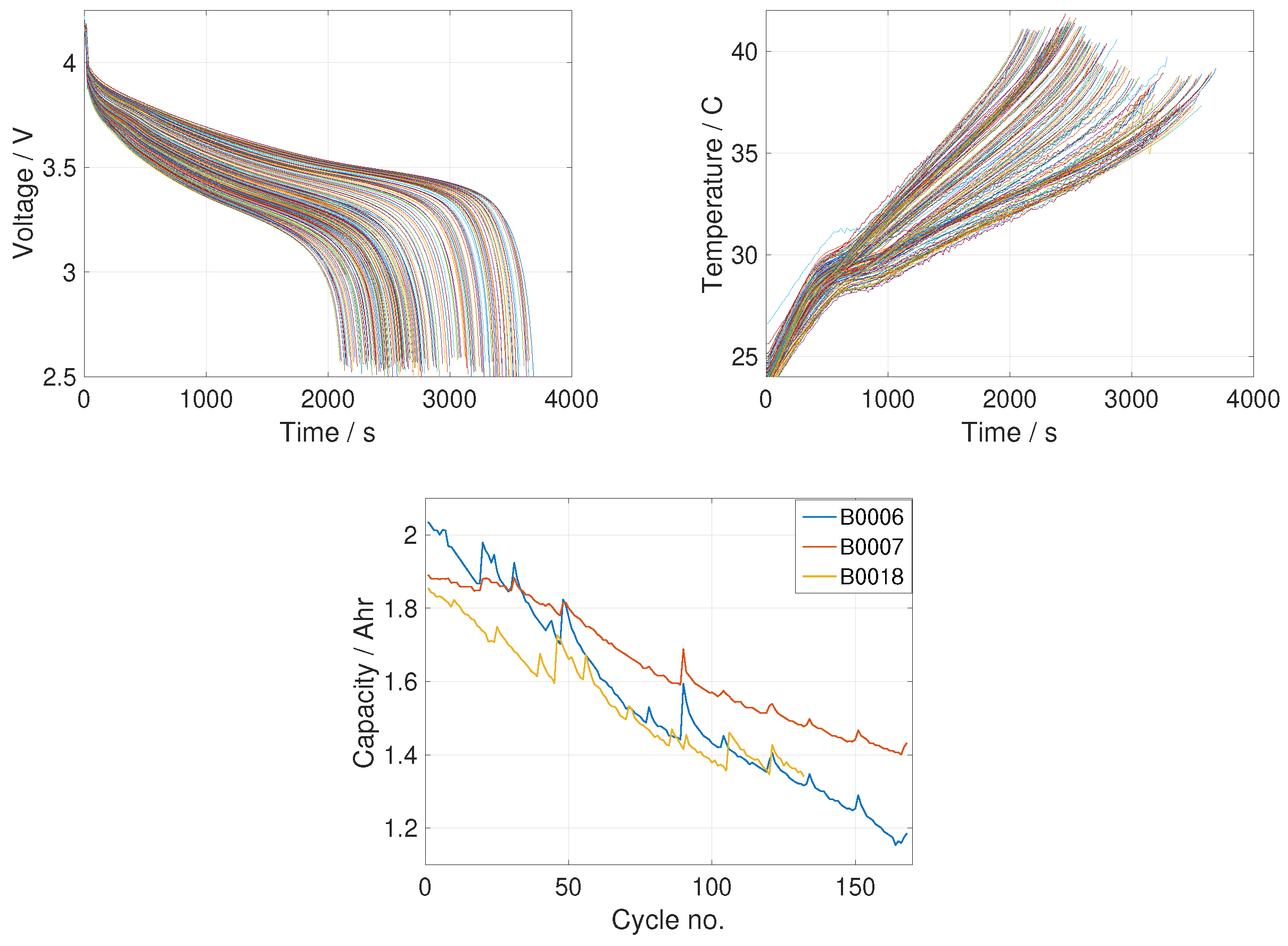
We vectorized the 200 values of voltage and temperature on each cycle to obtain vectors ${\mathbf{y}}_V(n)$, ${\mathbf{y}}_T(n)$, $n=1,\dots ,N$, respectively, where N is the number of cycles for the battery. The time sequence for cycle n is defined entirely by the time interval (200 equally spaced times), $\delta t(n)$, $n=1,\dots ,N$. The temperature and voltage after interpolation for the B0006 NASA battery, together with the measured capacity for all NASA batteries considered are shown in Figure 1.

2.3. Gaussian Process Models

We are provided with training data $\delta t(n)$, ${\mathbf{y}}_V(n)$ and ${\mathbf{y}}_T(n)$, $n=1,\dots ,N$, in which n denotes the cycle number, ${\mathbf{y}}_V(n)\in {\mathbb{R}}^d$ and ${\mathbf{y}}_T(n)\in {\mathbb{R}}^d$ represent sequences of d voltage and temperature values, respectively, and $\delta t(n)\in \mathbb{R}$ is a uniform interval between times at which the voltage/temperature values are recorded. We consider voltage and temperature to be different tasks and for an arbitrary n, we define the 2-dimensional array $\mathbf{Y}(n)\in {\mathbb{R}}^{d\times 2}$ that places the values at different time instances along the first dimension and the tasks along the second dimension. We can also organize the data points into a multi-dimensional array $\mathcal{Y}\in {\mathbb{R}}^{d\times 2\times N}$, in which the third dimension collects the values of $\mathbf{Y}(n)$ at the $n=1,\dots ,N$, cycles.

$\mathbf{Y}(n)$ is treated as a random process that can be approximated with a GP model. To this end, we place the following matrix prior over $\mathbf{Y}(n)$, which assumes a separable form:

$$\begin{array}{c}\mathrm{v}\mathrm{e}\mathrm{c}(\mathbf{Y}(n))\sim \mathcal{GP}(vec(\mathbf{Y}(n))\mid \mathbf{0},k_{\mathbf{Y}}(n,n^{\prime }|{\theta }_{\mathbf{Y}})\otimes C_d\otimes C_2+\delta (n,n^{\prime }){\tau }_{\mathbf{Y}}\otimes \mathbf{I})\hfill \end{array}$$

(1)

in which $\mathcal{GP}(·\mid ·,·)$ denotes a GP over the first argument, with the second and third arguments denoting the mean function and cross-covariance (kernel) function. $\mathrm{vec}(\mathbf{Y}(n))={({\mathbf{y}}_V{(n)}^T{\mathbf{y}}_T{(n)}^T)}^T\in {\mathbb{R}}^{2d}$ is a stacking of the mode 1 fibers (a vectorization), $\mathbf{I}$ is the identity matrix, $C_2\in {\mathbb{R}}^{2\times 2}$ is an unknown variance-covariance matrix between tasks, $C_d\in {\mathbb{R}}^{d\times d}$ is an unknown variance-covariance matrix between the components of ${\mathbf{y}}_V(n)$ and ${\mathbf{y}}_T(n)$, ⊗ is the Kronecker product and $\delta (n,n^{\prime })$ is the Kronecker-delta function. The mean is taken to be identically zero by virtue of centering the data.

The matrix/tensor GP covariance structure is separable by definition, which makes it a tractable and efficient model in terms of training and making predictions. Correlations across the cycle number n are embodied in the covariance function $k_{\mathbf{Y}}(n,n^{\prime }|{\theta }_{\mathbf{Y}})$. For any finite number of cycles, the covariance matrix for $\mathbf{Y}$ takes the form ${\mathbf{K}}_{\mathbf{Y}}\otimes C_d\otimes C_2$, in which ${\left[{\mathbf{K}}_{\mathbf{Y}}\right]}_{n{n}^{\prime }}=k_{\mathbf{Y}}(n,n^{\prime }|{\theta }_{\mathbf{Y}})$, $n,n^{\prime }=1,\dots ,N$. The covariance function (kernel) $k_{\mathbf{Y}}(n,n^{\prime }|{\theta }_{\mathbf{Y}})$ is dependent on unknown hyperparameters ${\theta }_{\mathbf{Y}}$, which must be inferred during training. The noise term $\delta (n,n^{\prime }){\tau }_{\mathbf{Y}}\otimes \mathbf{I}$ accounts for independent and identically distributed (i.i.d.) noise, or, equivalently, acts as a regularization term to prevent ill-conditioning. The signal variance ${\tau }_{\mathbf{Y}}$ is also an unknown hyperparameter. Formally, the model for the data point $\mathbf{Y}(n)$ is:

$$\mathbf{Y}(n)={\mathbf{Y}}_l(n)+\mathbf{E}(n),n=1,\dots ,N$$

(2)

in which ${\mathbf{Y}}_l(n)$ is an underlying latent function (evaluated at cycle n) corrupted by noise $\mathbf{E}(n)\in {\mathbb{R}}^{d\times 2}$, with prior distributions $\mathrm{vec}({\mathbf{Y}}_l(n))\sim \mathcal{GP}(\mathrm{vec}({\mathbf{Y}}_l(n))\mid \mathbf{0},k_{\mathbf{Y}}(n,n^{\prime }|{\theta }_{\mathbf{Y}})\otimes C_d\otimes C_2)$ and $\mathrm{vec}(\mathbf{E}(n))\sim \mathcal{GP}(\mathrm{vec}(\mathbf{E}(n))\mid \mathbf{0},\delta (n,n^{\prime }){\tau }_{\mathbf{Y}}\otimes \mathbf{I})$. That is, ${\mathbf{Y}}_l(n)$ is the real target of interest.

There are several main choices for the kernel function, and some of the most common are the squared exponential (SE) kernel, the linear kernel, the Matérn class of kernels, and the periodic kernel [38]:

$$\begin{array}{cc}\hfill k(n,n^{\prime }|\theta )& ={\theta }_{0}exp\left(-r^2\right),r=\sqrt{{\theta }_1{(n-n^{\prime })}^2}\hfill \end{array}$$

(3a)

$$\begin{array}{cc}\hfill k(n,n^{\prime })& ={\theta }_{0}n{n}^{\prime }\hfill \end{array}$$

(3b)

$$\begin{array}{cc}\hfill k(n,n^{\prime };\mathbf{\theta })& ={\theta }_0{f}_{\nu }(r)exp\left(-\sqrt{\nu }r\right)\hfill \end{array}$$

(3c)

$$\begin{array}{cc}\hfill k(n,n^{\prime };\mathbf{\theta })& ={\theta }_{0}exp\left(-2{\theta }_{1}sin\left(\frac{{\theta }_2}{2\pi }(n-n^{\prime })\right)\right)\hfill \end{array}$$

(3d)

respectively, with $\theta ={\theta }_0$ or $\theta ={({\theta }_0,{\theta }_1)}^T$ or $\theta ={({\theta }_0,{\theta }_1,{\theta }_2)}^T$, $\nu \in \{1,3,5\}$, $f_1(r)=1$, $f_2(r)=1+\sqrt{3}r$ and $f_5(r)=1+\sqrt{5}r+5r^2/3$. We can also form linear combinations of these kernels, e.g.:

$$k(n,n^{\prime }|\theta )={\theta }_{0}exp\left(-r^2\right)+{\theta }_{2}n{n}^{\prime }$$

(4)

in which $\theta ={({\theta }_0,{\theta }_1,{\theta }_2)}^T$.

With the given priors, the predictive posterior over ${\mathbf{Y}}_l(n)$ for an n not in the training set can be derived from standard Gaussian conditioning rules [39]:

$$\begin{array}{cc}\hfill \mathrm{vec}({\mathbf{Y}}_l(n))& \sim \mathcal{N}\left({\mathbf{Y}}_l(n)|{\mu }_{\mathbf{Y}}(n),{\mathbf{V}}_{\mathbf{Y}}(n)\right),\hfill \\ \hfill {\mu }_{\mathbf{Y}}(n)& ={({\mathbf{k}}_{\mathbf{Y}}(n)\otimes C_d\otimes C_2)}^T{({\mathbf{K}}_{\mathbf{Y}}\otimes C_d\otimes C_2+{\tau }_y\mathbf{I})}^{-1}\mathrm{vec}(\mathcal{Y}),\hfill \\ \hfill {\mathbf{V}}_{\mathbf{Y}}(\xi )& =k_{\mathbf{Y}}(n,n|{\theta }_{\mathbf{Y}})C_d\otimes C_2\hfill \\ \hfill & -{({\mathbf{k}}_{\mathbf{Y}}(n)\otimes C_d\otimes C_2)}^T{({\mathbf{K}}_{\mathbf{Y}}\otimes C_d\otimes C_2+{\tau }_{\mathbf{Y}}\mathbf{I})}^{-1}({\mathbf{k}}_{\mathbf{Y}}(n)\otimes C_d\otimes C_2),\hfill \end{array}$$

(5)

in which ${\mathbf{k}}_{\mathbf{Y}}(n)={(k_{\mathbf{Y}}(n,1|{\theta }_{\mathbf{Y}}),\dots ,k_{\mathbf{Y}}(n,N|{\theta }_{\mathbf{Y}}))}^T$ is the vector of covariances between the latent function values ${\mathbf{Y}}_l(·)$ at n and the data points $\mathbf{Y}(1),\dots ,\mathbf{Y}(N)$. $\mathcal{N}(·\mid ·,·)$ denotes a normal distribution over the first argument, with the second and third arguments denoting the mean vector and covariance matrix. The (mean) prediction of the voltage is given by ${\mu }_{\mathbf{Y}}{(n)}_{1:d}$, while the temperature prediction is given by ${\mu }_{\mathbf{Y}}{(n)}_{d+1:2d}$, in which the subscript denotes the restriction of the vector ${\mu }_{\mathbf{Y}}(n)$ to the indicated range of components.

The hyperparameters $\{C_d,C_2,{\tau }_{\mathbf{Y}},{\theta }_{\mathbf{Y}}\}$, can be estimated by maximizing the log-marginal likelihood, minus any constant terms, defined as:

$$\begin{array}{cc}\hfill {\mathcal{L}}_{\mathbf{Y}}& =-\frac{1}{2}|{\mathbf{K}}_{\mathbf{Y}}\otimes C_d\otimes C_2+{\tau }_{\mathbf{Y}}|-\frac{1}{2}\mathrm{vec}{(\mathcal{Y})}^T{({\mathbf{K}}_{\mathbf{Y}}\otimes C_d\otimes C_2+{\tau }_{\mathbf{Y}})}^{-1}\mathrm{vec}(\mathcal{Y})\hfill \end{array}$$

(6)

and the resulting estimate is inserted into the predictive posterior (5) to complete the model.

The time intervals $\delta t(n)$ are estimated using a univariate GP model, which follows a similar framework. The prior distribution over $\delta t(n)$ conditioned on hyperparameters ${\theta }_t$ contained in a covariance function $k_t(n,n^{\prime }|{\theta }_t)$ is:

$$\delta t(n)\sim \mathcal{GP}\left(\delta t(n)\mid m(n),k_t(n,n^{\prime }|{\theta }_t)+\delta (n,n^{\prime }){\tau }_t\right)$$

(7)

in which a non-zero mean function $m(n)$ is permitted, and ${\tau }_t$ is a noise variance. Again, we seek a latent function $\delta t_l(n)$ such that $\delta t(n)=\delta t_l(n)+ϵ$, with $ϵ\sim \mathcal{GP}\left(ϵ\mid 0,\delta (n,n^{\prime }){\tau }_t\right)$. The mean function is expressed as a linear combination of M basis functions collected in a vector $\mathbf{h}(n)={(h_1(n),\dots ,h_M(n))}^T$, that is ${m(n)=\mathbf{h}(n)}^T\mathbf{\beta }$, where $\mathbf{\beta }$ is a vector of coefficients. We note that an equivalent model is ${\delta t(n)=\mathbf{h}(n)}^T\mathbf{\beta }+f(n)$, where $f(n)\sim \mathcal{GP}\left(f(n)\mid 0,k_t(n,n^{\prime }|{\theta }_t)+\delta (n,n^{\prime }){\tau }_t\right)$. For the basis function we could, e.g., use monomials: $\mathbf{h}(n)=(1,n,n^2,\dots ,n^{M-1})$. The coefficients are assumed to follow $\mathbf{\beta }\sim \mathcal{N}(\beta \mid \mathbf{b},\mathbf{B})$, with hyperparameters $\mathbf{b}$ and $\mathbf{B}$ (the prior mean and covariance matrix of $\mathbf{\beta }$). It is possible to integrate out $\mathbf{\beta }$ to obtain [40]:

$$\delta t(n)\sim \mathcal{GP}\left({\delta t(n)\mid \mathbf{h}(n)}^T\mathbf{b},k_t(n,n^{\prime }|{\theta }_t)+\mathbf{h}(n{)}^T\mathbf{B}n)+\delta (n,n^{\prime }){\tau }_t\right)$$

(8)

Setting $\Delta ={(\delta t(1),\dots ,\delta t(N))}^T$, the predictive posterior for a future n is:

$$\begin{array}{c}\delta t_l(n)\sim \mathcal{N}\left(\delta t_l(n)\mid {\mu }_t(n),{\sigma }_t^2(n)\right)\left\{\begin{array}{c}{\mu }_t(n)={\mathbf{k}}_t{(n)}^T{({\mathbf{K}}_t+{\tau }_t\mathbf{I})}^{-1}\Delta +{\mathbf{R}}^T\overline{\beta }\hfill \\ {\sigma }_t^2(n)=k_t(n,n|{\theta }_t)-{\mathbf{k}}_t{(n)}^T{({\mathbf{K}}_t+{\tau }_t\mathbf{I})}^{-1}{\mathbf{k}}_t(n)\hfill \end{array}\right.\\ \mathbf{R}=\mathbf{h}(n)-\mathbf{H}{({\mathbf{K}}_t+{\tau }_t\mathbf{I})}^{-1}{\mathbf{k}}_t(n)\\ \overline{\mathbf{\beta }}={({\mathbf{B}}^{-1}+{\mathbf{H}({\mathbf{K}}_t+{\tau }_t\mathbf{I})}^{-1}{\mathbf{H}}^T)}^{-1}({\mathbf{H}({\mathbf{K}}_t+{\tau }_t\mathbf{I})}^{-1}\Delta +{\mathbf{B}}^{-1}\mathbf{b})\end{array}$$

(9)

in which ${\mathbf{k}}_t(n)={(k_t(n,1|{\theta }_t),\dots ,k_t(n,N|{\theta }_t))}^T$, $\mathbf{H}=[\mathbf{h}(1)\dots \mathbf{h}(N)]$ and ${\left[{\mathbf{K}}_t\right]}_{n{n}^{\prime }}=k_t(n,n^{\prime }|{\theta }_t)$, $n,n^{\prime }=1,\dots ,N$. The hyperparameters $\{{\theta }_t,\mathbf{b},\mathbf{B},{\tau }_t\}$ can be obtained by maximizing the log of the likelihood (discarding any constant terms):

$${\mathcal{L}}_t=-\frac{1}{2}ln|{\mathbf{K}}_t+{\tau }_t\mathbf{I}+{\mathbf{H}}^T\mathbf{B}\mathbf{H}|-\frac{1}{2}{\left({\mathbf{H}}^T\mathbf{b}-\Delta \right)}^T{\left({\mathbf{K}}_t+{\tau }_t\mathbf{I}+{\mathbf{H}}^T\mathbf{B}\mathbf{H}\right)}^{-1}\left({\mathbf{H}}^T\mathbf{b}-\Delta \right)$$

(10)

The same model is used for the SOH (denoted s below), but with a vector of features $\mathbf{x}(n)$ relating to cycle n:

$$s(\mathbf{x}(n))\sim \mathcal{GP}\left(s(\mathbf{x}(n))\mid m_s(\mathbf{x}(n)),k_s(\mathbf{x}(n),\mathbf{x}(n^{\prime })|{\theta }_s)+\delta (\mathbf{x}(n),\mathbf{x}(n^{\prime })){\tau }_s\right)$$

(11)

with kernel $k_s(\mathbf{x}(n),\mathbf{x}(n^{\prime })|{\theta }_s)$ conditioned on hyperparameters ${\theta }_s$, a mean function $m_s(\mathbf{x}(n))={\mathbf{h}}_s{(n)}^T{\mathbf{\beta }}_s$ and a noise variance ${\tau }_s$. The equivalent of (9) and (10) is derived as above.

3. Results and Discussion

3.1. Prediction of the Time Interval

Errors between individual predictions ${\mathbf{y}}_p$ and test points $\mathbf{y}$ (the ‘truth’) can be measured using the square error ${\parallel \mathbf{y}-{\mathbf{y}}_p\parallel }^2$, in which $\parallel ·\parallel$ is the standard Euclidean norm. $\mathbf{y}$ can be a vector or a scalar. For a set of test points ${\mathbf{y}}_n$ and corresponding predictions ${\mathbf{y}}_{p,n}$, $i=1,\dots ,N_T$, the root mean square error (RMSE) can be employed:

$$\mathrm{RMSE}=\sqrt{\frac{1}{N_T}\sum _{n=1}^{N_T}{\parallel {\mathbf{y}}_n-{\mathbf{y}}_{p,n}\parallel }^2}$$

(12)

together with the mean absolute error (MAE) for a scalar quantity:

$$\mathrm{MAE}=\frac{1}{N_T}\sum _{n=1}^{N_T}|y_n-y_{p,n}|$$

(13)

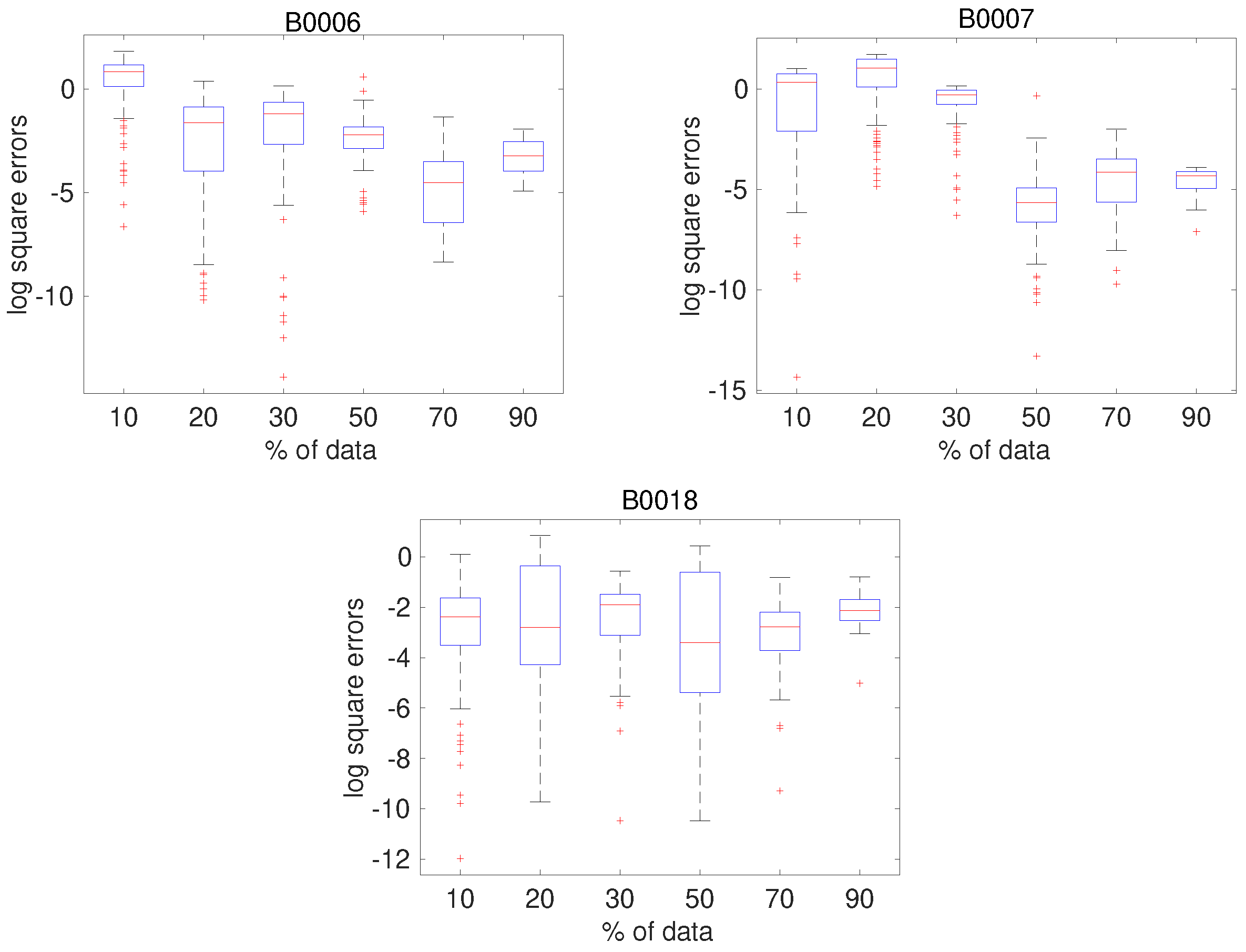
We start with the prediction of the time interval $\delta t(n)$ for the NASA data set, which provides the estimate of the time taken on discharge to reach the threshold voltage. The scalar GP model (9), (10) with kernel (4) and a linear mean function $m(n)={\beta }_0+{\beta }_{1}n$, as outlined Section 2.3, was applied to the data set $\delta t(n)$, $n-1,\dots ,N$ for different numbers of training points. A linear mean function gave the best results over a zero and quadratic. The remaining data points were used for testing. Figure 2 shows boxplots of the square errors on the test points for different percentages of the data points used for training. Results for all three NASA data sets are shown. As can be seen, there is a general trend of declining median error as the percentage of data used for training is increased, except for B0018, for which it remains roughly constant. The important thing to note is that the ranges of error decline for all three data sets.

3.2. Voltage and Temperatures Prediction

Given the interpolated data ${\mathbf{y}}_n{,}_n$, $n=1,\dots ,N$, where ${\mathbf{y}}_n$ is the temperature or voltage and ${}_n$ is the corresponding time sequence, we employed the GP model (5), (6). The latter is given by the prediction for $\delta t(n)$, namely ${\mathbf{t}}_n={(0,\delta t(n),\dots ,199\delta t(n))}^T$, using the data $\{\delta t(n)\}$ corresponding to the same cycle numbers used for training the voltage and temperature model. Again, different kernels were tested and it was found that a mixed SE and linear kernel yielded the best performance overall, with a mixed Matérn and linear kernel also exhibiting good performance. A SE or Matérn kernel alone did not perform well.

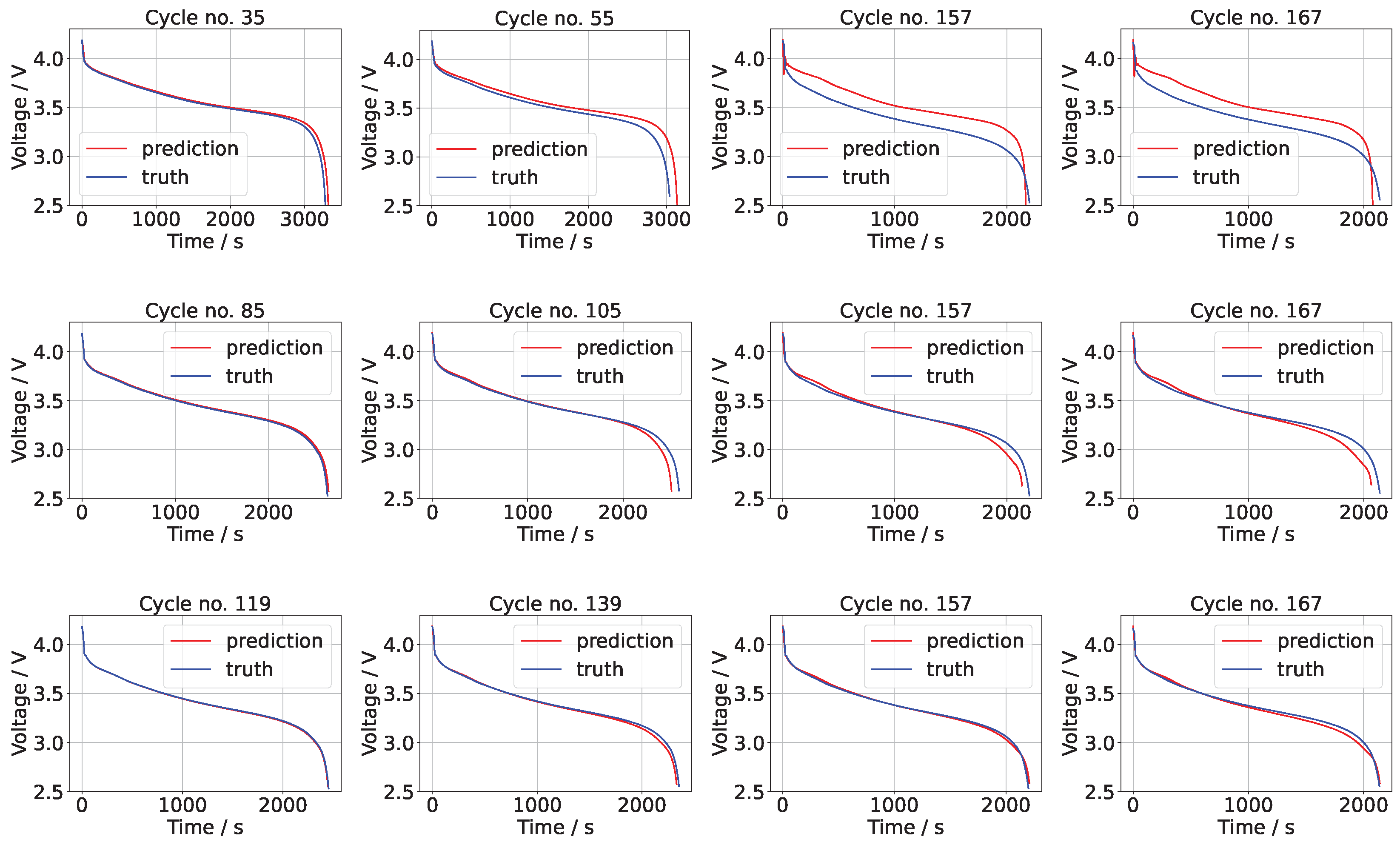
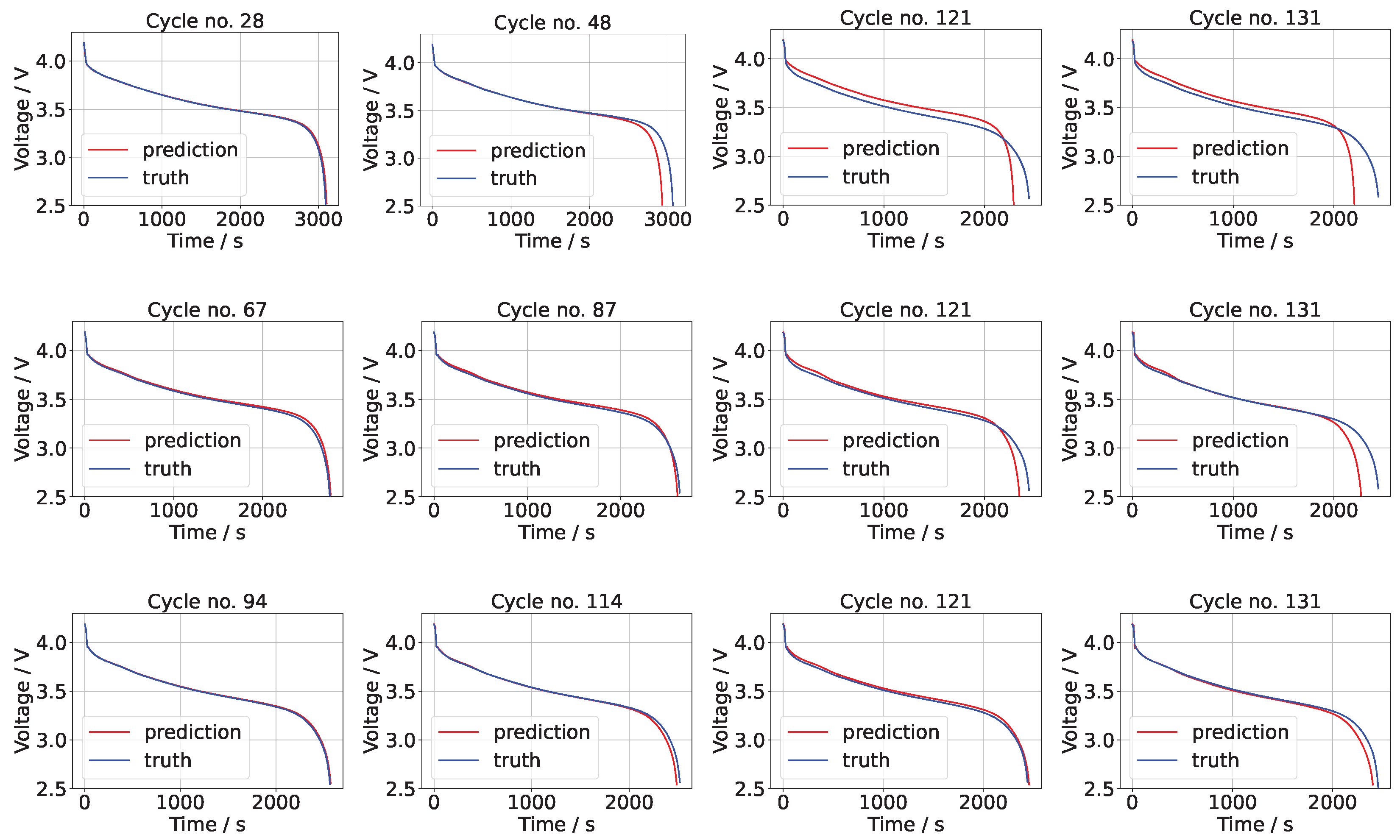
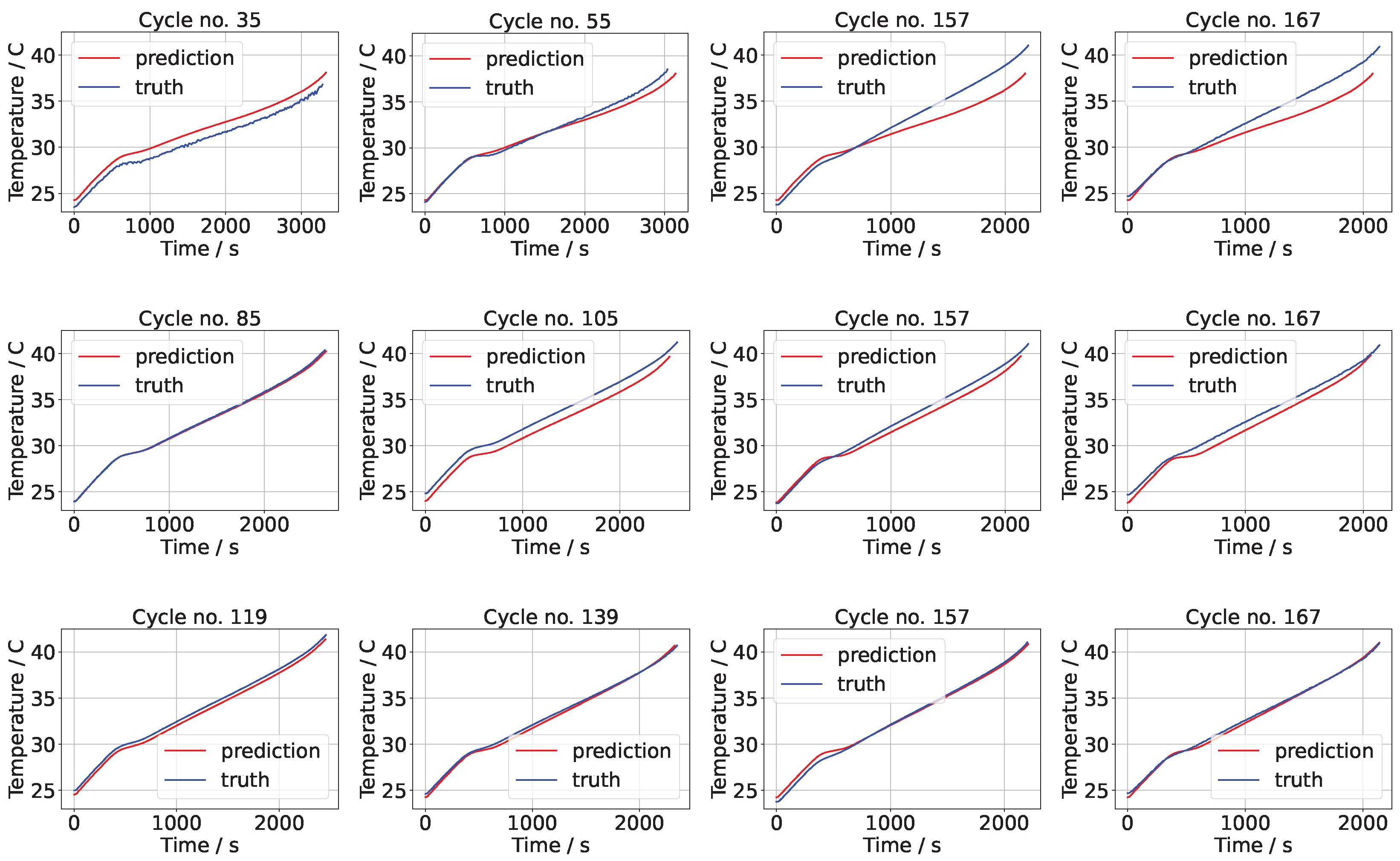
The means of the voltage predictions for the NASA data sets B0006 and B0018 for different numbers of training points are shown in Figure 3 and Figure 4 (the results for B0007 were similar and are omitted to conserve space). In each of these figures it is apparent that the predictions improve with increasing numbers of training points. At low numbers of training points, the initial predictions are accurate but, for increasing cycle numbers, the discrepancy between the prediction and test (truth) grows.

In the case of 20% of the data used for training, the square error (on the prediction of ${\mathbf{y}}_V$ not taking into account the time sequence prediction $\delta t(n)$) on cycle 35 is 0.0317, while the corresponding square error on cycle 167 is 4.859. The RMSE is 1.687 V, which is 0.008435 V per component (out of 200 components). At 50% the results are very accurate, thereafter improving only marginally. The square errors in the case of B0006 are 0.17854, 0.286166 and 0.0780 for 50%, 70%, and 90% on cycle 167, while the RMSE values are 0.2918 V, 0.2438 V, and 0.1145 V for 50%, 70%, and 90%. A similar pattern was found with the other data sets, B0007 and B00018.

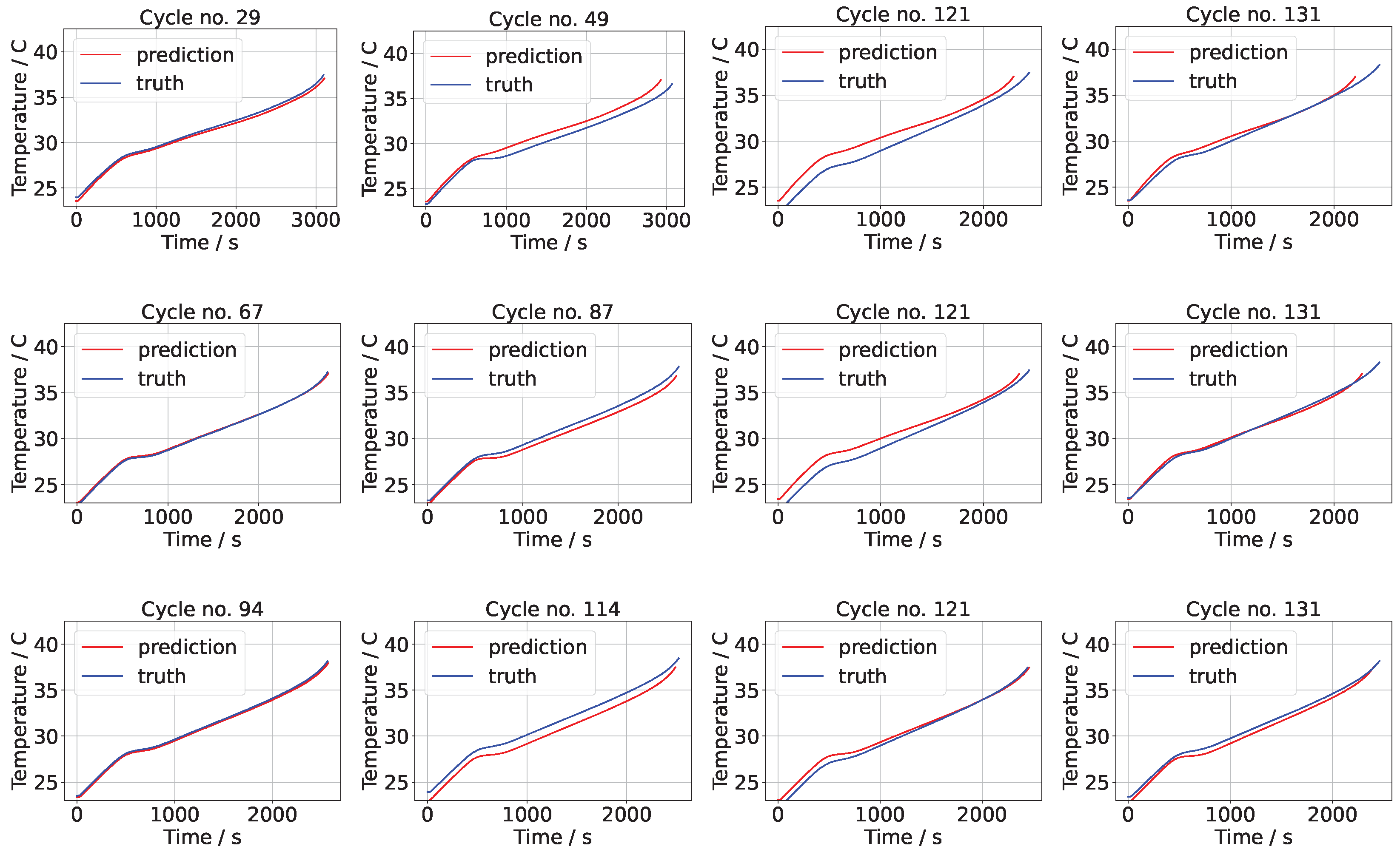
The means of the temperature predictions are shown in Figure 5 and Figure 6 for B0006 and B0007, respectively, exhibiting a similar level of accuracy as the voltage predictions. Again, B0007 was similar and is omitted to conserve space. As with the voltage, the confidence intervals are not shown (only the mean of the posterior GP) since they depend additionally on the variation in the prediction of $\delta t(n)$. Essentially, the voltage and temperature are GP functions of a GP with a particular structure, so capturing the variance in the predictions is not possible. It is noticeable that below 50% of the data for training, the voltage and temperature profiles are not well captured, but the overall trends are predicted well for training point numbers equal to and above 50%.

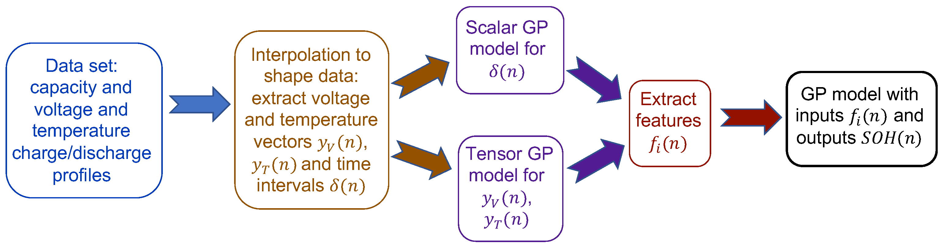
We now use these predictions for multi-step lookahead predictions of the SOH. In order to achieve this, we extract certain features from the predicted voltage and temperature curves. The features we extract are as follows:

(1)

Feature 1. Temperature at the midpoint of the n-th discharge cycle $f_1(n)=T_m(n)$.

(2)

Feature 2. Voltage at the midpoint of the n-th discharge cycle $f_2(n)=V_m(n)$.

(3)

Feature 3. Integral of the n-th voltage discharge curve with respect to time, $f_3(n)=A(n)={\int }_{t}V(n)dt$. This is proportional to the total energy delivered by the battery. A trapezoidal rule was used to estimate the integral.

These features are available from the data set (for training and testing) and can be predicted from the predictive voltage and temperature curves ${\mathbf{y}}_V(n),{\mathbf{y}}_T(n)$ together with the corresponding $\delta t(n)$ for future cycles. Inspection of Figure 1 shows that features 1 and 2 are clearly correlated with SOH. Likewise, the total energy delivered by the battery will decrease as the SOH decreases. We can then use another GP model to learn the mapping from the input $\mathbf{x}(n)={(f_1(n),f_2(n),f_3(n))}^T$ to the SOH, defined as SOH$(n)=C(n)/C(1)$, where $C(n)$ is the capacity at cycle n (available for training and testing from the data set). A schematic of the modeling process is provided in Figure 7.

3.3. SOH Prediction with Predicted Features

The SOH for the NASA data sets is now predicted using the GP model with prior (11) and the equivalent of (9) and (10), with inputs given by the features $\mathbf{x}(n)$, and with outputs SOH$(n)$. Different numbers of training points were employed, including 33%, 50%, and 70% of the total data (168 for B0006/7 and 132 for B0018), with the remainder used for testing. As we would expect, the errors decrease as the number of training points increases. Different mean and kernel functions for the GP model were tested, as discussed below. The RMSE and mean absolute error (MAE) values of the predicted SOH against the test points for all battery datasets are shown in

Table 1. RMSE and MAE for the prediction of the SOH for different training point numbers, % Train (percentage of the total). The results are also shown for a GP model without using the predicted features and for SVR.

B0006
% Train	covariance	mean	RMSE	MAE	GP RMSE	SVR RMSE
33	Matern 3 + 5	linear	0.0260	0.0191	0.0380	0.0420
50	Matern 3 + 5	linear	0.0138	0.0086	0.0229	0.0290
70	Matern 3 + 5	linear	0.0092	0.0067	0.0096	0.0112
B0007
33	2 SE + linear	linear	0.0251	0.0235	0.0621	0.0753
50	2 SE + linear	linear	0.0076	0.0049	0.0156	0.0148
70	2 SE + linear	linear	0.0054	0.0037	0.0084	0.0136
B0018
33	Matern 3 + 5	linear	0.0201	0.0189	0.0409	0.0435
50	Matern 3 + 5	linear	0.0149	0.0126	0.0252	0.0307
70	Matern 3 + 5	linear	0.0151	0.0127	0.0173	0.0221

. The results are shown for the GP method with features $\mathbf{x}(n)$ and for a GP with input n (no features), as well as for support vector regression (SVR) with input n. All codes were executed 10 times and the lowest errors are used in Table 1.

SVR was implemented with both Gaussian and polynomial kernels, including a box search to optimize the hyperparameters. The best performing kernel for SVR was a first-order polynomial, which, nevertheless, yielded the worst performance of all methods overall. We note that Ni et al. [18] also used SVR with a swarm intelligence algorithm to optimize the kernel hyperparameters (similar to the box search). They found a small improvement over a GP method and a large improvement over an LSTM. Given that they used a different data set it is not possible to directly compare their RMSE values with ours. No details were provided for the GP method, so it is not clear how valid is the comparison the authors make, since, as we discuss below, the choice of the kernel and mean function is extremely important.

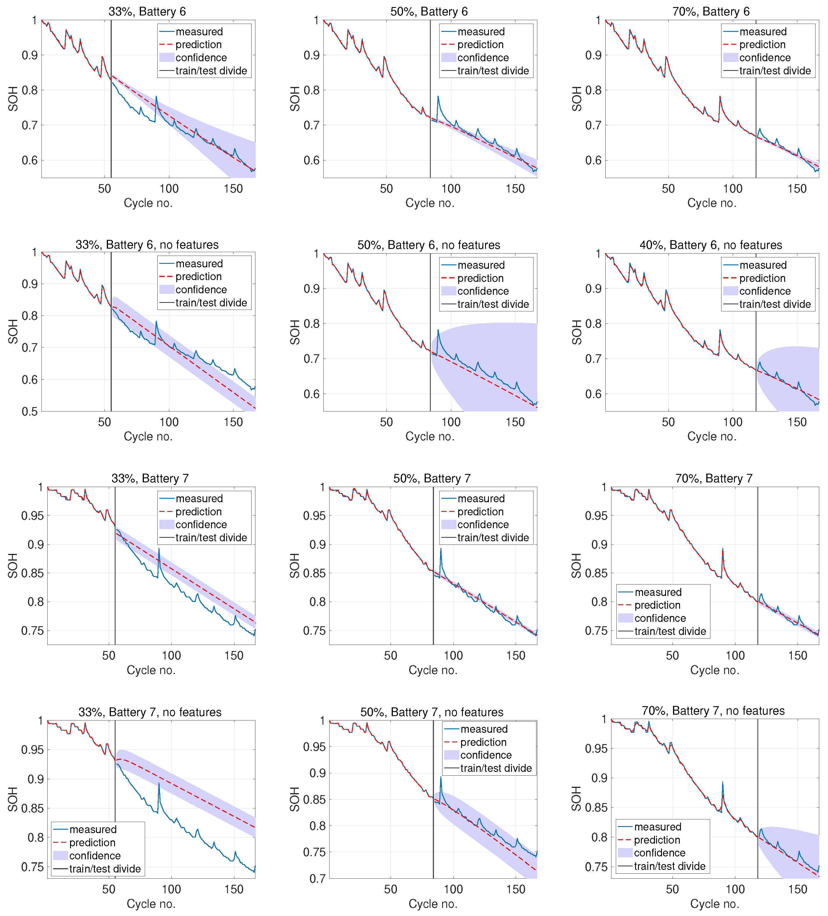
To visualize the quality of the results, in Figure 8 we show the estimated SOH for B0006 and B0007 using the best performing kernel and mean function, for 33%, 50% and 70% of the data used for training. The GP method also provides 95% confidence intervals (shaded regions in the plots), defined as:

$${\mu }_t(n)-1.96{\sigma }_t(n)\le \delta t(n)\le {\mu }_t(n)+1.96{\sigma }_t(n)$$

(14)

in which ${\mu }_t(n)$ and ${\sigma }_t(n)$ are given by (9). We note, however, that these are not precise confidence intervals since the features $\mathbf{x}(n)$ are also predicted means with a predictive variance.

The most important factor was the selection of the covariance function. It was found in this case that the mixed Matérn 3 and 5 of Richardson et al. [16] gave the best results on B0006 and B0018, with the Matérn 1 + linear kernel also performing well. In contrast, a mix of 2 SE kernels of different hyperparameters combined with a linear kernel gave the best performance on B0007; that is:

$$\begin{array}{cc}{\displaystyle k(n,n^{\prime }|\theta )}\hfill & {\displaystyle ={\theta }_{0}exp\left(-\sum _{i=1}^3{\theta }_i{(f_i(n)-f_i(n^{\prime }))}^2\right)+{\theta }_0^{\prime }exp\left(-\sum _{i=1}^3{\theta }_i^{\prime }{(f_i(n)-f_i(n^{\prime }))}^2\right)}\hfill \\ \hfill & {\displaystyle +{\theta }_l\mathbf{x}{(n)}^T\mathbf{x}(n^{\prime })}\hfill \end{array}$$

(15)

with $\mathbf{\theta }={({\theta }_0,\dots ,{\theta }_3,{\theta }_0^{\prime },\dots ,{\theta }_3^{\prime },{\theta }_l)}^T$. Most of the other kernels led to a complete failure of the model.

As also discovered in the pioneering work of Liu et al. [15] and Richardson et al. [16], the mean function $m_s(\mathbf{x}(n))$ plays an important role. A zero or non-zero constant mean function generally provided poor results. In almost all cases, a linear mean function $m_s(\mathbf{x}(n))={\beta }_0+{\beta }_1{f}_1(n)+{\beta }_2{f}_2(n)+{\beta }_3{f}_3(n)$ performed the best, and results are shown only for this mean function in Figure 8 and Table 1.

3.4. Comparison to Recent Methods in the Literature

We compare our results to recently obtained results using the same data set. Yang et al. [27] and Chen et al. [29] discarded some of the data points as outliers. We did not discard any values, although such an approach would certainly have improved the accuracy of our results to an extent, depending upon how many values were discarded.

For the case of 84 and 118 training points from B0006, we were able to obtain mean absolute errors of 0.0086 and 0.0067. The deep GP approach of Tagade et al. [33] using features as inputs (Figure 3 of their paper) obtained MAE values of ca. 0.009 and 0.008 (divided by the nominal capacity of 2 Ah) for 100 and 120 training points. A deep GP is significantly more expensive than a standard GP, since the posterior is not tractable and therefore requires sampling, while training is via expensive approximate Baye’s (e.g., variational) or Markov Chain Monte-Carlo sampling methods.

Yang et al. [27] achieved RMSE values of 0.0149 and 0.0078 for B0006 and B0007 at 80 training points (the only case considered), which is roughly 50% of the data (Table 4 in their paper), again using features as inputs. This compares with 0.0138 and 0.0076 in Table 1, respectively, despite the fact that we did not remove any data points. Chen et al. [29] discarded 60 of the 168 data points for B0006 and 36 of the 132 data points for B0018, without specifying which were removed. Using their LSTM model with 4 features they were, therefore, able to obtain much lower RMSE values between 0.0025 and 0.0012 for B0006 and B0018, depending on the proportion of data used for training.

The aforementioned methods, as well as the capacity models in [32,34], however, can only predict one cycle, since the features pertaining to future cycles are unavailable. This means that any errors calculated on a test set of more than one point (including all of those quoted above) are misleading; the calculation of such an error could never be realized in practice. We note that Zhao et al. [41] used features extracted from a capacity sequence based on a random vector functional-link neural network. These features were fed as inputs into an LSTM for predicting the capacity (or SOH). This method is therefore capable of recursive application because the features are not exogenous inputs as in the other cases. The RMSE value for B0006 was 0.0087 for 25% of the training data. However, 40 unspecified data points were discarded, which again makes the comparison invalid. It is always possible to lower the RMSE considerably by selectively choosing points to discard, e.g., those exhibiting the highest errors.

Incorporating features that are not predicted (as in our model) for K-step lookahead could be possible with a direct time series strategy, in which K different models $f_k$ are developed based on different embeddings, with $f_k$ predicting the SOH k cycles ahead. All models are required for the full sequence of $n+1,\dots ,n+K$ predictions. Alternatively, a sequence to sequence approach can be used in which specified sequences of inputs/features are used to predict sequences of future capacity values with some specified length. How such strategies compare to approaches that do not use features or to recursive methods is not known. There is a plethora of choices, in terms of the features used, embeddings, and machine learning methods. These are the subject of a forthcoming paper on linear and nonlinear autoregressive approaches, including deep learning, GP models, and classical state-space approaches.

3.5. Assessing the Effect of Noise

It can be seen in Figure 1 that the capacity does not change in a monotonic fashion, with small fluctuations about an overall decreasing trend (Figure 1). This is possibly due in part to a so-called regeneration phenomenon, in which the capacity rises temporarily, before returning within a few cycles to the overall trajectory. It is clear, however, that the fluctuations have a random component, with at least some part due to measurement and possibly human error.

For experimental time series, $u(1),\dots ,u(N)$, there are several empirical measures of irregularity or randomness, such as the approximate entropy and the sample entropy [42]. They essentially measure the probability that patterns of observations arranged as vectors $\mathbf{w}(i)=(u(i),u(i+1),\dots ,u(i+E-1))$ are proceeded by similar patterns of observations. Here, E is the embedding size. In the case of the approximate entropy, the metric for measuring the distance between two patterns is given by the max norm $d(\mathbf{w}(i),\mathbf{w}(j))={\parallel \mathbf{w}(i)-\mathbf{w}(j)\parallel }_{\infty }={max}_{k=1,\dots ,E}|u(i+k-1)-u(j+k-1)|$. The number of patterns that are similar to a given pattern $\mathbf{w}(i)$ is then counted as follows:

$$C_i^E(r)=\frac{\mathrm{number}\mathrm{of} j\le N-E+1 \mathrm{such} \mathrm{that}d(\mathbf{w}(i),\mathbf{w}(j))\le r}{N-E+1}$$

(16)

by defining similarity as falling within a ball of the radius or filter size r. Defining:

$${\psi }^E(r)=\frac{1}{N-E+1}\sum _{i=1}^{N-E+1}log{C}_i^E(r)$$

(17)

the approximate entropy is calculated as $AE(E,r,N)={\psi }^E(r)-{\psi }^{E+1}(r)$. Sample entropy is calculated in a different but related manner. Low values of approximate and sample entropy (close to zero) suggest that a system has a persistent, repetitive, and predictive pattern, while high values suggest a degree of independence between data points, inferring randomness and few repeated patterns.

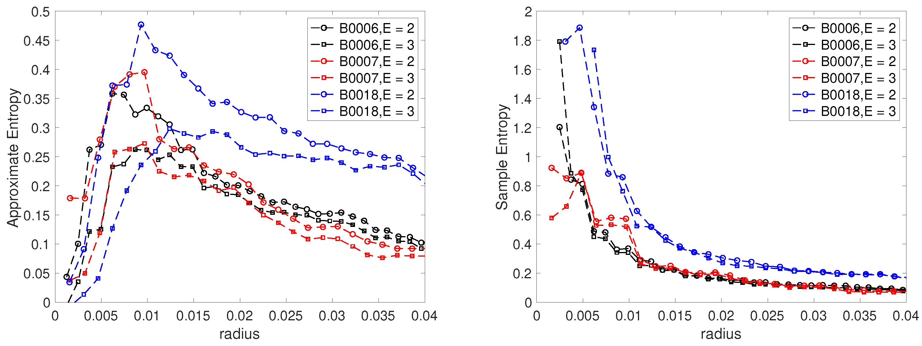
For each battery, the approximate and sample entropies are shown in Figure 9. The values are shown for $E=2$ and $E=3$ (those usually recommended) and varying radius r. The radius is normally chosen as $r=c{\sigma }^2$, in which ${\sigma }^2$ is the sample variance of the time series and c is a constant, usually in the range $c\in (0.1,0.25)$. In Figure 9, we show values of the entropies for $c\in (0.01,0.25)$ using the largest variance across the data sets. All three batteries, especially B0018, exhibit large values, suggesting a high degree of randomness (noise).

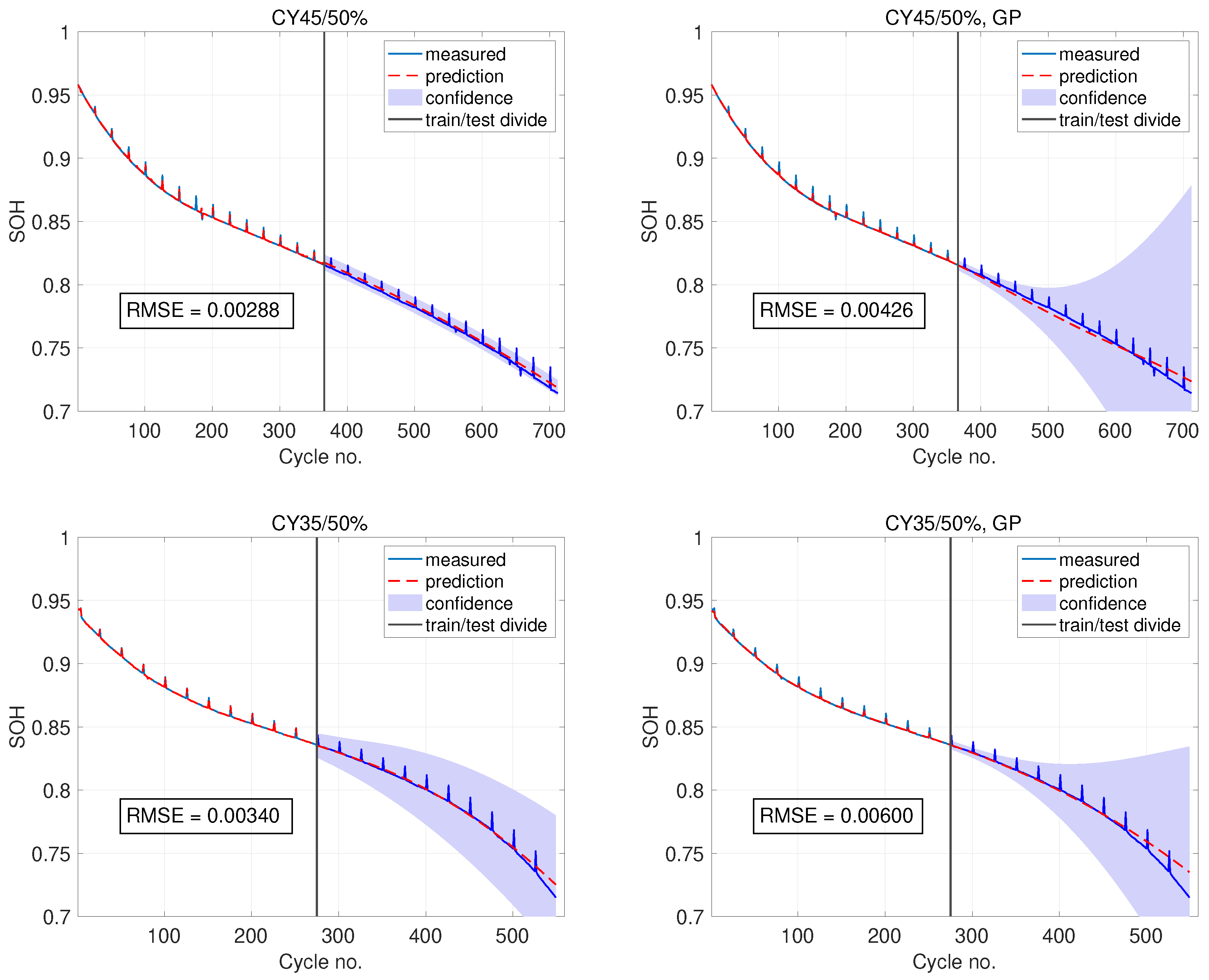
To assess the performance of our method in cases with less noise, we used the data set in [37]. We show results for 2 NCA batteries cycled at 45C and 35C, with a charge current of 1.75A and a discharge current of 3.5A. They are labeled CY45 and CY35, respectively. Several batteries were cycled, and we show the results for those labeled #1. The results for the other batteries were similar. Both the sample and approximate entropies of these data sets are less than 0.04 for $c=0.25$, and peak at around $c=0.005$, with values below 0.18. This indicates that the level of noise in both data sets is low.

The prediction of the SOH using 50% of the data (366 cycles and 278 cycles, respectively) is shown in Figure 10, for our method and for a GP using the cycle number as input. For the GP with input n, a SE kernel with a zero mean function gave the best results. In this case, only features 2 and 3 are used, since temperature data was not available. When features were used as inputs, the best performance was with the mixed kernel (15), with a linear mean function. The experimental SOH curves exhibit oscillations, indicative of regeneration. In this case, however, the fluctuations occur at regularly spaced intervals in time and have a small amplitude.

The RMSE and MAE values are shown in this figure for both cases. It can be seen that the inclusion of features again enhances the predictions. What is also noticeable (as with the NASA data sets) is that the confidence intervals are less broad compared to the standard GP approach, which predicts with low confidence. However, the confidence intervals for the case with features are less precise, as previously mentioned. These results show that noise is an important factor. With only 50% of the training data, a GP model without features can predict with an error one order of magnitude lower than on the NASA data set. With predictive features, the error can be further lowered to provide highly accurate predictions.

3.6. Computational Times

The execution of the codes is extremely rapid. We quote the times for the battery B0007 data set, averaged over 5 runs. All calculations were performed on a Macbook Pro 2.3 GHz, 8-Core i9 with 64 GB DDR4 RAM. The codes were implemented in Python for the voltage and temperature predictions and in MATLAB for the predictions of the time interval and SOH, as well as the feature extraction.

The interpolation procedure during preprocessing took, on average, 0.118 s. The estimation of the time intervals using (5), (6) for B0007 took an average of 0.767 s using 50% of the training data, while for 70% of the data the average time was 0.865s. For the estimation of the voltage and temperature curves for B0007 using the GP model (5), (6), the time taken was 0.499 s for 50% of the data, while the corresponding time for 70% of the data was 0.577 s. Extracting the predictive features for B0007 in the case of 50% of the training data took 0.112 s, and 0.130 s in the case of 70%. SOH predictions using the GP prior (11) and the equivalent of (9) and (10) then took 1.092 for 50% of the data and 1.222 s for 70% of the data. Thus, for 70% of the data, the total time is ca. 2.92 s, which can be lowered by running the predictions for the time interval and voltage/temperature curves in parallel. These times are much shorter than would be required for typical deep learning architectures. We present such a comparison in a future paper.

4. Summary and Conclusions

The development of algorithms for predicting the state of health of batteries is critical for electric vehicle applications. Data-driven approaches often use features to enhance predictions. These features are extracted from various data available from a BMS, including voltage, current, and temperature measurements. However, they cannot be used directly to develop recursive or direct supervised machine learning algorithms that are capable of early predictions of the EOL.

To overcome this limitation, we developed a novel approach in which features are predicted for future cycles, enabling predictions of the SOH for an arbitrary number of cycles ahead, and, therefore, predictions for the EOL. We showed that these predicted features enhance the accuracy of the SOH predictions. We also investigated the effects of noise and showed that with low-noise data, very accurate predictions can be realized. The approach we develop is not specific to a Gaussian process model, although such models are known to be very accurate and can provide uncertainty bounds. In future work, we intend to investigate the use of joint learning of the voltage, temperature, time interval, and SOH, which could further enhance predictions.