Abstract
The P-S-N curve is a vital tool for dealing with fatigue life analysis, and its fitting under the condition of small samples is always concerned. In the view that the three parameters of the P-S-N curve equation can better describe the relationship between stress and fatigue life in the middle- and long-life range, this paper proposes an improved maximum likelihood method (IMLM). The backward statistical inference method (BSIM) recently proposed has been proven to be a good solution to the two-parameter P-S-N curve fitting problem under the condition of small samples. Because of the addition of an unknown parameter, the problem exists in the search for the optimal solution to the three-parameter P-S-N curve fitting. Considering that the maximum likelihood estimation is a commonly used P-S-N curve fitting method, and the rationality of its search for the optimal solution is better than that of BSIM, a new method combining BSIM and the maximum likelihood estimation is proposed. In addition to the BSIM advantage of expanding the sample information, the IMLM also has the advantage of more reasonable optimal solution search criteria, which improves the disadvantage of BSIM in parameter search. Finally, through the simulation tests and the fatigue test, the P-S-N curve fitting was carried out by using the traditional group method (GM), BSIM, and IMLM, respectively. The results show that the IMLM has the highest fitting accuracy. A test arrangement method is proposed accordingly.
1. Introduction
In the design of key engineering equipment, anti-fatigue design is one of the most important considerations [1,2] because the critical components of such equipment are often subjected to long-term variable loads. In the field of fatigue life prediction, the P-S-N (probability of survival-stress/strain number of cycles) curve of material or part is an important tool to describe the relationship among the survival rate, stress, and fatigue life [3,4].
In practical engineering, due to the limitation of time and cost, the large-scale fatigue test is usually not feasible. In many cases, data from fatigue tests are limited, or there are only a few samples. Under such circumstances, many studies have focused on how to minimize the sample size and shorten the experimental time [5,6,7,8]. However, how to make better statistical analysis of experimental data and obtain more accurate P-S-N curve estimation with limited data has always been a concern of scholars [9,10,11,12].
The three-parameter P-S-N curve is a common form that can better describe the fatigue behavior of materials and parts. Because, in metal materials, the P-S-N curve in the middle- and long-life range is no longer linear in the logarithmic coordinate system [13]. There have been numerous types of fitting techniques developed and widely used in advanced statistical analysis, including the maximum likelihood method (MLM) [14,15,16,17,18], the group method (GM) [19,20,21,22,23,24,25,26,27], and the backward statistical inference method (BSIM) [28,29,30,31].
For MLM, the concept of likelihood was first put forward by Lambert [14] and then was used by the ASTM standard [15] to fit the two-parameter P-S-N curve in detail. Then, MLM was used for three-parameter P-S-N curve fitting. As mentioned in references [16,17], the advantage of MLM is that it greatly reduces the time cost and the number of samples needed to solve the fitting parameters accurately. In the case of a large number of samples at a certain stress level, Jing [18] used the MLM to fit P-S-N curves, reducing the number of unknown parameters.
The GM [19,20] was first applied to two-parameter P-S-N curve fitting [21], assuming that the standard deviation of life is independent of stress [22,23]. At each test stress level, the GM evaluates points under a given probability (and confidence limit) and then considers these points for P-S-N regression. The GM can only obtain accurate P-S-N results when the sample size is large enough [24,25,26]. Fu [27] obtained the fatigue limit parameters through testing and then used the GM to fit the P-S-N curves.
The BSIM was proposed by Xie [1,28] based on the fatigue life percentile consistency. Li [29] determined the interval and method of parameter search. However, the assumption that a linear relation between logarithmic life standard deviation and stress is inconsistent with the S-N equation adopted. Tan [30] revised the assumption and determined the needed number of specimens in the test of P-S-N curves under a given relative error. Bai [31] assumed that the coefficients of logarithmic fatigue life variation at different stress levels are equal and integrated all lives by the BSIM to obtain the life distribution parameter.
A concurrent probability method has recently been proposed to estimate the P-S-N curves, which are based on mid-long life test data and fatigue limits [32]. For fatigue reliability analysis, the survival analysis described the fatigue failure process to produce a set of flexible and accurate P-S-N curves [33]. The fitting methods of the P-S-N equation were given using Bayesian methods [34,35]. Because of the need to deal with the selection of prior distribution, these methods are suitable for the case of known information prior. If the available training fatigue database is large enough, a neural network method [36] for composite materials can be used to describe the scatters of S-N curves. The disadvantage is the need to select the appropriate input parameters and network structure. A recursive neural network was applied to composite materials [37] to overcome the shortcoming of network structure selection. However, when the sample size is small, it is difficult to get reasonable three-parameter P-S-N curves due to unreasonable assumptions and low accuracy.
How to determine the minimum sample size for fatigue tests is a problem of concern. To determine the sample size, Gope P C [38,39] studied sample size estimation methods for the lognormal distribution and Weibull distribution. Efron B [40] proposed an enhanced sample statistics method with a certain confidence level. Fu H [41] proposed a unilateral tolerance factor through statistical inference and gave the relative error at the unilateral confidence lower limit.
In this paper, the principle of sample information aggregation is introduced into the three-parameter P-S-N curve fitting first, and then the BSIM method is proposed. The three-parameter P-S-N curve fitting process of GM is introduced secondly. Then, an improved maximum likelihood method (IMLM) is proposed, which combines the principle of sample information aggregation with the MLM. In order to verify the effectiveness of the three methods, the P-S-N curve fitting is carried out based on simulation data and experimental data. Finally, the determination of the minimum number of specimens in P-S-N testing was proposed considering the given relative error and confidence.
2. Improved Methods
2.1. BSIM
Based on the rule of consistency of failure trace [42], the BSIM converts the lives under different stresses to expand the application of sample information. Now, this method is extended to the fitting of the three-parameter P-S-N curve.
Supposing the fatigue life N follows a lognormal distribution, survival rate p can be expressed as follows
where np is the fatigue life n associated with 1p%, s and μ are the standard deviation and mean value of log(N), respectively, and Φ(•) is the standard normal distribution function. If under stress σj and the survival rate of sample i is p, then under the stress level σk, its survival rate is still p. This means that a sample that is weak (strong) at one stress level will be weak (strong) at another stress level. The failure track followed by the specimen is the current P-S-N curve, as shown in Figure 1.
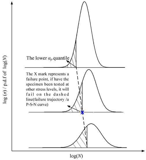
Figure 1.
Fatigue life percentile consistency principle.
So, it can be given as
where nji is the fatigue life of sample i at σj, transforming it into
According to Equation (1), fatigue lives from other stresses and can be converted to one stress, as shown in Figure 2. Thus, the sample information can be extended. To achieve the goal, we need to determine the relation between μ, s, and σ, respectively.
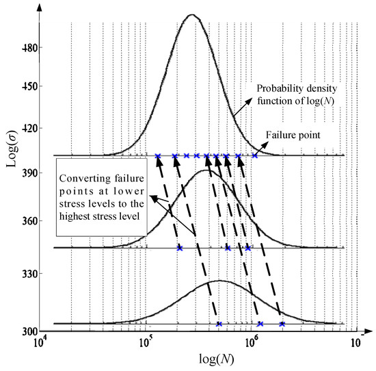
Figure 2.
Fatigue life conversion.
The equation of the three-parameters P-S-N curve is [43]
where mp, Cp, and σ0p are material parameters corresponding to p. We take the logarithm on two sides:
So, the median S-N curve is
The relationship between μ and σ is obtained. Next, we need to determine the relationship between s and σ. Deforming Equation (1) gives:
Combining Equations (5)–(7) gives
When p = 0.99, s is demonstrated as
The relationship between s and σ is obtained. The relationship between standard deviations at different stress levels is needed for the conversion. The relation between sk and sj is derived as
From Equation (10), sk is determined by four unknown parameters, σ0,50, σ0,99, m99, and sj. Using logarithmic fatigue lives at all levels of stress, m50 can be easily calculated. Obviously, after the life standard deviation is determined for certain stress (for example, the highest stress, s1), the relationship of life standard deviation–stress can be determined by σ0,50, σ0,99, and m99.
Such transformation is equivalent to changing the life formation process (changing the stress) of the same sample and obtaining fatigue life data under different stresses. This achieves the purpose of enlarging the sample size.
The judgment of search termination is that the relative error of logarithmic life standard deviation of the target stress level before and after life data conversion reaches a minimum. So, one can use Equations (3)and (10) to fit P-S-N curves. The parameters to be searched and determined include σ0,50, σ0,99, and m99. Obviously, the search range for σ0,50 and σ0,99 is [0, σmin]. If the number of samples corresponding to the target stress level is less than 6, the s of the target stress level should also be searched [29]. The overall steps are as follows.
(1) Take the mean of the logarithmic lives at σj,
where qj is the sample size at σj.
(2) Search for σ0,50 in the set [0, σmin], and the step size is 0.1 MPa. For each σ0,50 to fit the relationship between the sample mean and stress by the least squares method, thus acquiring the 50%-S-N equation as
(3) Then, determine the value range of s1 (parent standard deviation at the highest stress σ1). When there is only one sample at σ1, the value range of s1 can refer to materials with similar properties. When samples are larger than one and smaller than six at σ1, the sample standard deviation is calculated by
Thus, the search region of s1 can be [0.1s1′, 10s1′]. Otherwise, s1′ is directly determined by Equation (11).
(4) As for each s1, search for σ0,99 in the set [0, σmin] and m99 in the set [0, 10m50]. Given each parameter set, s1, σ0,99, and m99, based on Equations (3) and (10), it is possible to convert fatigue lives at other stress levels into fatigue lives at level σ1.
(5) As a result of the conversion, s1′ at σ1 can be recalculated by using the whole samples.
(6) Determine the optimal parameter set, s1, σ0,99 and m99, which makes the relative error, |s1 − s1′|/s1, the smallest. Then, the at each stress level can be finally obtained by Equation (10).
(7) The logarithmic life at p can be calculated by log(np) = , where h is the one-side tolerance factor associated with three parameters: p, confidence γ, and freedom degree T-1 (T represents the total number of samples).
and
where tγ is the t-distribution’s γ percentile, and β is the correction coefficient of standard deviation.
Finally, the P-S-N equation can be obtained by fitting the relation between log(np) and stress with the least squares method.
2.2. GM
This is a traditional P-S-N curve fitting method, which directly searches for the three unknown parameters of the P-S-N curve equation by calculating the standard deviation and the mean value of logarithmic life at each stress level. The overall steps are as follows:
- (1)
- Calculate the sample mean and standard deviation of the logarithmic lives at all stresses, respectively;
- (2)
- Search σ0,50 in the region [0, σmin] and set the step size as 0.1 MPa. For each σ0,50, the median S-N equation, = log(C50) − m50log(σ − σ0,50), is derived by fitting all sample means by the least squares method;
- (3)
- Search σ0,99 in the region [0, σmin] and set the step size as 0.1 MPa. For each σ0,99, the logarithmic life at p can be calculated by log(np) = . Finally, the P-S-N equation can be obtained by fitting the relation between log(np) and stress with the least squares method.
2.3. IMLM
In the BSIM, the judgment of search termination is that the relative error of logarithmic life standard deviation of target stress level before and after life data conversion reaches a minimum. This criterion is not rigorous, so multiple sets of solutions may occur. The MLM can solve this problem. By applying the principle of sample aggregation to the maximum likelihood estimation, the estimation accuracy can be improved by increasing the sample information.
The stress level σr with no less than six samples is selected as the reference stress level, and the sample’s mean, μr, and standard deviation, sr, are obtained. If there is no stress with large samples, the highest stress level is selected as σr, and its corresponding life standard deviation is treated as an unknown parameter. The logarithmic life standard deviation is expressed as
where σ0,50 and m50 are determined by the same method of BSIM in Step (1) and Step (2). According to the assumption that the fatigue life follows the lognormal distribution, the probability density function of life N at stress i is
Then, according to Equation (3), all life samples were converted to other stress levels to obtain the extended life samples. Considering life samples at all stress levels a, the maximum likelihood function L is established as
We define F as
When F achieves a minimum, the maximum likelihood function L achieves a maximum. Therefore, the search procedure of this method is the same as that of BSIM except that the search end criterion in the 6th step, which is that F achieves the minimum value. The flow chart is shown in Figure 3.
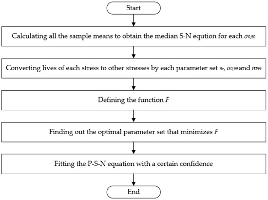
Figure 3.
The flow chart of the IMLM.
This method enlarges the life sample size by a times so that the search precision of the optimal solution is improved. The overall steps are as follows.
(1) Take the mean of the logarithmic lives by Equation (11).
(2) Search for σ0,50 in the set [0, σmin], and the step size is 0.1 MPa. For each σ0,50 to fit the relation between the sample mean and stress by the least squares method, thus acquiring the 50%-S-N equation by Equation (12).
(3) The stress level σr with no less than six samples is selected as the reference stress level. If there is no stress with large samples, then the highest stress level is selected as σr. Then, determine the value range of sr (parent standard deviation at the reference stress σr). When there is only one sample at σr, the value range of sr can refer to materials with similar properties. When samples are larger than one and smaller than six at σr, the sample standard deviation is calculated by
where qr is the sample size at σr, µr′ is the mean of the logarithmic lives at σr, nr,i is the ith life at σr. Thus, the search region of sr can be [0.1sr′, 10sr′]. Otherwise, sr′ is directly determined by Equation (20).
(4) As to each sr, search for σ0,99 in the set [0, σmin] and m99 in the set [0, 10m50]. Given each parameter set, sr, σ0,99, and m99, based on Equation (3) and Equation (16), it is possible to convert fatigue lives at other stress levels into fatigue lives at level σr.
(5) As a result of the conversion, the logarithmic life standard deviation can be recalculated by Equation (16).
(6) Determine the optimal parameter set, sr, σ0,99, and m99, which makes the F the smallest by Equation (19). Then the at each stress level can be finally obtained by Equation (16).
(7) The logarithmic life at p can be calculated by log(np) =. Finally, the P-S-N equation can be obtained by fitting the relation between log(np) and stress with the least squares method.
3. Validations
3.1. Simulation Comparisons
In this part, random life samples are generated using the known P-S-N equations. The above three methods are used to derive the P-S-N equations, and the relative errors of results are compared with the known P-S-N equations to find out the best method.
- (1)
- The first simulation test.
The known 50%- and 99%-S-N equations used by the first set of simulations are and . Fifteen stress levels are set, and one random life sample is generated for each stress, as shown in Table 1. Since the GM could not obtain the life standard deviation under this condition, only BSIM and IMLM were used for comparative verification. The results are shown in Figure 4.

Table 1.
Simulated samples generated from the known P-S-N equations.
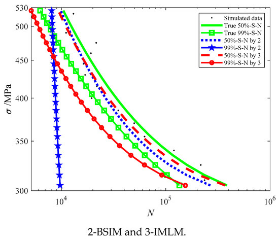
Figure 4.
The fitting results of the first simulation set by BSIM and IMLM.
Obviously, the P-S-N curves obtained by IMLM are closer to the original curves in Figure 4. Compared with the known P-S-N equations, the average relative errors of 50%-S-N obtained by BSIM and IMLM are 19.29% and 13.88%, respectively. Compared with the known P-S-N equations, the average relative errors of 99%S-N obtained by BSIM and IMLM are 43.39% and 23.54%, respectively.
- (2)
- The second simulation test.
The given P-S-N equations remain unchanged. Five stress levels are set, and three life samples are randomly generated for each stress level, as shown in Table 2.
Table 2.
Simulated samples generated from the known P-S-N equations.
Three methods are used for comparison and verification, and the results are shown in Figure 5. It is clear that the P-S-N curves obtained by GM deviate too much from the known P-S-N curves. Compared with the known P-S-N equations, the average relative errors of 50%S-N obtained by GM, BSIM, and IMLM are 23.71%, 12.32%, and 9.6%, respectively. Compared with the known P-S-N equations, the average relative errors of 99%-S-N obtained by GM, BSIM, and IMLM are 46.25%, 29.2%, and 12.19%, respectively. The IMLM is comparatively more effective.
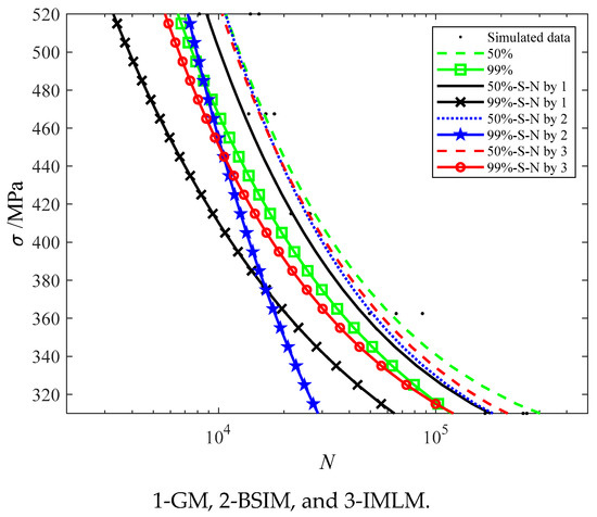
Figure 5.
The fitting results of the second simulation by GM, BSIM, and IMLM.
3.2. Experimental Comparisons
Finally, the comparison and verification of the three methods are carried out by the fatigue test data, and five stress levels are adopted. The fatigue test specimen [43] and data are shown in Figure 6 and Table 3. The stress ratio is −1. The loading frequency is 10 Hz.
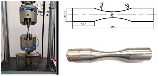
Figure 6.
The 20MnTiB fatigue specimen and test equipment (mm).
Table 3.
Experimental results by tensile and compression testing.
From Figure 7, it is clear that the GM deviates too much. The life standard deviation obtained by BSIM and GM does not increase with the decrease in stress, so it is not consistent with the actual situation. A large number of tests show that the standard deviation of life increases with a decrease in stress [28]. Therefore, the BSIM and GM fitting result is unreasonable. The life standard deviation of IMLM increases with the decrease in stress, which is consistent with the actual situation. The BSIM is superior to the GM because it expands the sample information. The IMLM is superior to BSIM because it optimizes the search criteria. The IMLM not only enlarges the sample information but also has better boundary conditions.
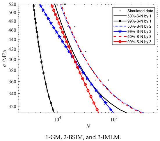
Figure 7.
The fitting results of the fatigue test by GM, BSIM, and IMLM.
4. Arrangement of Specimens in a P-S-N Test
In the fatigue test, the minimum sample should be used to obtain the P-S-N curve with the given relative error. Usually, the fatigue test is carried out first, and then the fitting is carried out rather than adjusting the sample arrangement with the experimental data. This results in waste or insufficiency of specimens under certain stresses. This chapter presents a method to adjust the arrangement of the next specimen with the result of each sample. The results of this method are compared with those of traditional test methods by simulation.
First, determine the minimum sample size, nmin, required for each stress [41] by Equation (21):
where δ denotes the unilateral relative error between the confidence lower limit µ′ + hs′ and the parent truth value µ + αps, µ′ is the sample mean, and s′ is the sample standard deviation. nmin at all stress levels should be calculated at all times when the test is performed under the given conditions of δ, αp, and γ.
To determine µ′ and s′, a test should be carried out at each stress level. Then calculate the two parameters according to the steps in Section 2.3. Then, nmin is calculated, and the fatigue test is conducted again on the stress where the number of specimens is the largest difference from nmin. The above step is repeated until the number of test pieces is not less than the corresponding nmin for each stress.
By the conventional method, at least two specimens should be tested at each stress to obtain sample standard deviation(see Section 2.2). Then, nmin is calculated for each stress, and another test specimen is added to the stress where the number of test specimens differs the most from nmin. The above step is repeated until the number of test pieces is not less than the corresponding nmin for each stress.
To compare the two test schemes, use the given P-S-N curves to generate life samples to simulate fatigue tests randomly. The adopted 50%-S-N equation is , and the 99%-S-N equation is .
Five stress levels were evenly selected between 310 MPa and 520 MPa to cover the high cycle fatigue life range. With γ = 90% and δ = 0.01, the objective of the experiment is to obtain a 99%-S-N curve using the minimum specimen. As shown in Table 4, all samples are the results of the conventional method; only the bold samples are the results of the method in this paper.
Table 4.
Simulated test results of two methods.
In Figure 8, The fitting results of 99%-S-N curve and the corresponding true 99%-S-N curve are shown. By comparing this method with the true 99%-S-N curve, the 99%-S-N curve with an average relative error of 1.3% is obtained by using only 12 samples (2-2-3-3). Thirty-six samples are used by the conventional method (5-6-7-8-10), and the mean relative error is 1.4%. Under the same conditions, the minimum sample required by the traditional method is three times that of the proposed method.
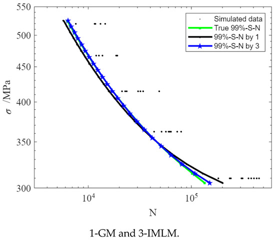
Figure 8.
Sample arrangement and 99%-S-N curve obtained by two methods.
5. Conclusions
This paper compares the advantages and disadvantages of GM, BSIM, and IMLM, aiming at the three-parameter P-S-N curve fitting in the case of small samples, and draws the following conclusions:
- (1)
- Through the simulation test, the comparison with the original P-S-N curve proves that IMLM has the best fitting effect among the three methods, followed by BSIM. The GM method has an application limitation; it cannot be used in a situation where the stress level has only one life sample;
- (2)
- The fatigue test shows that, among the three methods, IMLM can reflect the characteristic of life dispersion increasing with the decrease of stress, and the fitting result is reasonable;
- (3)
- The IMLM combining the advantages of BSIM and the maximum likelihood estimation has high-fitting accuracy. The advantage of IMLM is that it expands the sample information, so it improves the disadvantage caused by the small sample size. At the same time, it has a reasonable optimal solution search criterion, which makes up for the deficiency of the BSIM method;
- (4)
- According to the test scheme proposed according to the IMLM, a large number of samples are saved compared with the traditional method under the same precision requirement.
In this paper, there are still deficiencies in the search for the best parameters, and the search speed will be improved next. On the basis of this study, we will try to study a small-sample P-S-N curve fitting under the Weibull distribution in the future.
Author Contributions
Conceptualization, X.T. and Q.L.; methodology, X.T.; software, X.T.; validation, X.T., G.W.; formal analysis, K.X.; investigation, X.T.; resources, X.T.; data curation, X.T.; writing—original draft preparation, X.T.; writing—review and editing, X.T.; visualization, X.T.; supervision, X.T.; project administration, X.T.; funding acquisition, X.T. All authors have read and agreed to the published version of the manuscript.
Funding
This research was funded by [the High-level Personnel Scientific Research Start-up Fund Project of Weifang University of Science and Technology] grant number [KJRC2019011]. And The APC was funded by [the High-level Personnel Scientific Research Start-up Fund Project of Weifang University of Science and Technology].
Data Availability Statement
The data presented in this study are available in this article.
Conflicts of Interest
The authors declare no conflict of interest.
References
- Amiri, N.; Farrahi, G.; Kashyzadeh, K.R.; Chizari, M. Applications of ultrasonic testing and machine learning methods to predict the static & fatigue behavior of spot-welded joints. J. Manuf. Process. 2020, 52, 26–34. [Google Scholar]
- Jouini, N.; Revel, P.; Thoquenne, G. Influence of surface integrity on fatigue life of bearing rings finished by precision hard turning and grinding. J. Manuf. Process. 2020, 57, 444–451. [Google Scholar] [CrossRef]
- Tan, X.; Xie, L. Fatigue reliability evaluation method of a gear transmission system under variable amplitude loading. IEEE Trans. Reliab. 2018, 68, 599–608. [Google Scholar] [CrossRef]
- Hoole, J.; Sartor, P.; Booker, J.; Cooper, J.; Gogouvitis, X.V.; Schmidt, R.K. Systematic statistical characterisation of stress-life datasets using 3-Parameter distributions. Int. J. Fatigue 2019, 129, 105216. [Google Scholar] [CrossRef]
- Zheng, X.L.; Wei, J.F. On the prediction of P-S-N curves of 45 steel notched elements and probability distribution of fatigue life under variable amplitude loading from tensile properties. Int. J. Fatigue 2005, 27, 601–609. [Google Scholar] [CrossRef]
- Shimizu, S.; Tosha, K.; Tsuchiya, K. New data analysis of probabilistic stress-life (P-S-N) curve and its application for structural materials. Int. J. Fatigue 2010, 32, 565–575. [Google Scholar] [CrossRef]
- Fouchereau, R.; Celeux, G.; Pamphile, P. Probabilistic modeling of S-N curves. Int. J. Fatigue 2014, 68, 217–223. [Google Scholar] [CrossRef]
- Xie, L.Y.; Liu, J.Z. Principle of sample polymerization and method of P-S-N curve fitting. J. Mech. Eng. 2013, 49, 96–104. [Google Scholar] [CrossRef]
- Gao, J.; An, Z.; Liu, B. A new method for obtaining P-S-N curves under the condition of small sample. Proc. Inst. Mech. Eng. Part O J. Risk Reliab. 2017, 231, 130–137. [Google Scholar] [CrossRef]
- Huang, T.; An, Z.W.; Ma, Q.; Han, M.Q. Fitting method of small sample psn curve based on weibull distribution. In IOP Conference Series: Materials Science and Engineering; IOP Publishing: Bristol, UK, 2021; Volume 1043, p. 022034. [Google Scholar]
- Castillo, E.; Fernández-Canteli, A.; Siegele, D. Obtaining S–N curves from crack growth curves: An alternative to self-similarity. Int. J. Fract. 2014, 187, 159–172. [Google Scholar] [CrossRef]
- Guida, M.; Penta, F. A Bayesian analysis of fatigue data. Struct. Saf. 2010, 32, 64–76. [Google Scholar] [CrossRef]
- Weibull, W. Fatigue Testing and Analysis of Results; Elsevier: Amsterdam, The Netherlands, 2013. [Google Scholar]
- Leonetti, D.; Maljaars, J.; Snijder, H.H.B. Fitting fatigue test data with a novel SN curve using frequentist and Bayesian inference. Int. J. Fatigue 2017, 105, 128–143. [Google Scholar] [CrossRef]
- ASTM. E739-91; Standard Practice for Statistical Analysis of Linear or Linearized Stress-Life (S-N) and Strain-Life (ε-N) Fatigue Data. ASTM: Conshohocken, PA, USA, 1991.
- Gu, Y.J.; Jin, T.Z.; Zu, H.D.; Xu, J.; Chen, D.C. High-cycle fatigue PSN curve estimating method based on maximum likelihood method for turbine coupling bolt materials. In Applied Mechanics and Materials; Trans Tech Publications Ltd.: Zurich, Switzerland, 2014; Volume 541, pp. 592–598. [Google Scholar]
- Liu, W.; Zhang, Y.; He, L.; Gao, Z.; Pu, X. Maximum likelihood method based on specimen information reconstruction and life equivalent principle for PSN curve fitting. Authorea 2020, Preprints. [Google Scholar]
- Jing, L.; Pan, J. A maximum likelihood method for estimating P-S-N curves. Int. J. Fatigue 1997, 19, 415–419. [Google Scholar]
- Schijve, J. Fatigue of Structures and Materials; Springer Science & Business Media: New York, NY, USA, 2001. [Google Scholar]
- GJB/Z 18A; Data Reduction and Presentation of Mechanical Property for Metallic Materials. State Commission of Science and Technology for National Defense Industry: Beijing, China, 2005. (In Chinese)
- Zhao, Y.X.; Zhang, Y.; He, H.W. Improved measurement on probabilistic fatigue limits/strengths by test data from staircase test method. Int. J. Fatigue 2017, 94, 58–80. [Google Scholar] [CrossRef]
- ISO 12107; Metallic Materials-Fatigue Testing-Statistical Planning and Analysis of Data. ISO: London, UK, 2003.
- Silva, A.; Correia, J.A.; Xin, H.; Lesiuk, G.; De Jesus, A.M.; Fernandes, A.A.; Berto, F. Fatigue strength assessment of riveted details in railway metallic bridges. Eng. Fail. Anal. 2021, 121, 105120. [Google Scholar] [CrossRef]
- Liu, X.; Presas, A.; Luo, Y.; Wang, Z. Crack growth analysis and fatigue life estimation in the piston rod of a Kaplan hydro turbine. Fatigue Fract. Eng. Mater. Struct. 2018, 41, 2402–2417. [Google Scholar] [CrossRef]
- Borsato, T.; Berto, F.; Ferro, P.; Carollo, C. Influence of solidification defects on the fatigue behaviour of heavy-section silicon solution-strengthened ferritic ductile cast irons. Fatigue Fract. Eng. Mater. Struct. 2018, 41, 2231–2238. [Google Scholar] [CrossRef]
- Terrin, A.; Meneghetti, G. A comparison of rolling contact fatigue behaviour of 17NiCrMo6-4 case-hardened disc specimens and gears. Fatigue Fract. Eng. Mater. Struct. 2018, 41, 2321–2337. [Google Scholar] [CrossRef]
- Fu, H.; Gao, Z.; Liang, M. P-S-N curve fitting method. Chin. J. Aeronaut. 1988, 7, 42–45. (In Chinese) [Google Scholar]
- Xie, L.; Liu, J.; Wu, N.; Qian, W. Backwards statistical inference method for P–S–N curve fitting with small-sample experiment data. Int. J. Fatigue 2014, 63, 62–67. [Google Scholar] [CrossRef]
- Li, C.; Wu, S.; Zhang, J.; Xie, L.; Zhang, Y. Determination of the fatigue PSN curves–A critical review and improved backward statistical inference method. Int. J. Fatigue 2020, 139, 105789. [Google Scholar] [CrossRef]
- Tan, X. P–S–N curve fitting method based on sample aggregation principle. J. Fail. Anal. Prev. 2019, 19, 270–278. [Google Scholar] [CrossRef]
- Bai, X.; Zhang, P.; Zhang, Z.-J.; Liu, R.; Zhang, Z.-F. New method for determining P-S-N curves in terms of equivalent fatigue lives. Fatigue Fract. Eng. Mater. Struct. 2019, 42, 2340–2353. [Google Scholar] [CrossRef]
- Zhao, Y.X.; Yang, B.; Feng, M.F.; Wang, H. Probabilistic fatigue S– N curves including the super-long life regime of a railway axle steel. Int. J. Fatigue 2009, 31, 1550–1558. [Google Scholar] [CrossRef]
- Liu, X.-W.; Lu, D.-G. Survival analysis of fatigue data: Application of generalized linear models and hierarchical Bayesian model. Int. J. Fatigue 2018, 117, 39–46. [Google Scholar] [CrossRef]
- Faghidian, S.; Jozie, A.; Sheykhloo, M.; Shamsi, A. A novel method for analysis of fatigue life measurements based on modified Shepard method. Int. J. Fatigue 2014, 68, 144–149. [Google Scholar] [CrossRef]
- Liu, X.W.; Lu, D.G.; Hoogenboom, P.C.J. Hierarchical Bayesian fatigue data analysis. Int. J. Fatigue 2017, 100, 418–428. [Google Scholar] [CrossRef]
- Bučar, T.; Nagode, M.; Fajdiga, M. A neural network approach to describing the scatter of S–N curves. Int. J. Fatigue 2006, 28, 311–323. [Google Scholar] [CrossRef]
- Al-Assaf, Y.; Kadi, H.E. Fatigue life prediction of composite materials using polynomial classifiers and recurrent neural networks. Compos. Struct. 2007, 77, 561–569. [Google Scholar] [CrossRef]
- Gope, P.C. Determination of sample size for estimation of fatigue life by using Weibull or log-normal distribution. Int. J. Fatigue 1999, 21, 745–752. [Google Scholar] [CrossRef]
- Gope, P.C. Determination of minimum number of specimens in SN testing. Trans.-Am. Soc. Mech. Eng. J. Eng. Mater. Technol. 2002, 124, 421–427. [Google Scholar]
- Efron, B. Computers and the theory of statistics: Thinking the unthinkable. Siam Rev. 1979, 21, 460–480. [Google Scholar] [CrossRef]
- Fu, H. A confidence lower limit of population percentile. J. Beijing Univ. Aeronaut. Astronaut. 1990, 3, 1–8. [Google Scholar]
- Wirsching, P.; Wu, Y. Probabilistic and statistical methods of fatigue analysis and design, in Pressure Vessel and Piping Technology 1985. In A Decade of Progress 1985; Raj, C., Sundararajan, Eds.; American Society of Mechanical Engineers: New York, NY, USA, 1985; pp. 793–819. [Google Scholar]
- ASTM. E466-07; Standard Practice for Conducting Force Controlled Constant Amplitude Axial Fatigue Tests of Metallic Materials. ASTM International: West Conshohocken, PA, USA, 2015.


Disclaimer/Publisher’s Note: The statements, opinions and data contained in all publications are solely those of the individual author(s) and contributor(s) and not of MDPI and/or the editor(s). MDPI and/or the editor(s) disclaim responsibility for any injury to people or property resulting from any ideas, methods, instructions or products referred to in the content. |
© 2023 by the authors. Licensee MDPI, Basel, Switzerland. This article is an open access article distributed under the terms and conditions of the Creative Commons Attribution (CC BY) license (https://creativecommons.org/licenses/by/4.0/).