Article

Thermal-Imaging-Based PCA Method for Monitoring Process Temperature

1
Institute of Intelligence Science and Engineering, Shenzhen Polytechnic, Shenzhen 518055, China
2
School of Information and Control Engineering, Liaoning Petrochemical University, Fushun 113001, China
3
College of Urban Transportation and Logistics, Shenzhen Technology University, Shenzhen 518118, China
4
Department of Civil Engineering, Faculty of Engineering, Technology and Built Environment, UCSI University, Kuala Lumpur 56000, Malaysia
5
Postgraduate Department, Universitas Bina Darma, Palembang 30111, Indonesia
*
Author to whom correspondence should be addressed.
Processes 2023, 11(2), 589; https://doi.org/10.3390/pr11020589
Submission received: 16 December 2022 / Revised: 10 January 2023 / Accepted: 10 January 2023 / Published: 15 February 2023

Abstract

:
To overcome the shortage of traditional temperature sensors, this paper adopts infrared thermal imaging technology for temperature measurement. To avoid the spatial information loss issue during the image data vectorization process, this paper adopted the spatial relationship between pixels in principal component analysis (PCA) model training, which is called spatial information-based PCA (SIPCA). Then, spatial information is also used in the fault localization method to enhance the fault location performance. Tested by an experimental tank system, the proposed method achieves better performance than the traditional PCA approach, and it can detect heat leakage faults on the surface of the equipment.

1. Introduction

Safety is an eternal topic for industrial process, and hence the fault detection and diagnosis (FDD) [1,2,3] become a research hotspot in recently years. Principal components analysis (PCA) [4,5,6,7], which transforms high-dimensional process data into a smaller set of uncorrelated principal components and monitors them by several statistics indices, is a popular FDD method for large-scale industrial processes that have complex structures and operate in extreme conditions. Up to now, various improved PCA versions have been proposed and these algorithms have achieved great success in real industry applications. Harkat et al. combined machine learning with Kernel PCA (KPCA) for reducing the computational load and applied this method in chemical process monitoring [8,9]; Lennox et al. proposed a new multiblock approach and applied it in condensate fractionation process [10]; and Bakdi et al. adopted the EWMA-based adaptive threshold monitoring scheme for PCA and applied it in a cement rotary kiln [11]. To address the fault localization problem, contribution plot method [12,13] was proposed for MSPM, which calculates the contribution of each variable of the original data set and picks the variables with high contributions as fault sources.
Temperature anomaly is a common safety issue for chemical, petroleum and building materials industries. However, traditional PCA-based approaches are unsuitable for some temperature anomaly faults. The reason is that PCA is based on temperature sensor data; however, (a) first, most traditional temperature sensors are contact-type, which cannot be installed in equipment/process with extreme high temperature, so the temperature values in some positions are unmeasurable; (b) second, for monitor equipment/process comprehensively, one needs to install temperature sensors over all positions of equipment/process in high density, which is expensive and difficult to implement; (c) third, heat leakage on the surface of the equipment/process cannot be detected by traditional PCA because usually sensors are only installed in the internal of devices and processes. Therefore, finding a new temperature detection technology and developing the corresponding monitoring method is very meaningful work.
With the rapid development of soft sensing technology, many engineers and scholars have begun to seek indirect temperature detection methods based on other sensor technologies. For example, the method proposed in reference [14] to measure the industrial high temperature that cannot be detected by traditional sensors by processing the CCD image data with a support vector machine (SVM) algorithm; Yan et al. adopted spectral thermometry and image thermometry to estimate the flame temperature [15]; and Wu et al. described an integrated soft-sensing method for estimating the coke-oven temperature, which is based on the linear-regression models [16].
Infrared thermal imaging technology [17,18] uses photoelectric technology to detect the infrared specific band signal of object thermal radiation, convert the signal into images and graphics that can be distinguished by human vision, and further calculate the temperature value of the corresponding position. As shown in Figure 1 below, compared with the point temperature measurement method of the traditional temperature sensor, the infrared thermal imager has characteristics such as a wide monitoring range, large monitoring density, and non-contact detection. In addition, an infrared thermal imager can effectively reflect the surface temperature distribution characteristics of the monitoring object so as to quickly and effectively detect the temperature anomaly and thermal leakage points. Therefore, in recent years, infrared thermal imaging technology, as a new soft temperature measurement method, has gradually attracted the attention of industry and academia. Many engineers and scholars have tried to apply infrared thermal imaging technology in real industrial problems, such as electrical equipment temperature monitoring [19], battery temperature monitoring [20], and mechanical equipment temperature monitoring [21].
Infrared thermal imaging technology and PCA are complementary: on the one hand, each infrared thermal image can be used as sampling data for PCA training and monitoring; on the other hand, PCA is a dimensionality reduction algorithm that can effectively extract the key information in thermal imaging images and reduce the complexity of image processing problems. As shown in Figure 1, once a leakage fault occurs in the process device, some pixel values on the infrared thermal imaging image will change significantly, and the PCA method can accurately grasp this feature, detect the fault earlier and accurately locate the heat leakage position. For the above reasons, this project plans to propose a temperature monitoring algorithm based on infrared thermal imaging technology and PCA.
The contribution of this paper is as follows: on the one hand, to compensate for the lost spatial information during the image data vectorization process, this paper proposed a spatial information-based PCA (SIPCA), which trains the PCA model based on the spatial relationship between pixels; on the other hand, a new spatial information-based fault localization method is also proposed in this paper to enhance the fault location performance.
The remainder of this paper is organized as follows. The idea of classic PCA and contribution plot are reviewed briefly in Section 2. Then, a new thermal monitoring method based on infrared thermal imaging technology and PCA is proposed in Section 3, and some details are discussed. To fully analyze the characteristics of the proposed method and compare it with the traditional PCA monitoring approach, tests are carried out on an experimental tank system in Section 4. Finally, the contributions of this paper are summarized in Section 5.

2. Methods

2.1. Principal Component Analysis (PCA)

In the current chemical industrial process, safety monitoring relies on data collected from massive sensors. It is hard to deal with such a large data set in a cost-controllable system; thus, PCA is introduced into process diagnosis for it can effectively reduce dimensions of data and save computing resources. Its idea is to project data from a higher dimension into a lower dimension, and then it will be much easier to compare the abnormal conditions with the normal conditions.
Let X = [ x 1 , x 2 , x s ] R n × s denotes process data with n samples and s variables, then the covariance matrix S is used to derive a PCA model, defined as follows:
S = 1 n 1 X T X .
By using singular value decomposition (SVD) [22] to S , one gets
X = T P T + E = X ^ + E
where T R n × k refers to the score matrix, P R s × k refers to the loading matrix, E R n × s is the residual matrix, and k is the number of retained principal components (PCs) [23]. Number k is usually calculated by the cumulative percent variance ( C P V ) method [23], which is defined as follows:
C P V = i = 1 k λ i / i = 1 s λ i × 100 % ε .
where λ i ( λ 1 λ 2 λ s 0 ) is the variance of the score vector and ε is a parameter usually set to 85%.
Give a new test data sample x ( t ) R 1 × k , then T 2 and S P E statistics [24] are constructed to monitor X ^ and E as below:
T 2 ( t ) = x ( t ) T P ( Λ k ) 1 P T x ( t ) .
  S P E ( t ) = ( x ( t ) x ^ ( t ) ) ( x ( t ) x ^ ( t ) ) T ,
where t is the sample time,   x ^ = T P T = x P P T , and
Λ k = [ λ 1 0 0 0 0 λ 2 0 0 0 0 0 0 0 0 λ k ] ( λ 1 λ 2 λ k 0 ) .
Statistic T 2 represents the distance between the location of the new data projected onto the subspace and the origin of subspace; statistic S P E is a measure of the approximation error of the new data within the PCA subspace.

2.2. Fault Localization through Contribution Plot

Based on PCA, the operator would be alarmed when the working condition is abnormal, but one cannot locate the fault source further. To solve this problem, a contribution plot method based on multivariate statistics is proposed.
The contributions to S P E are calculated as follows:
C o n   S P E j = ( x j x ^ j ) ( x j x ^ j ) T ,
where x j and x ^ j are the j t h columns of x and x ^ , respectively.
The contributions to T 2 are calculated as follows:
C o n T j 2 = i = 1 k ( x j x ^ j ) P j , i λ i 1 P i T x T ,
where P i is the i t h column of P , and P j , i is the element in the j t h column and i t h row. The thresholds of C o n   S P E j and C o n   T j 2 can be obtained by kernel density estimation [25].

3. Thermal Monitoring

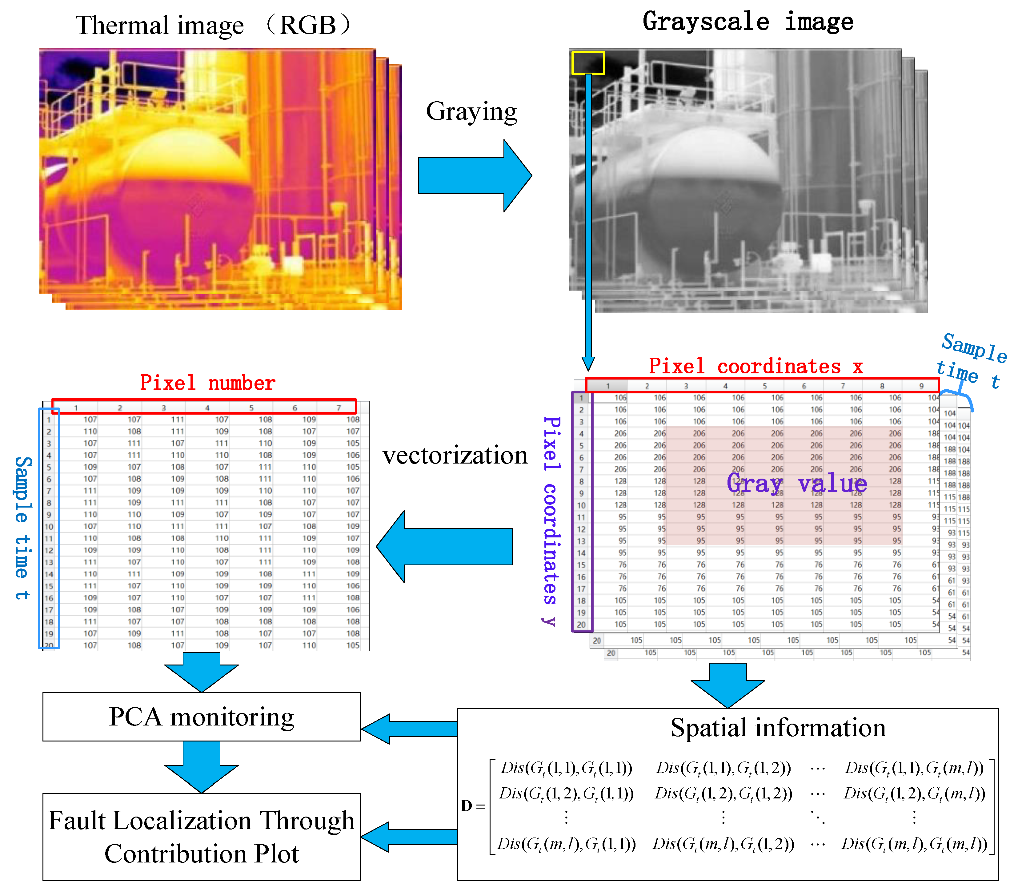
Figure 2 summarizes the procedure presented above.

3.1. Image Data Preprocessing

For the thermal image data set { G t } where G t is the thermal image sample at time t = 1 , 2 , , n , the first step is to convert the 3-channel RGB image to a 1-channel gray image, using the following equation:
G r a y = 0.3 × R + 0.59 × G + 0.11 × B .
where G r a y , R, G , and B are the values in the gray image and the RGB image, correspondingly. As such, the data set { G t } R n × m × l , where m and l are the number of rows and columns in each gray image.
Remark.
Thermal image contains a massive amount of high-dimension data, which introduces a large amount of computation. As such, methods such as Gaussian pyramid [26] can be adopted for image compression.

3.2. Spatial Information-Based PCA (SIPCA)

Before applying PCA, the data set { G t } should be converted into a 2-D matrix first, which means each gray image data G t should be converted into a vector. It should be noted that the thermal distribution is closely related to the spatial distribution, i.e., the pixels with closer spatial distance have a closer thermal relationship. However, spatial information is usually missing when a 2-D matrix gray image is converted into a 1-D vector during the traditional column- or row-expansion operation.
As such, this paper proposes a spatial information-based PCA (SIPCA) method for monitoring thermal image data. First, we construct the following function for measuring the distance between two pixels G t ( i 1 , j 1 ) and G t ( i 2 , j 2 ) as
D i s ( G t ( i 1 , j 1 ) , G t ( i 2 , j 2 ) ) = e ( i 1 i 2 ) 2 + ( j 1 j 2 ) 2 σ ,
where σ is a weight factor with a positive value (e.g., 1). Then convert G t into a 1-D vector, e.g., row-expansion as follows:
X ( t ) = [ G t ( 1 , 1 ) , , G t ( 1 , l ) , , G t ( m , 1 ) , , G t ( m , l ) ] .
Synchronously, the distance matrix is calculated as:
D = [ D i s ( G t ( 1 , 1 ) , G t ( 1 , 1 ) ) D i s ( G t ( 1 , 1 ) , G t ( 1 , 2 ) ) D i s ( G t ( 1 , 1 ) , G t ( m , l ) ) D i s ( G t ( 1 , 2 ) , G t ( 1 , 1 ) ) D i s ( G t ( 1 , 2 ) , G t ( 1 , 2 ) ) D i s ( G t ( 1 , 2 ) , G t ( m , l ) ) D i s ( G t ( m , l ) , G t ( 1 , 1 ) ) D i s ( G t ( m , l ) , G t ( 1 , 2 ) ) D i s ( G t ( m , l ) , G t ( m , l ) ) ]
Therefore, the new covariance matrix S is calculated as follows:
S = 1 n 1 X T D 1 X .
Then, the new PCA model can be obtained by SVD to S . As such, the new PCA method pays more attention to the thermal relationships of adjacent pixels.

3.3. Spatial Information-Based Fault Localization Strategy

However, the contribution plot method can pick out pixels with a high contribution to the fault. However, the high contribution is not equivalent to the high faulty probability, so some normal pixels may be misdiagnosed as fault sources and some faulty pixels may be diagnosed as normal.
When a thermal fault occurs, the pixels in a specific area are abnormal. As such, the following fault localization strategy is proposed.
Step 1. Transfer the contribution score vector to a matrix according to the spatial position of each pixel:
S C o n   S P E i , j = C o n   S P E i l + j .
S C o n   T i , j 2 = C o n   T i l + j 2 .
Step 2. Update the contribution scores with the convolution window function as
1 β 2 a = β β b = β β S C o n   S P E i + a , j + b S C o n   S P E i , j .
where β is the size of the convolution window function. Therefore, fault localization is based on the pixels in a specific area rather than a single pixel, avoiding the wrong fault localization problem.

4. Experiment Test

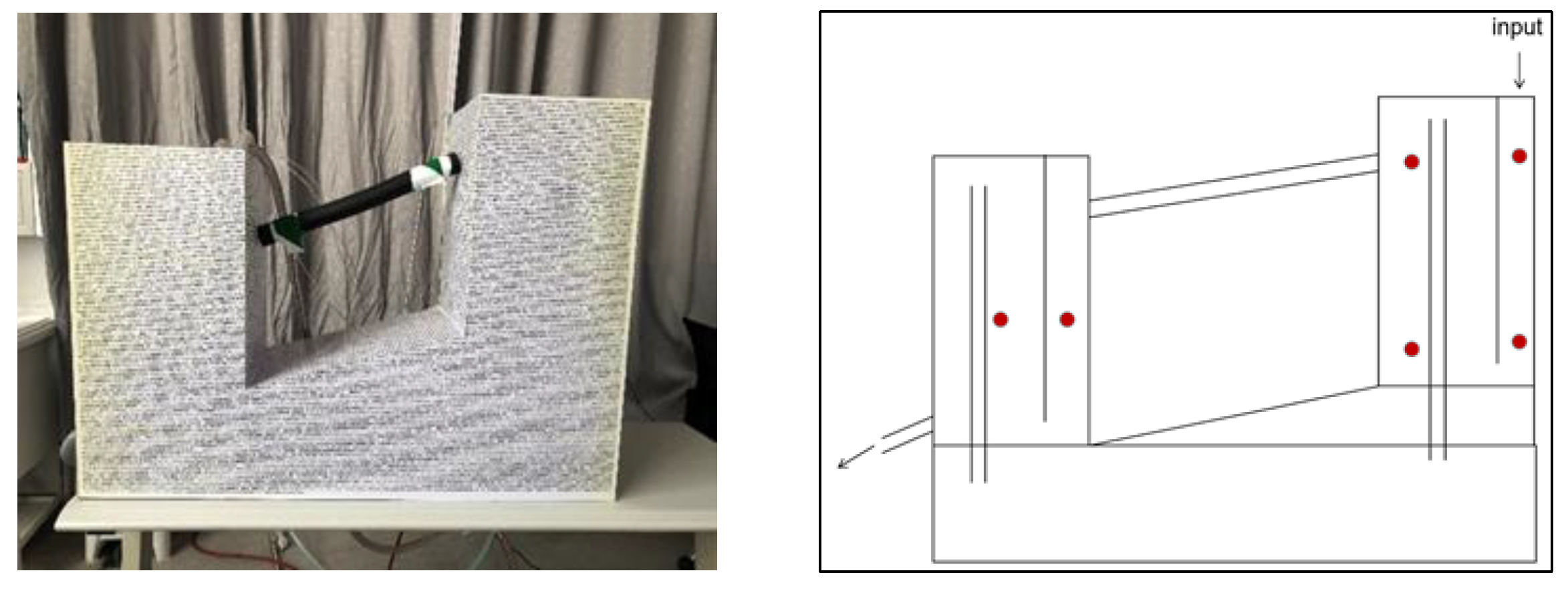
An experimental tank system, shown in Figure 3, is used to test the proposed method, which consists of 2 main tanks. The water inlet of the system is located in the right tank and the outlet is located in the left tank. Two tanks are linked by a tube that is fully insulated, and water flows from the right tank to the left tank. Both tanks have a bulkhead to divide the water tank into two chambers and two chambers connected through the bottom channel. In this experiment, the following equipment are used: thermal camera for obtaining the thermal image (Guide sensmartMobIR air produced by Guide sensmart in Wuhan, China, 25 Hz, and 0.06 °C accuracy); a heating module (CHB401 produced by Hualongdianre in China, <0.5% full scale); and a temperature detection module, which includes 6 temperature sensors (SXPT100 produced by SENSOR in China, 0.15 °C accuracy).
The normal working conditions of the tank system are as follows:
(a)
The heating module is installed near the water inlet position: (a) once the temperature reaches the set upper value (46 °C), the heater will be turned off immediately; (b) until the detected value drops to the lower limit (44 °C), the heater will be turned on again. Thus, the temperature of the whole system is limited to a certain range. The temperature decreases from the right part to the left part.
(b)
All chambers’ water levels are kept at a certain height, e.g., 80%.
And 2000 samples of normal data are collected for model training. The sampling period is 1 s.
In addition, another 2000 samples of data are generated for testing. Each data set contains 2000 samples, and the fault occurs at the 501st sample point. The faults that occurred are of the following three types:
(a)
Peeling of insulation layer to simulate the heat leakage fault;
(b)
Adding another code water inlet in the right chamber of the right tank to simulate an abnormal stable working condition;
(c)
Adding another additional code water inlet into the left chamber of the left tank to simulate the situation in which one chamber’s condition is changed and the other three chambers’ conditions remain unchanged.
For comparison, 6 temperature sensors are installed in the experimental tank system, whose positions are as marked in Figure 3. The data obtained by temperature sensors are monitored by traditional PCA. For both temperature sensors and infrared thermal imaging technology.
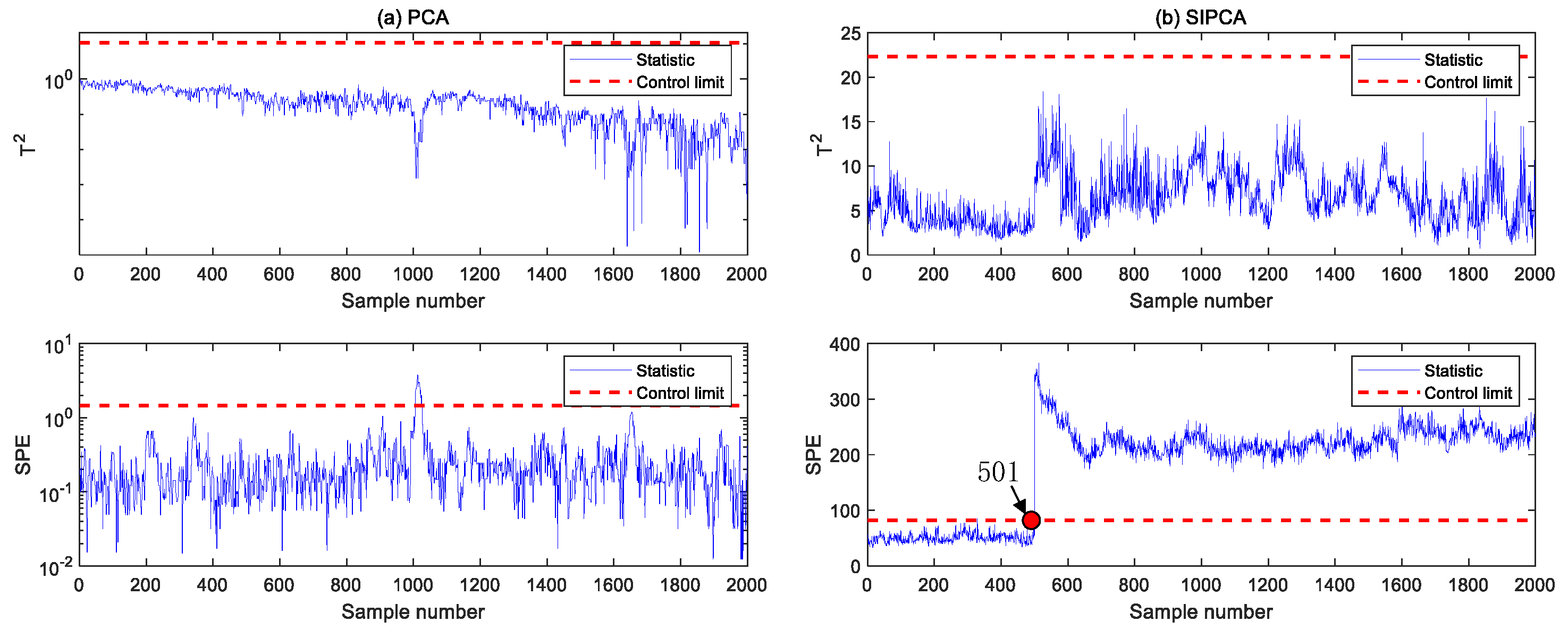
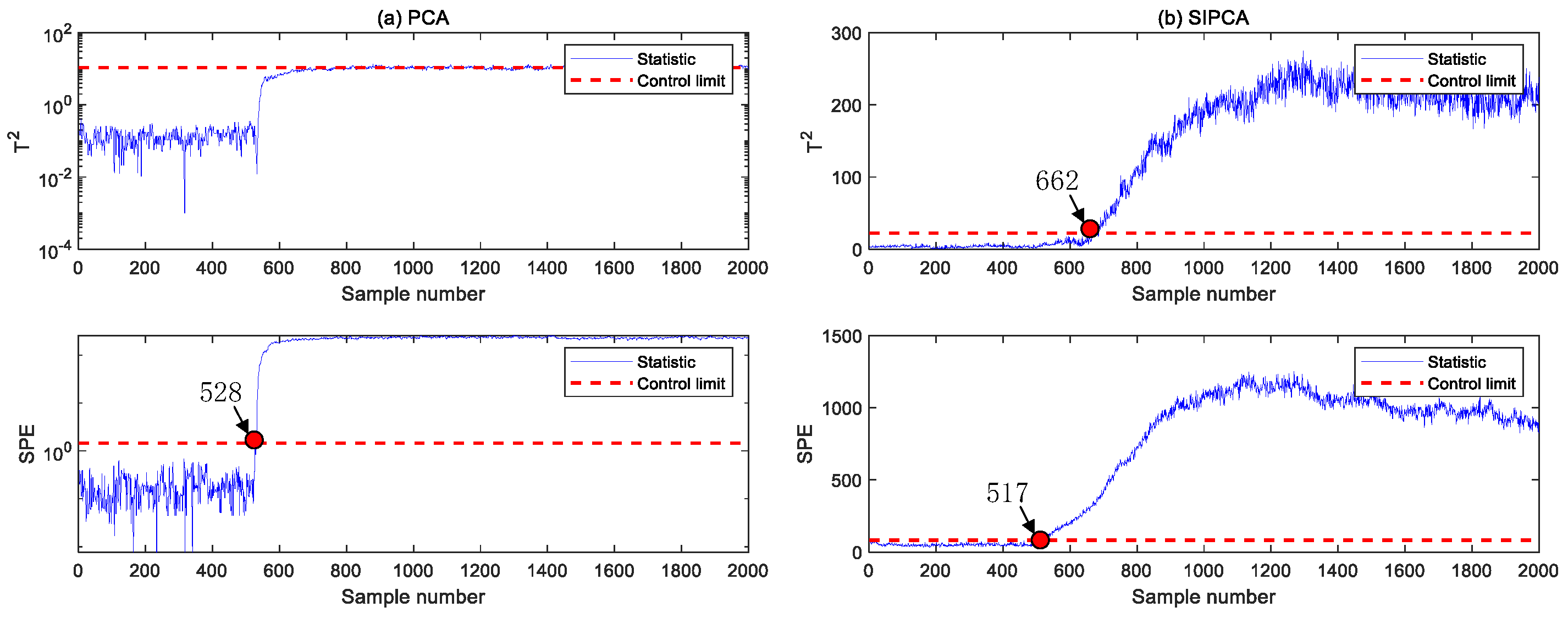
Figure 4, Figure 5 and Figure 6 show the fault detection results of the SIPCA and the traditional PCA approach. As shown in Figure 4, PCA cannot detect Fault 1 because all temperature sensors are only installed in the internal of the experimental tank system and hence PCA cannot detect the temperature anomaly on the surface of the equipment. Different from traditional temperature sensors, a thermal image can successfully catch the temperature change on the object surface, and hence it detects the fault earlier. For both Faults 2–3 in Figure 5 and Figure 6, one gets that SIPCA detects these faults earlier than PCA: SIPCA detects Fault 2 in the 517th sample and PCA detects this fault on the 528th sample; SIPCA detects Fault 3 in the 510th sample and PCA detects this fault on the 558th sample. The reason for this phenomenon is that PCA is based on the data of the temperature sensors, so the detection delay is large when the sensor positions are far from the fault sauce; different from the traditional temperature sensors, the infrared thermal imager monitors the temperature of the process in pixel-level granularity, and hence it can detect this fault earlier. In addition, SIPCA adopts spatial information for model description, so it is sensitive to the temperature variation between adjacent spaces and hence can detect the fault earlier.
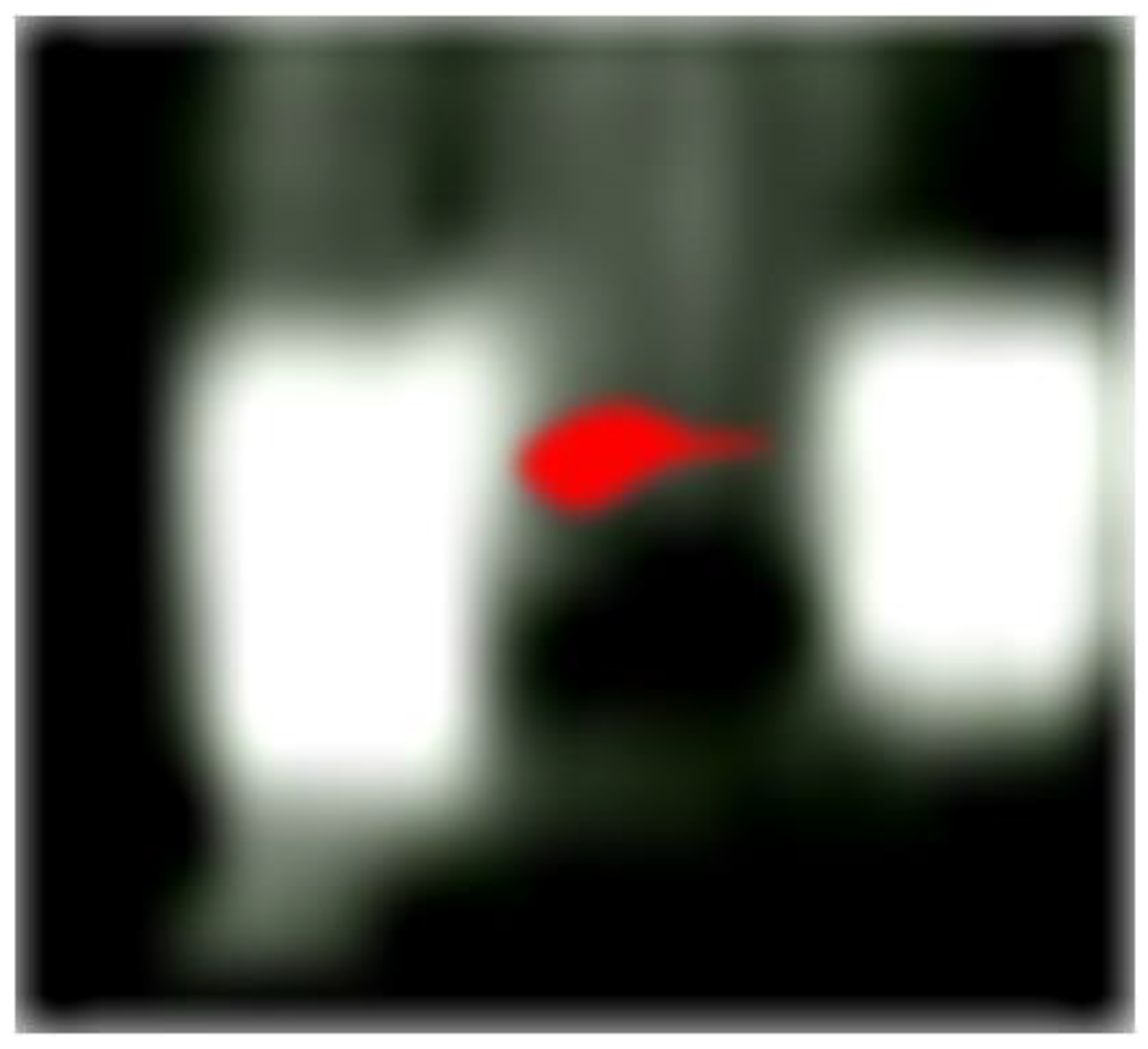
Figure 7 shows SIPCA’s fault localization result for fault 1. Based on the spatial information-based fault localization strategy, SIPCA can successfully locate the fault source position in the image (the red part) and filter out false alarming pixels.

5. Conclusions

In this paper, infrared thermal imaging technology was adopted for measuring the temperature of the equipment/process, and a new PCA called SIPCA was proposed for handling the information in thermal images. SIPCA can introduce spatial information into traditional PCA approaches; hence, it is much more sensitive to temperature variations between adjacent spaces. In addition, spatial information was also adopted in fault localization, and the wrong fault localization problem of the traditional contribution plot method was avoided. Then, the proposed method was tested on an experimental tank system, and the results confirmed that it performs better than the traditional PCA methods.
One drawback of SIPCA is that it is based on a 2D image, and hence it cannot detect the faults that occur on the back of the monitored object. To handle this issue, our future work will focus on the combination of SIPCA with multi-view 3D reconstruction algorithms [27].

Author Contributions

Conceptualization, Z.L. and W.H.; methodology, Z.L.; software, P.S.; validation, P.S., Y.W. and S.L.; formal analysis, Z.L.; investigation, S.D.; resources, S.L.; data curation, W.H.; writing—original draft preparation, Z.L.; writing—review and editing, Y.W.; visualization, S.L.; supervision, S.L.; project administration, S.L.; funding acquisition, S.L. All authors have read and agreed to the published version of the manuscript.

Funding

This research was funded by the Natural Science Foundation of Guangdong Province, China (NO. 2022A1515011040), the Natural Science Foundation of Shenzhen, China (NO. 20220813001358001), and the Young Talents by the Department of Education of Guangdong Province, China (2021KQNCX210).

Institutional Review Board Statement

Not applicable.

Informed Consent Statement

Not applicable.

Data Availability Statement

The data that support the findings of this study are available from the corresponding author upon reasonable request.

Conflicts of Interest

The authors declare no conflict of interest.

References

  1. Venkatasubramanian, V.; Rengaswamy, R.; Yin, K.; Kavuri, S.N. A review of process fault detection and diagnosis: Part I: Quantitative model-based methods. Comput. Chem. Eng. Res. Des. 2003, 27, 293–311. [Google Scholar] [CrossRef]
  2. Li, Z.; Wang, Y.; Hou, W.; Lu, S.; Xue, Y.; Deprizon, S. Neural Component Analysis for Key Performance Indicator Monitoring. ACS Omega 2022, 7, 37248–37255. [Google Scholar] [CrossRef] [PubMed]
  3. Viswanathan, R.; Ramesh, S.; Maniraj, S.; Subburam, V. Measurement and multi-response optimization of turning parameters for magnesium alloy using hybrid combination of Taguchi-GRA-PCA technique. Measurement 2020, 159, 107800. [Google Scholar] [CrossRef]
  4. Tong, C.; Yan, X. Engineering, A novel decentralized process monitoring scheme using a modified multiblock PCA algorithm. IEEE Trans. Autom. Sci. 2015, 14, 1129–1138. [Google Scholar] [CrossRef]
  5. Zhou, P.; Zhang, R.; Xie, J.; Liu, J.; Wang, H.; Chai, T. Data-driven monitoring and diagnosing of abnormal furnace conditions in blast furnace ironmaking: An integrated PCA-ICA method. IEEE Trans. Ind. Electron. 2020, 68, 622–631. [Google Scholar] [CrossRef]
  6. Xu, Y.; Shen, S.-Q.; He, Y.-L.; Zhu, Q.-X. A novel hybrid method integrating ICA-PCA with relevant vector machine for multivariate process monitoring. IEEE Trans. Control Syst. Technol. 2018, 27, 1780–1787. [Google Scholar] [CrossRef]
  7. Lou, Z.; Wang, Y.; Lu, S.; Sun, P. Process Monitoring Using a Novel Robust PCA Scheme. Ind. Eng. Chem. Res. 2021, 60, 4397–4404. [Google Scholar] [CrossRef]
  8. Jiang, Q.; Yan, X. Just-in-time reorganized PCA integrated with SVDD for chemical process monitoring. AICHE J. 2014, 60, 949–965. [Google Scholar] [CrossRef]
  9. Fang, H.; Tao, W.; Lu, S.; Lou, Z.; Wang, Y.; Xue, Y. Nonlinear Dynamic Process Monitoring Based on Two-Step Dynamic Local Kernel Principal Component Analysis. Processes 2022, 10, 925. [Google Scholar] [CrossRef]
  10. AlGhazzawi, A.; Lennox, B. Monitoring a complex refining process using multivariate statistics. Control Eng. Pract. 2008, 16, 294–307. [Google Scholar] [CrossRef]
  11. Bakdi, A.; Kouadri, A.; Bensmail, A. Fault detection and diagnosis in a cement rotary kiln using PCA with EWMA-based adaptive threshold monitoring scheme. Control Eng. Pract. 2017, 66, 64–75. [Google Scholar] [CrossRef]
  12. Kourti, T. Application of latent variable methods to process control and multivariate statistical process control in industry. Int. J. Adapt. Control Signal Process. 2005, 19, 213–246. [Google Scholar] [CrossRef]
  13. Conlin, A.; Martin, E.; Morris, A. Confidence limits for contribution plots. J. Chemom. 2000, 14, 725–736. [Google Scholar] [CrossRef]
  14. Wu, L.; Gang, C. Soft Sensor Method of Temperature Measurement Using CCD Image Color Based on LS-SVM. Energy Procedia 2011, 13, 2229–2235. [Google Scholar]
  15. Yan, W.; Li, K.; Huang, X.; Yu, L.; Lou, C.; Chen, Y. Online measurement of the flame temperature and emissivity during biomass volatile combustion using spectral thermometry and image thermometry. Energy Fuels 2019, 34, 907–919. [Google Scholar] [CrossRef]
  16. Wu, M.; Lei, Q.; Cao, W.; She, J. Integrated soft sensing of coke-oven temperature. Control Eng. Pract. 2011, 19, 1116–1125. [Google Scholar] [CrossRef]
  17. Singh, R.; Sasikumar, T.; Suresh, S.; Ramanan, G. A Novel Detection of Defects in Al–SiC Composite by Active Pulsed Infrared Thermography Using Data and Image Processing. Trans. Indian Inst. Met. 2020, 73, 2767–2783. [Google Scholar] [CrossRef]
  18. Feng, R.Y.; Wang, W.X.; Yan, Z.F.; Wang, D.H.; Wan, S.P.; Shi, N. Fatigue limit assessment of a 6061 aluminum alloy based on infrared thermography and steady ratcheting effect. Int. J. Miner. Metall. Mater. 2020, 27, 139–146. [Google Scholar] [CrossRef]
  19. Glowacz, A.; Glowacz, Z. Diagnosis of the three-phase induction motor using thermal imaging. Infrared Phys. Technol. 2017, 81, 7–16. [Google Scholar] [CrossRef]
  20. Huang, S.L.; Li, C.P.; Chang, C.C.; Tseng, C.C.; Wang, M.W.; Chen, M.L. Real-Time Monitoring of the Thermal Effect for the Redox Flow Battery by an Infrared Thermal Imaging Technology. Energies 2020, 13, 6717. [Google Scholar] [CrossRef]
  21. Janssens, O.; Schulz, R.; Slavkovikj, V.; Stockman, K.; Loccufier, M.; Walle, R.V.D.; Hoecke, S.V.J.I.P. Thermal image based fault diagnosis for rotating machinery. Infrared Phys. Technol. 2015, 73, 78–87. [Google Scholar] [CrossRef]
  22. Wall, M.E.; Rechtsteiner, A.; Rocha, L.M. Singular value decomposition and principal component analysis. In A Practical Approach to Microarray Data Analysis; Springer: Berlin/Heidelberg, Germany, 2003; pp. 91–109. [Google Scholar]
  23. Lou, Z.; Shen, D.; Wang, Y. Preliminary-summation-based principal component analysis for non-Gaussian processes. Chemom. Intell. Lab. Syst. 2015, 146, 270. [Google Scholar] [CrossRef]
  24. Zhang, Y.; Li, S. Modeling and monitoring of nonlinear multi-mode processes. Control Eng. Pract. 2014, 22, 194–204. [Google Scholar] [CrossRef]
  25. Botev, Z.I.; Grotowski, J.F.; Kroese, D.P. Kernel density estimation via diffusion. Ann. Stat. 2010, 38, 2916–2957. [Google Scholar] [CrossRef] [Green Version]
  26. Li, S.; Hao, Q.; Kang, X.; Benediktsson, J.A. Gaussian pyramid based multiscale feature fusion for hyperspectral image classification. IEEE J. Sel. Top. Appl. Earth Obs. Remote Sens. 2018, 11, 3312–3324. [Google Scholar] [CrossRef]
  27. Hu, Z.; Hou, Y.; Tao, P.; Shan, J. IMGTR: Image-triangle based multi-view 3D reconstruction for urban scenes. ISPRS J. Photogramm. Remote Sens. 2021, 181, 191–204. [Google Scholar] [CrossRef]
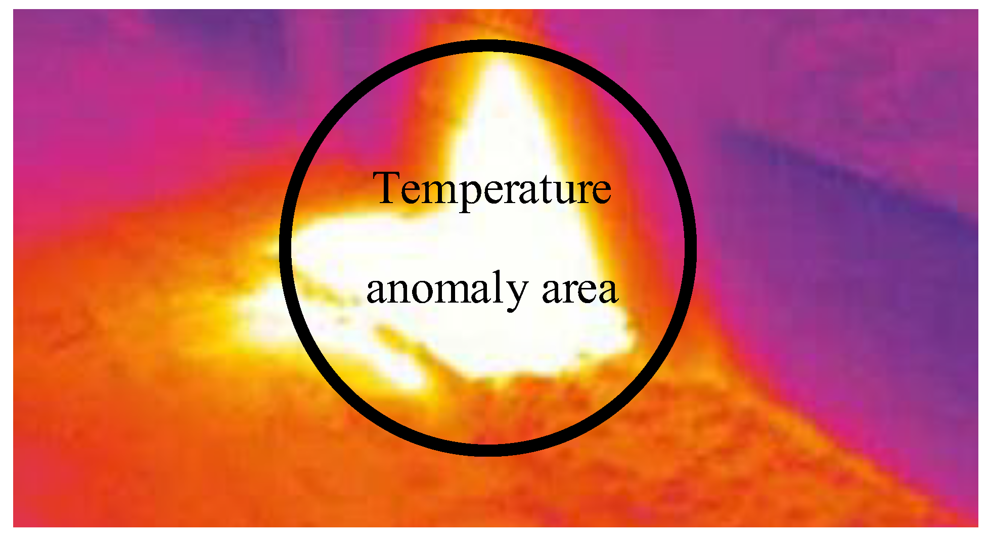
Figure 1. Temperature monitored by infrared thermal imaging.
Processes 11 00589 g001
Figure 2. The proposed method.
Processes 11 00589 g002
Figure 3. Simulated industrial tank. (Red dots are the location of 6 temperature sensors).
Processes 11 00589 g003
Figure 4. Monitoring charts of Fault 1.
Processes 11 00589 g004
Figure 5. Monitoring charts of Fault 2.
Processes 11 00589 g005
Figure 6. Monitoring charts of Fault 3.
Processes 11 00589 g006
Figure 7. Fault localization for Fault 1 (the red part).
Processes 11 00589 g007
Disclaimer/Publisher’s Note: The statements, opinions and data contained in all publications are solely those of the individual author(s) and contributor(s) and not of MDPI and/or the editor(s). MDPI and/or the editor(s) disclaim responsibility for any injury to people or property resulting from any ideas, methods, instructions or products referred to in the content.